Three-dimensional simulation of quenching process of plain carbon steel gears incorporating phase transformations

Abstract

In the present work, a numerical model was developed for the simulation of the quenching process of plain carbon steel gears in water and oil using finite element method. For diffusional transformations, the Johnson–Mehl–Avrami equation was coupled with the additivity rule, while for non-diffusional transformation, the empirical model of Koistinen–Marburger was employed. In addition, the model of Maynier et al. was used to compute the hardness distribution throughout the parts. To evaluate the cooling power of quenching media, the heat transfer coefficients of quenching media were calculated by solving an inverse problem using a stainless steel probe. In addition, a novel approach was applied for computing the actual phase fractions in the multiphase steel. The effects of the latent heat releases during phase transformations along with the effect of temperature and phase fractions on the variation of thermophysical properties were considered. Experimental tests including cooling curve analysis, metallographic investigations and hardness measurements were performed to evaluate the validity of the model. The comparisons indicated that the simulation results were consistent with the experimental results. The multiphase transformation model presented here is capable to predict the distribution of temperature, microstructures and hardness during continuous cooling of steel.

Keywords

Numerical modelling Quenching Phase transformation Steel

Introduction

Heat treatment is an indispensable step in the manufacture of steel products. By deliberate manipulation of the chemical and metallurgical structures of a component, mechanical properties such as hardness, static and dynamic strength and toughness are selectively controlled. However, apart from the desired effects, the heat treatment process can be accompanied by unwanted effects, such as high material hardness, low material strength, a lack of toughness (which can lead to crack formation) and inadequate hardness depth (which can lead to fatigue failure). Therefore, the success or failure of heat treatment not only affects manufacturing costs but also determines product quality and reliability. Heat treatment must therefore be taken into account during development and design, and it has to be controlled in the manufacturing process. For this reason, modelling of heat treatment processes has a great importance to engineers and scientists. Quenching is one of the critical operations in the heat treatment of steel parts, and a large number of researches have been carried out on the mathematical modelling of this process. Many researchers such as Brimacombe et al.,1^–3 Sjöström et al.,4 Denis et al.5^–8and Inoue et al. 9 9,10 have carried out many valuable works on the modelling of phase transformations in steel. However, most of the previous researches have been focused on modelling austenite–pearlite transformation in the eutectoid steel in two dimensions, and less work has been performed on off eutectoid steels in three dimensions. In addition, most of the studies did not consider the diffusionless transformation of austenite to martensite.

Agrawal and Brimacombe1 worked on the modelling of temperature and phase transformation during quenching of eutectoid steel in two dimensions. Wang et al.11 developed a two-dimensional finite element (FE) model for the quenching process of steel cylinders and predicted distributions of temperature and stresses. Kang and Im12carried out the modelling of temperature and phase transformation during the quenching of eutectoid steel in three dimensions. Moreover, Lee and Lee13 have studied the quench distortion in a low alloy steel incorporating transformation kinetics. Recently, Şimşir and Gür14 have investigated the effect of asymmetric geometry on residual stress distribution during quenching of steel.

In the present study, a coupled thermomicrostructural numerical model was developed to simulate thermal history and phase transformations during the continuous cooling of a plain carbon steel. It was attempted to minimise the idealistic assumptions. Thus, the applied thermophysical properties of steel were assumed to be functions of both temperature and volume fraction of various phases. In addition, the latent heat releases during phase transformations were considered in the computations. The developed model was employed to simulate the quenching process of plain carbon steel gears in water and oil. In order to increase accuracy of the model, a stainless steel probe was used to evaluate the cooling power of the quenching media. Then, using an inverse solving technique, the heat transfer coefficients of the media were calculated. All types of phase transformations, i.e. ferritic, pearlitic, bainitic and martensitic, are probable to occur in the steel under study. Therefore, a multiphase transformation model was developed to calculate the maximum attainable and final volume fraction of each phase. To evaluate the reliability of the model, the thermal history of the specimens was recorded, and metallographic and hardness analyses were performed on the specimens.

Numerical model

The models involved in the present numerical procedure can be divided into three categories: heat transfer model, phase transformation model and hardness model.

Heat transfer model

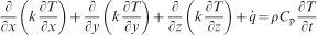
The transient heat conduction equation, including the internal heat source, can be described as15 (1) where T and t are the temperature and the time respectively, ρ, C_p and k are the density, the specific heat and the thermal conductivity respectively, and is the rate of the latent heat releases due to phase transformation.

The thermophysical properties of steel are functions of two parameters: temperature and volume fraction of various phases. They are calculated according to the rule of mixtures as below (2) where , and are the thermal conductivity, the specific heat and the volume fraction of the ith phase at the jth time step respectively.

During the continuous cooling of steels, due to the phase transformations, latent heat releases. In order to increase the accuracy of the simulation, this effect was considered in the model. The amount of heat releases during phase transformation can be calculated as (3) where ΔH_i is the amount of heat releases at temperature T_i, and ΔX_i is the amount of phase transformation during the time step Δt.

The initial condition for this problem is the initial temperature of the specimen. The austenitising temperature of steel T₀ was assumed as the uniform initial temperature of the specimen (4) The boundary condition of this problem can be described as (5) where n is the outer normal of the surface boundary, h is the convective heat transfer coefficient, T_S is the surface temperature and T_A is the ambient temperature.

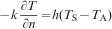
The numerical simulation of metallurgical transformations occurring during continuous cooling requires accurate heat transfer conditions at the boundaries of the specimens. In the present study, a cylindrical probe of AISI 304 stainless steel with 12·5 mm diameter and 60 mm length was used to obtain the convective heat transfer coefficient during quenching. AISI 304 stainless steel was selected because no latent heat is generated by phase transformation during its heat treatment. A K type thermocouple was embedded in the probe to record the thermal history of a point near its surface. This probe was heated up and then quenched in the quenching medium. The published thermal properties of AISI 304 stainless steel16and the measured surface temperatures were employed to compute the heat transfer coefficient. Finally, the convection heat transfer coefficient was calculated as a function of temperature by an inverse algorithm. The resultant heat transfer coefficients for quenching in still water and still oil, under the experimental conditions of the present work, are shown in Fig. 1.

Figure 1

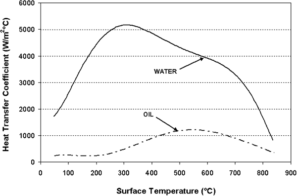
Heat transfer coefficient as function of temperature for quenching in still water and still oil

Phase transformation model

The phase transformations in steel consisted of diffusional and non-diffusional phase transformations. The governing equations for each type of these transformations are as follows.

Diffusional phase transformations

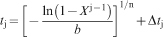
There are many kinetic equations for the description of diffusional transformations. One of the most famous equations is the Johnson–Mehl–Avrami (JMA) equation.17^–19 According to this equation, the progress of phase transformation in a constant temperature can be computed as a function of time (6) where is the volume fraction of the ith phase in the jth time step, and b and n are the material parameters that for each grade of steel can obtained from the TTT diagram using the following equations (7) (8) where t_s and t_f are the start and termination times of the phase transformation at a certain temperature. X_s and X_f are the relevant volume fractions of the phase transformation and are usually assumed to be 0·01 and 0·99 respectively.

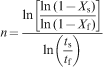
However, the JMA equation cannot be used in non-isothermal conditions. Thus, the additivity rule20 was applied to simulate continuous cooling condition. According to this rule, the cooling curve was divided into a number of small time steps, and the amount of transformation in each time step was calculated using the JMA equation. The time elapsed from the beginning of the transformation t_j was calculated as below (9) Regarding the additivity rule, the transformation begins when the following condition is satisfied (10) where Δt_j is the jth time step, and τ_j is the transformation incubation time at temperature T_j.

Non-diffusional phase transformation

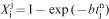
The empirical model of Koistinen and Marburger21was employed to model the kinetics of non-diffusional phase transformation. Using this model, the volume fraction of martensite can be calculated according to the temperature below M_s (11)

Off eutectoid phase transformation model

Since the JMA equation is based on a total fraction of unity, it is necessary to convert the obtained fractions of the JMA equation to the actual fractions. In other words, the transformation data must be normalised. For the formation of proeutectoid ferrite, there is a maximum amount of austenite that can be transformed into ferrite. Many researchers have computed this amount using the lever rule in the hypoeutectoid region of the Fe–Fe₃C phase diagram. However, the isothermal tests for hypoeutectoid steels have shown that the total volume fraction of ferrite decreases with decreasing transformation temperature below Ac₁.13 However, the results of this approach are not consistent with the experimental results. To overcome this problem, some researchers 2 2,22have extrapolated the γ/Fe₃C and α/γ equilibrium phase boundaries of the Fe–Fe₃C phase diagram linearly to the lower temperatures. However, both of these approaches employ the equilibrium phase diagram of Fe–Fe₃C and neglect the effects of alloying elements. This way could not be suitable either, as the equilibrium phase boundaries move by alloying elements, changing the maximum attainable fraction of ferrite. It should be noted here that no theory is still available to define functions for maximum transformable austenite to pearlite and bainite in steels. 22 22,23 For these phases, most of researchers have considered the maximum transformable amount of austenite as unity, while others have estimated these amounts from IT diagrams.

In the present study, a new approach was developed to compute the actual fraction of each phase. In this approach, instead of calculating each phase fraction by the JMA equation and multiplying it by the maximum attainable phase fraction, the amount of austenite decomposition was computed. In fact, in addition to the calculation of the factors b and n for ferrite, pearlite and bainite, these factors were calculated for austenite decomposition. Then, the JMA equation and the additivity rule were employed to compute the amount of austenite decomposition at each time step. In addition, by application of the JMA equation and the additivity rule for the transformations of ferrite, pearlite and bainite, the times of initiation and termination of each phase transformation could be predicted. Figure 2 shows the flowchart of the approach applied for the simulation of phase transformation kinetics. In this chart, X_A, X_F, X_P, X_B and X_M are fractions of austenite, ferrite, pearlite, bainite and martensite respectively, and T_F, T_P and T_B are the maximum temperatures for transformations of austenite to ferrite, pearlite and bainite respectively.

Figure 2

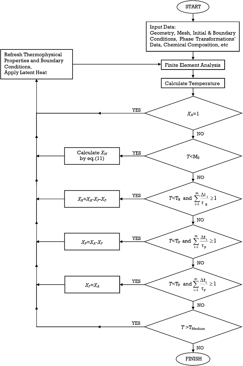
Flowchart of procedure applied for simulation of multiphase transformation kinetics

Hardness model

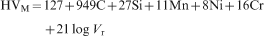
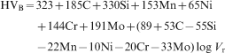
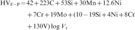
In order to predict the hardness distribution in the quenched parts, the model of Maynier et al.24was employed. In this model, the hardness of each phase can be calculated using chemical composition and cooling rate. The computational model for various phases can be expressed as below (12) (13) (14) where HV_M, HV_B and HV_F-P are the Vickers hardness of martensite, bainite and mixture of ferrite and pearlite respectively. C, Si, Mn, Ni, Cr, Mo and V are the weight per cents of various alloying elements in steel, and V_r is the cooling rate at 700°C (°C h⁻¹).

The total hardness at each element was calculated using the rule of mixtures (15) where HV is the total Vickers hardness of steel, and X_M, X_B, X_F and X_P are the volume fractions of martensite, bainite, ferrite and pearlite respectively.

Materials and experiments

The plain carbon steel considered in the present study was AISI 1045 with the chemical composition of 0.49C–0.24Si–0.79Mn–0.10Ni–0.09Cr–0.08Mo. It is a heat treatable plain carbon steel with relatively good workability and machinability. The conventional heat treatment for this steel is quenching followed by tempering, and its major application is in vehicular industries. As can be seen in the continuous cooling transformation diagram of AISI 1045 (Fig. 3), all types of transformations, i.e. ferritic, pearlitic, bainitic and martensitic, are probable in this steel.

Figure 3

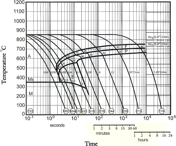
Continuous cooling transformation diagram of AISI 1045 steel25

To improve the accuracy of the simulations, the thermophysical properties were assumed to be functions of temperature and type of microstructure. Figure 4 shows the variation in thermal conductivity and specific heat according to the temperature and the type of microstructure in this steel. 16 16,26 Moreover, a constant value of 7850 kg m⁻³ was considered as the density of this steel. It should be noted that the thermophysical properties of ferrite, pearlite and bainite were supposed to be similar, and the specific heats of martensite and austenite at low temperatures were calculated by extrapolation of those of austenite at high temperatures.

Figure 4

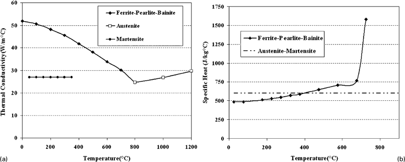
Thermophysical properties of AISI 1045 steel according to temperature and type of microstructure

In order to calculate the latent heat releases during diffusional phase transformations, the published data27were used as equations (16) and (17). In addition, the latent heat (J cm⁻³) of bainitic transformation was assumed to be the same as that of pearlite (16) (17) In the case of martensitic transformation, a constant value proposed by Ericsson et al.28 was applied as the latent heat (J cm⁻³) (18) In the above equations, ΔH_F, ΔH_P-B and ΔH_M are the enthalpy changes due to ferrite, pearlite or bainite and martensite transformations respectively.

The quenching process of AISI 1045 steel gears was simulated to predict the final distribution of microstructures and hardness. Figure 5 illustrates the mechanical draft of the gear studied in the present work.

Figure 5

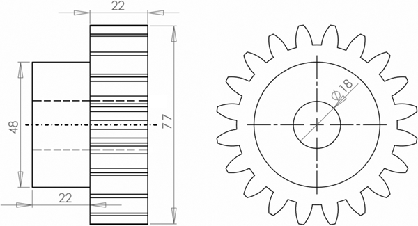
Draft of gear considered in present work: all dimensions are in millimetres

The present simulation was conducted using the commercial FE software ANSYS 10·0, and the model was developed by programming in ANSYS parametric design language capability of the software. Owing to symmetry, only half of a gear tooth was considered in the modelling. Figure 6 depicts the FE mesh used in the simulations. In order to validate the numerical model, the experimental tests were performed on actual steel gears of AISI 1045. The thermal histories of the specimens were measured by K type thermocouples with diameter of 0·3 mm. A personal computer with an integrated PCI-773 measuring card (Eagle Technology) and LabView 5·1 software was used to record the measured thermal cycles. In addition to the cooling curve measurements, the parts were cut after quenching, and metallographic and hardness tests were performed on the specimens.

Figure 6

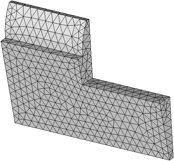
Model and FE mesh used in simulations

Results and discussion

Figure 7 shows the cooling history of the gears quenched in water and oil respectively. Three locations within the gear (A, B and C) were considered for the analysis, among which the thermal history of a point near the surface (A) and a point near the centre of the part (C) was measured experimentally. A good agreement was observed between the recorded cooling curves and the simulated ones, both near the surface and the centre of the specimens, which indicates that the applied boundary conditions, thermophysical properties and heat generations due to phase transformations were appropriately consistent with actual conditions. It is obvious that the quench severity of water is much more than oil. However, the cooling curves of various points among oil quenching are closer to each other in comparison with the water quenching. This shows that the uniformity during oil quenching is more than water quenching.

Figure 7

Predicted and experimental thermal histories at different points of gears quenched in a water and b oil

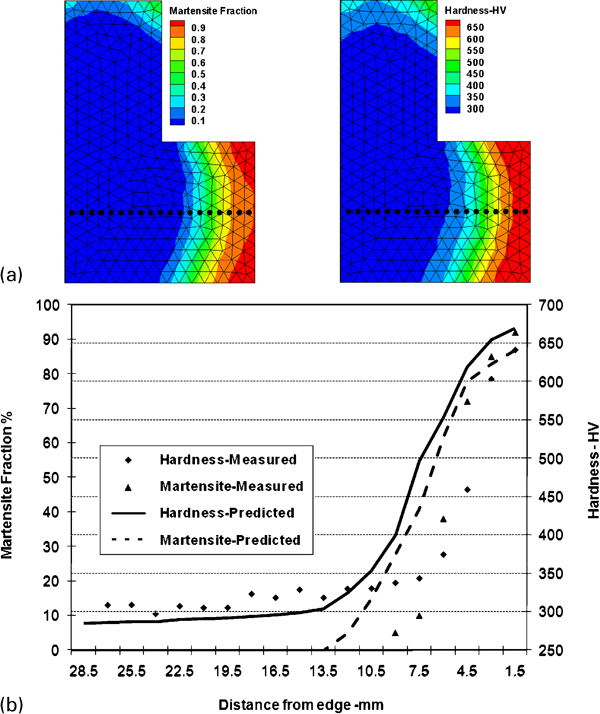
Figure 8 shows the simulated and experimental distributions of martensite and hardness in the water quenched samples. The solid points on the contours indicate the locations in which hardness measurements were made. Similarly, Fig. 9 shows the simulated and measured distributions of martensite and hardness in the oil quenched parts. In the water quenched specimen, due to the high quench severity of water, more than 90 of austenite is transformed to martensite, even at the centre of the gear. Hence, the hardness is high throughout the gear. On the other hand, in the oil quenched gear due to the low quench severity of oil and the low hardenability of the AISI 1045 steel, martensitic transformation occurred only at the edges, while at the gear teeth and the inner points, most of the austenite is transformed to ferrite and pearlite. Thus, a higher hardness at the teeth and a lower harness at the central regions are achieved.

Figure 8

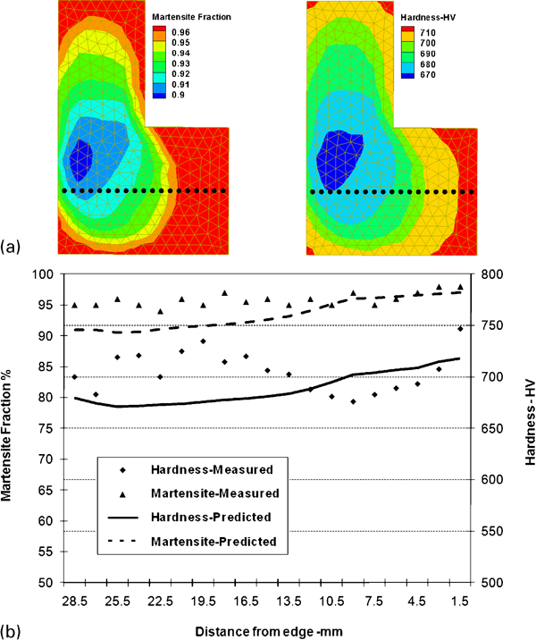
Comparison between predicted and measured distributions of hardness and martensite in gear quenched in water

Figure 9

Comparison between predicted and measured distributions of hardness and martensite in gear quenched in oil

As can be seen, there is a good consistency between the simulated and experimental results. The inconsistencies observed in some results might have several sources. Some errors may come from the experimental procedures such as metallography and chemical analysis (hardness predictions). Another source of error might be due to dissimilarities of the chemical composition and the primary austenite grain size of the specimens compared to those of samples used for the development of TTT diagrams.

Figure 10 shows the simulated distribution of ferrite, pearlite, bainite and martensite all over the gears quenched in water and oil. As mentioned previously, because of the high cooling power of water, martensite is the predominant phase throughout the specimen, and the amount of diffusional phases is small.

Figure 10

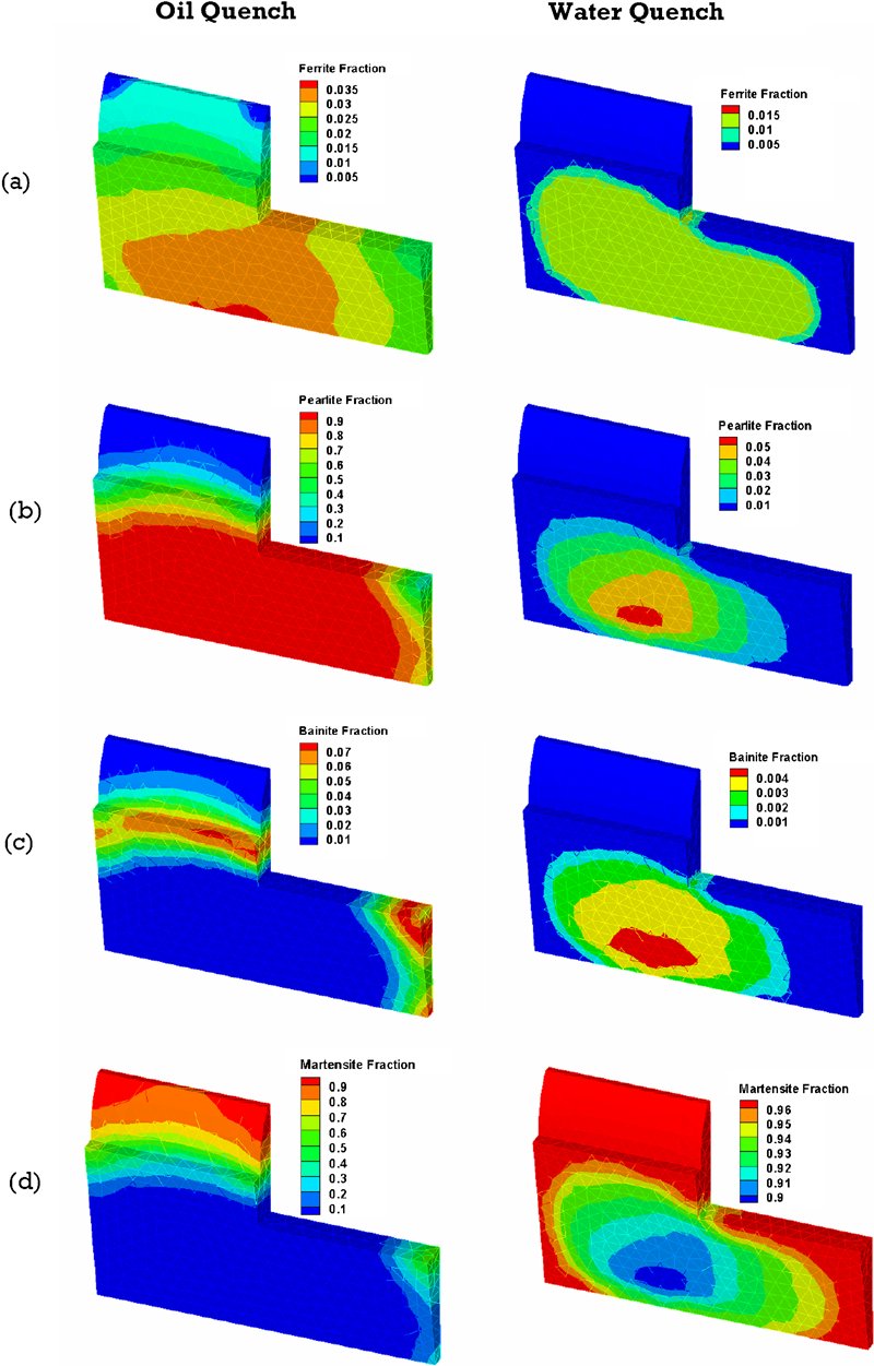
Simulated distribution of a ferrite, b pearlite, c bainite and d martensite in gear quenched in oil and water

However, in the oil quenched gear, because of the low cooling power of oil, the predominant phase is pearlite, and martensite only exists at the edges and the teeth, where due to the thinness of the sections, the cooling rate is relatively high.

The place in which the maximum amount of bainite appears is also noteworthy. It should be noted that AISI 1045 is not a bainitic steel, but bainite transformation can only occur under certain cooling conditions. The transformation of austenite to bainite occurs in moderate cooling rates. At points with high cooling rates, most of the austenite is transformed to martensite. On the other hand, at slow cooling rates, the amount of austenite which is decomposed to ferrite and pearlite increases, and thus, there is less retained austenite available for bainite transformation. However, due to the different quench severities of water and oil, the place in which this moderate cooling rate happens and the maximum amount of bainite appears is different in water and oil quenching.

Conclusions

In the present work, a 3D numerical model was developed to simulate the quenching process of a plain carbon steel in water and oil. It was found that most of the austenite throughout the gear was transformed to martensite during quenching in water. Therefore, the gear completely hardened. However, the results showed that the oil could not provide sufficient cooling rates for hardening a plain carbon steel like AISI 1045, and the hardening happened only at the edges and thin sections. Therefore, regarding the low hardenability of this steel, oil quenching was not suitable for hardening this steel.

Comparing the simulation and experimental results, it can be concluded that the developed model is appropriately able to simulate various types of phase transformations and to predict the final distribution of microstructures and hardness in quenched parts. The model can be employed as a design tool to achieve the optimised process conditions in industrial applications.

References

Agrawal

, Brimacombe

: Metall. Trans. B , 1981, 12B, 121–133.

Howbolt

, Chau

, Brimacombe

: Metall. Mater. Trans. A , 1985, 16A, 565–578.

Kamat

, Hawbolt

, Brown

, Brimacombe

: Metall. Trans. A , 1992, 23A, 2469–2690.

Sjöström

: Mater. Sci. Technol. , 1985, 1, 823–829.

Denis

, Gautier

, Simon

AGB

: Mater. Sci. Technol. , 1985, 1, 805–814.

Denis

, Gautier

, Sjöström

: Acta Metall. , 1987, 35, 1621–1632.

Denis

, Sjöström

, Simon

: Metall. Trans. A , 1987, 18A, 1203–1212.

Denis

: J. Phys. , 1996, 6, 159–174.

Inoue

, Wang

: Mater. Sci. Technol. , 1985, 1, 845–850.

10.

Inoue

, Ju

, Arimoto

: Proc. 1st Int. Conf. on ‘Quenching anddistortion control’, (ed. , Totten

G E

, ed), 205–212; 1992, Chicago,IL, ASM International.

11.

Wang

, Chandrasekar

, Yang

HTY

: Trans. ASME J. Eng. Ind. , 1993, 115, 124–138.

12.

Kang

, Im

: J. Mater. Process. Technol. , 2007, 183, 241–248.

13.

Lee

, Lee

: Acta Mater. , 2008, 56, 1482–1490.

14.

Şimşir

, Gür

: J. Mater. Process. Technol. , 2008, 207, 211–221.

15.

Holman

: ‘Heat transfer’, 67; 1976, NewYork, McGraw-Hill.

16.

Bagdade

: ‘Thermal properties of metals’; 2002, MetalsPark, OH, ASM International.

17.

Johnson

, Mehl

: Trans. AIME. , 1939, 135, 416–458.

18.

Avrami

: J. Chem. Phys. , 1939, 7, 1103–1112.

19.

Avrami

: J. Chem. Phys. , 1940, 8, 212–224.

20.

Scheil

: Arch. Eisenhüttenwes. , 1935, 12, 564–567.

21.

Koistinen

, Marburger

: Acta Metall. , 1959, 7, 59–60.

22.

Reti

, Fried

, Felde

: Comput. Mater. Sci. , 2001, 22, 261–278.

23.

Kirkaldy

, Venugopalan

, McGirr

: Proc. 1st National Conf. on ‘Heat treatment’, Sydney,NSW, Australia, August, 1984, AustralianInst. of Metals, 1–23.

24.

Maynier

, Dollet

, Bastien

: Proc. Int. Conf. AIME, (ed. , Doane

D V

, Kirkaldy

J S

, ed), 518–544; 1978, NewYork, AIME.

25.

‘Theguide for heat treatment of IASC1191 steel’, Technicalreport, Isfahan Alloy Steel Company, Isfahan,Iran, 2007.

26.

Griffiths

: ‘Physical constants of some commercialsteels at elevated temperatures’, 3; 1953, London, Butterworths Scientific Publication.

27.

Darken

, Gury

: ‘Physical chemistry of metals’, 415; 1953, New York, McGraw-Hill.

28.

Ericsson

, Sjöström

, Knuuttila

: Proc. Int. Conf. on ‘Case hardened steels’,(ed. , Diesburg

D E

, ed); 1983, Warrendale, PA, TMS-AIME.