
Abstract
Two dual phase steels with markedly different microstructural banding have been serial sectioned for characterisation and quantification of the banding in three dimension (3D). Two parameters, bounded on a scale of zero to one, have been defined to quantify the amount of microstructural banding in two dimension (2D). The band continuity index Cb quantifies the continuity of each band within the band. The perpendicular continuity index Cp describes the continuity between adjacent bands. In the present work, these parameters are extended and applied to full 3D bands. The results show that while the connectivity of bands in 3D is different than what is observed in 2D, the quantification of banding with these parameters in 2D is sufficient to accurately represent the banding in 3D, thus validating these newly defined parameters.
Introduction
Microstructural banding is an important phenomenon in steel manufacturing. Bands in a material can cause the mechanical properties to be anisotropic.1 Anisotropy can be useful in certain applications where strength is desired in one direction and flexibility in the other. On the other hand, it can cause serious problems in working with the material, for example, when machining it. Until now, banding has only been studied and quantified using two-dimensional (2D) images under the assumption that the observations extend to three dimension (3D) without actual validation.2–7 While it is well known that for random structures this assumption holds,8,9 it has not yet been demonstrated for materials with high degrees of correlation, such as banded materials. One of the aims of the present work is to carefully analyse the banding behaviour of two distinctly different microstructures using serial sectioning to observe in 3D.
The companion paper to the present work7 defines two new parameters that quantify the degree of banding in 2D microstructures, which are bounded on the interval [0,1] and calculated from standard material values. These parameters can be found from any microscopy or diffraction method that distinguishes between phases in the microstructure. The first parameter is called the band continuity index Cb, and it describes the strength of banding along the direction of the bands. It is calculated for each band, and the average over the bands is taken to represent the structure as a whole. The second parameter is called the perpendicular continuity index Cp, and it describes the strength of banding with respect to the distribution of the bands throughout the material. Another aim of the present work is to extend the parameters from 2D to 3D and validate that the 2D quantification is sufficient to represent what can be seen in 3D.
Background
There are a variety of means to observe the surface of prepared materials. Optical microscopy, electron microscopy (SEM, TEM, scanning transmission electron microscopy, etc.), diffraction [X-ray diffraction (XRD), electron backscatter diffraction (EBSD), etc.] and energy dispersive spectroscopy all provide various types of information about a material at various resolutions. Microscopy provides spatial information about the microstructure. Often, the grain boundaries and solute particles are directly observable with the right etching agent. Diffraction can provide information on the crystallographic orientations and textures of the microstructures. When these two methods are used in conjunction, much of the microstructure is sufficiently characterised. However, most of this information is limited to the observable 2D surface. Through stereology, some information observed from the image can be extrapolated into 3D.9 Much of this information is limited to averages; individual details are often not extractable. For example, it is not possible to obtain information about the connectivity, contiguity or real particle shape and size in the depth of the material by only observing a 2D image.10–13 Obtaining full 3D information about a material is important for a full understanding of the mechanical properties of the material.10–14
There are currently two ways to experimentally obtain the 3D information: serial sectioning combined with one of the above microscopy methods11–13,15–17 and X-ray tomography and diffraction.18,19 Serial sectioning is perhaps the oldest technique and has the advantage of being relatively simple since it can be accomplished with polishing equipment and an optical or electron microscope.10,11,13,15–17 With microscopes, multiple spatial resolutions can be obtained in a single imaging step, and orientation information can be obtained from EBSD. Often, the limiting factor with serial sectioning is the amount of material that can be removed with each polishing step. The removal depth must be a small fraction of the grain size in order to retain useful information about the microstructure, and even then, some information is lost.10 This becomes time consuming since a large number of images are required to represent a significant depth into the material, and often, the polishing, etching and imaging must be done in separate locations. This leads to difficulties in aligning and registering the images.11,12,16,17 Automation of serial sectioning is of interest,11 and recently, focused ion beam etching has been used both to remove significantly thinner layers for increased depth resolution and to automatically remove a layer while simultaneously imaging the microstructure with SEM or EBSD.12,16 The biggest drawback of serial sectioning is that it is destructive and, therefore, it cannot be used to observe the temporal behaviour of the microstructure.17–19
In comparison, X-ray tomography and 3D XRD are non-destructive to the sample.18–20 Powerful enough X-rays can penetrate hundreds of micrometres into the material with resolution down to the nanometre scale18 and can obtain orientation information about the individual grains in the sample. Another advantage of XRD over serial sectioning is the ability to observe the in situ development of the microstructure during annealing or recrystallisation.19,20 The drawback of this technique is the cost of creating X-rays; synchotron sources are required for penetrating deep enough into the material and providing high enough resolution.18,19
Another means of obtaining 3D information is through simulation and modelling. Several simulation techniques, such as finite element methods, cellular automata and Voronoi methods, are used to create realistic microstructures and then to evolve those microstructures by means of established physical models for describing the behaviour of the microstructures under certain conditions. Currently, serial sectioned data or images taken from the three orthogonal planes of a material are used as input into simulations to obtain the most realistic microstructures possible.16,18 The distinct advantage of simulations is that they are extremely cost effective. Using models and simulations allows for 3D observations of the microstructures during events such as grain nucleation and recrystallisation that are not easily accessible with experiments due to equipment, time and/or resource constraints. Most models make assumptions, and often, these assumptions are made to simplify the problem. However, the assumptions may not actually hold in real microstructures, and as more 3D data are being obtained, the model assumptions need to be reconsidered.10,16,19,20
Experimental
Data acquisition
In the present work, two DP800 steels having the same chemical composition (Table 1) but different rolling conditions were serial sectioned for comparison. The two steels were chosen because of the stark visual differences in the banding of the microstructures, with steel B appearing more banded than steel A.
Composition of DP800 steels
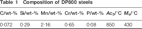
Initially, the samples were prepared in a typical manner for optical microscopy: polishing began with 320 grit wet sandpaper with subsequent processing to finer paper, finishing with 6, 3 and 1 μm polishing cloths and the corresponding diamond suspensions. This was followed by etching in 5 nital, and the samples were examined using a Leica DM-LM microscope with a computer controlled PRIOR Scientific Instruments table. The images were captured with a Leica DFC420C camera, which was controlled by Leica QWin Pro V 3·5·1 (April 2008) software. Images of the planes perpendicular to the rolling (RD), transverse (TD) and normal (ND) directions were taken at six different magnifications: ×500, ×200, ×100, ×50, ×25 and ×12·5. The analysis of the present paper is presented for the plane perpendicular to the RD at the magnification of ×500.
For each subsequent section, a layer was removed by polishing. The first 23 layers were removed with the 1 μm polishing cloth and diamond suspension. Each polishing step removed ∼0·5 μm, as measured and aligned with Vicker's hardness indents just outside the desired field of view. Beginning with step 24, both 3 and 1 μm cloth/diamond suspensions were used. This led to ∼3 μm removal with each step. It was determined that the smaller step size required more time than was available to section into the depth of interest, and so the larger step size was used for the second half of the sectioning.
Figure 1 shows original images as taken from the microscope for steel A. The images shown are of the plane normal along the TD, which is also the direction along which the sectioning occurs. The phases are ferrite (light areas), martensite and retained austenite (dark areas). In the present work, we are primarily interested in characterising, comparing and quantifying the banding of the ferrite phase in the microstructures. While the choice of the banded phase will provide different output values, either phase may be chosen to carry out this analysis.
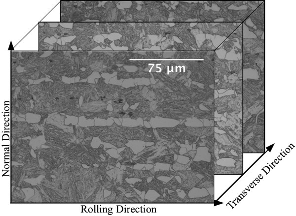
Original image for ND–RD plane of steel A: serial sectioning (atotal of 55 slices) is along TD
Image processing
The initial image processing was performed using the freeware program Fiji21 on the optical images. All section images (heretofore referred to as slices) were put into a TIFF image stack, which was registered and cropped so that the images are properly aligned and rotated. The remaining image processing steps were carried out on the entire stack. First, the stack contrast was enhanced by equalising and normalising the grey scale histogram for all 55 images. Next, the brightness/contrast for the stack was adjusted by hand in order to accentuate the differences between the two phases. This makes the ferrite phase black and the martensite phase white in the binary images. Finally, the image was thresholded to create a binary mask to separate the two phases. All subsequent image processing and data analysis were carried out on these binary images, as described in the companion paper.7 Briefly, the images were filtered to remove small bits of ferrite in the matrix. The images underwent morphological processing to eliminate the grain boundaries within a band because the bands themselves are of more interest than the individual grains. This processing consists of dilating and closing the image with a 3 pixel (0·7 μm) horizontal line.
Threshold banding
From the thresholded, filtered, dilated and closed images, a profile was created by taking the average of the grey scale values in the horizontal direction (RD), which coincides with the banding direction. To determine the ferrite bands, a grey scale threshold is defined so that any value above the threshold is considered to be part of a stylised ferrite band (demarcated as the region between the solid and dashed line pairs), and any value below is considered to be part of the background, as in Fig. 2b. The details of this procedure can be found in the companion paper.7 Moreover, the individual profiles are quite rough, so a spline fit was constructed using an automated fitting routine22 to smooth out the curves. Figure 2a shows the actual profile (crosses) and the spline smoothed fit (solid line) for both steels A and B. Using a smooth profile is important for defining a band because the rougher the profile, the more likely it is for a band to be broken into tiny, disconnected bands by the threshold, and then it is no longer an accurate representation of the banding in the microstructure.
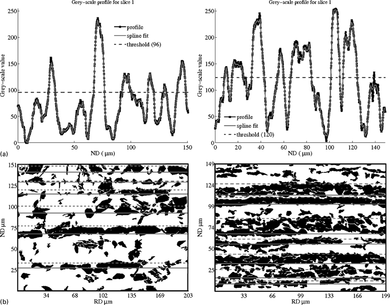
Creating stylised banded structures from profiles (steel A, left; steel B, right)
Results and discussion
Initial 3D microstructure analysis
The first step to characterising the bands in 3D is to look at the profiles, as described in the previous section, for each slice in the stack. These profiles highlight the regions where bands exist before imposing boundaries on them through the thresholding procedure. In Fig. 3a, these profiles are stacked consecutively in the slicing (or transverse) direction. This provides a glimpse of how the ferrite bands behave in the TD or sectioning direction.
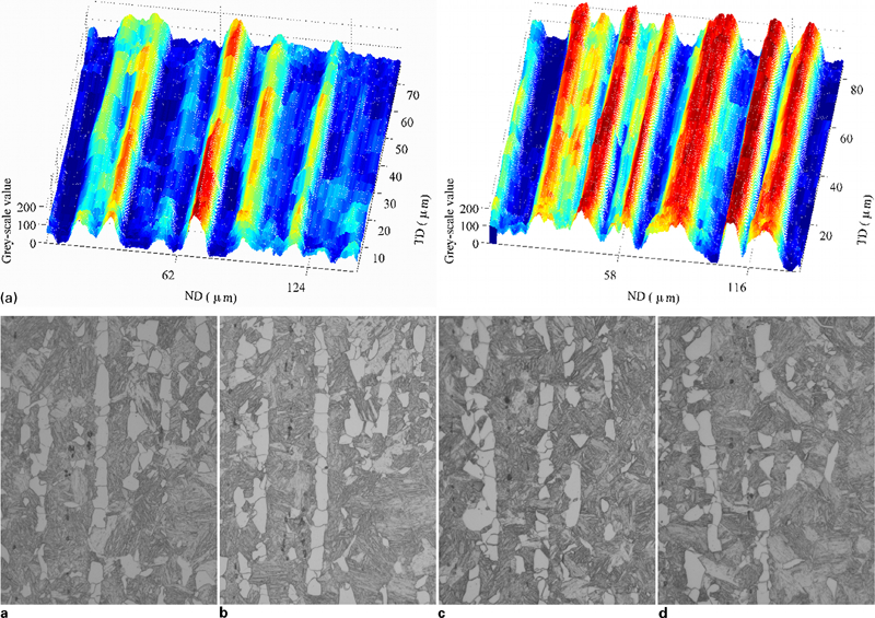
a grey scale profile (row averaged along columns) for all 55 slices in stack (Steel A left, Steel B right) and b–e actual images of steel A normal to RD at various distances (b 0 μm; c 11 μm; d 59 μm; e 76 μm) in TD (normal direction, →; rolling direction, ↓)
Observing the stacked profiles for steel A (left plot Fig. 3a) and the images of the microstructure at various sectioning depths (Fig. 3b–e), several conclusions can be drawn about the behaviour of the ferrite bands in the direction of the sectioning. First, the strongest peak of the profiles is found in the centre ∼70 μm, and it remains the strongest through the sectioning direction. This corresponds to the obvious band in the centre of the optical micrographs, which remains visible, but towards the end of the sectioning depth appears to break into pieces corresponding to the slightly lower amplitude in the profiles. In contrast, while the peaks at ∼14 and 30 μm remain through the TD with only small changes in position and width, they appear to merge together to form one larger band and then break apart again to form two bands at various locations in the depths. This behaviour can also be seen in the micrographs. Finally, looking at the peaks at ∼95 and 120 μm, they appear to start and end in the sectioning direction, which is also supported by the micrographs. From this, it is reasonable to conclude that these peaks really do represent the bands observed in the actual images for various slices.
Now, conclusions can be drawn for steel B without necessarily needing to see the actual microstructure. The profile for steel B is the right hand plot in Fig. 3a. For this material, it appears that all of the bands are strong through the entire depth of the material. Unlike steel A, it appears that some of the bands shift their centre positions, giving a slightly wavy look to the bands in the depth. Like steel A, there is a band centred near 30 μm that appears to split into two bands in the sectioning depth. From these simple grey scale profiles, significant qualitative information about the 3D nature of the bands may be obtained.
Band connectivity
Connectivity plays an important role in the mechanical properties of steel. Information about connectivity is completely lost when only a 2D image is considered. There, using the stylised bands, as defined in the section on ‘Threshold banding’ and shown in Fig. 2b, the connectivity of the bands in the direction of sectioning is explored.
Since the stylised bands are uniform along the RD, a single value, the vertical centre position C(Bn) of each band Bn provides a unique label for each band. Using C(Bn), the bands can be tracked through the TD to observe the behaviour in 3D. A breadth first search was carried out on the stylised bands to ascertain how connected they are through the transverse (sectioning) direction. Figure 4 shows this connectivity, with each symbol representing a single, connected band through the sectioning direction. This figure is important because it demonstrates the problem of relying on a single 2D image for characterising and quantifying banding in the 3D microstructure. The connectivity of the bands is lost in any given 2D image. For steel A, this is evident when observing the bands centred between 20 and 30 μm. The band near 20 μm appears to be three different bands in the depth. This information is completely lost, especially if comparing images taken at, say, 10 and 50 μm depths. It would not be obvious that these two bands are not the same even though they appear in the same location. On the same token, comparing images taken at, say, 50 and 70 μm, information about the connectivity of the bands is lost. The same can be said about the bands centred between 20 and 40 μm for steel B.
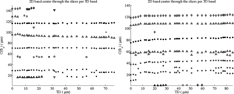
Centre position C(Bn) along ND of images for each band Bn followed through TD (the serial sectioning): symbols correspond to individual bands that are connected through sectioning (steel A, left; steel B, right)
Figure 5 shows 3D images of both steel A (upper images) and steel B (lower images) looking into the depth of the sectioning direction. These images were created by the ImageJ 3D viewer plug-in23 as implemented in the Fiji software.21 These images confirm what was concluded with the stylised bands. The connectivity in 3D is different than what is observable in 2D. For example, in steel B, the pair of bands at the bottom of the images is seen to be connected in 3D while they appear unconnected in many of the 2D slices.
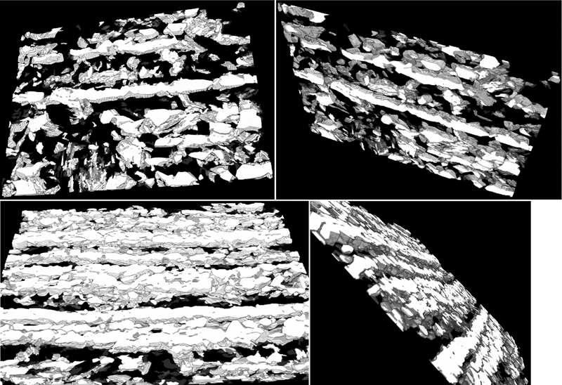
Rotated views of 3D reconstructions from first 24 slices (12 μm into depth) of steel A (top images) and steel B (bottom images). Ferrite bands appear less structured in steel A than in steel B. Much of ferrite does not obviously contribute to band, making steel A arguably weakly banded. Opposite is true for steel B
Three-dimensional banding quantification
In the companion publication,7 two parameters were constructed to quantify banding in microstructures. The band continuity index Cb and the perpendicular continuity index Cp quantify the degree of banding on a bounded scale of [0,1], with 0 indicating no banding and 1 indicating strong banding. Full details of the calculation of these values can be found in Part I,7 but an abridged description of each parameter is given along with the corresponding 3D parameter.
The 2D band continuity index  shown in Fig. 6a is found for each band in the following way


a two-dimensional band continuity index
for each of 55 slices for both steels and b 3D band continuity index  for entire microstructure. Average value is given in each plot and is represented by solid line. Two-dimensional and 3D values for Cb differ slightly, but within set of standard deviations, they could be considered to be same. For both sets of figures, steel A is on left and steel B is on right
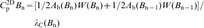
A particle is defined to be a set of grains that has only intraphase grain boundaries. When Cb is one, the band consists of a single particle of the banded phase that fills the entire band region. As Cb approaches zero, either the band is made up of many discontinuous particles, the band area fraction is approaching zero, or both. The more particles there are, the more the banded phase is interrupted by the background matrix phase. This has a direct impact on the strength and ductility of the material, as discussed in the companion paper.7 The 3D band continuity index  shown in Fig. 6b is found for each 3D band in the following way

While this conclusion is perhaps unsurprising, it is useful. The equality of the area and volume fractions has been well established.8,9 However, the contiguity of the phase is not necessarily constant in 3D. It could be that any one slice significantly over or under represents the connectivity of the banded phase, but without explicitly testing this, it is impossible to know for certain. The fact that the 2D and 3D quantification results are essentially equivalent confirms two things. First, this verifies that Cb is reasonable and useful. Second, it confirms the assumption that 2D banded image accurately reflects the 3D banded microstructure.
The 2D perpendicular continuity index Cp shown in Fig. 7a is calculated in the following way

a two-dimensional perpendicular continuity index
for each of 55 slices for both steels and b 3D perpendicular continuity index  for entire microstructure. Average values are given in each plot and are represented by lines. Solid line corresponds to calculating average of
  values for each band over set of stacked images, and dashed line corresponds to calculating
  from band width and centre to centre distances for given band averaged over stack of images. Two-dimensional and 3D values for Cp differ slightly, but within set of standard deviations, they could be considered to be same. For both sets of figures, steel A is on left and steel B is on right
As discussed earlier, due to the connectivity, sometimes what is shown as two separate bands in 2D is really one band in 3D. This makes the 3D value much more difficult to determine than in 2D. Figure 7b shows  calculated in two different ways. The first way is to calculate
  on each 2D image using the 3D connectivity of the bands. If two adjacent bands are actually connected in 3D, then both bands are considered as one in the calculation. This affects the determination of both W(Bn) and λC(Bn). Then, for each band, the value is averaged over the slices. The second way to calculate
  is to first calculate the average widths and centre to centre distances of each 3D connected band from the set of 2D slices, and then to use these average values to calculate
  . The crosses in Fig. 7b show the results for this calculation. While these two methods yield slightly different values, as of yet, there is no reason to choose one method over the other, and so both have been included in this analysis.
From Fig. 7, it can be concluded that for either method of calculating  , the results again confirm that the 2D is reflective of the 3D behaviour despite the fact that the band connectivity is different. Again, this result may not be surprising, but it is significant both with respect to the implications for these banded microstructures and for the utility of the parameters themselves.
Conclusion
The 3D nature of the microstructure bands in two dual phase steels, as observed from serial sectioned optical micrographs, has been presented. Much can be assumed about the behaviour of the bands in 3D from only 2D images, as expected from the extensive studies of random microstructures. However, the connectivity of the bands is neither directly nor accurately observable in 2D images. It is necessary to have knowledge of the full 3D structure to be able to draw conclusions about the material that are based on connectivity or contiguity.
Two parameters that were developed in the companion paper7 have been extended to 3D. It is shown that these parameters yield results in 2D and 3D that are within one standard deviation. This is enough for these values to be reasonably considered the same. While this conclusion is perhaps not surprising, it is important. Since these two parameters, in essence, describe the contiguity of the banded phase in the direction of the band Cb and the contiguity between adjacent bands Cp, the values calculated from a single 2D image reasonably represent what is expected of the 3D image. The validity of these parameters has been established through this. The power of these parameters is that they are defined on a global scale, over the interval [0,1], and so microstructures can be assessed and categorised without needing a direct comparison between two structures. Now, it has been established that these parameters are useful for assessing the full 3D microstructural banding.
Footnotes
Acknowledgements
The present research was carried out under project no. M41·10·09330 in the framework of the Research Program of the Materials innovation institute M2i (![]() ). Thanks to our industrial partner, Tata Steel Europe (formerly Corus Steel), for the materials and the use of the polishing, etching and microscope labs. Thanks to the Metallography and Surface Analysis Group at Tata Steel RT&D for the use of their facilities, help with the data acquisition and for the insightful discussions about the present work. K. S. McGarrity would like to thank E. McGarrity for discussion and help with revising the manuscript. The authors thank K. de Moel, K. Lammers and P. Kok for discussions, guidance and valuable insights with this project. K. S. McGarrity extends special thanks to J. Wörmann for the personal help during the data acquisition period.
). Thanks to our industrial partner, Tata Steel Europe (formerly Corus Steel), for the materials and the use of the polishing, etching and microscope labs. Thanks to the Metallography and Surface Analysis Group at Tata Steel RT&D for the use of their facilities, help with the data acquisition and for the insightful discussions about the present work. K. S. McGarrity would like to thank E. McGarrity for discussion and help with revising the manuscript. The authors thank K. de Moel, K. Lammers and P. Kok for discussions, guidance and valuable insights with this project. K. S. McGarrity extends special thanks to J. Wörmann for the personal help during the data acquisition period.