Modelling dissolution of precipitates considering overlapping of solute fields

Abstract

Upon isothermal dissolution of precipitates, the transformation is controlled by solute diffusion, where the overlapping of diffusion fields in front of the precipitate/matrix interface plays an important role. Analogous to a published model for soft impingement in isothermal precipitation, the dissolution process is classified as two stages: one without and one with overlapping of diffusion fields. In the current modelling, linear approximation for the concentration gradient and equilibrium approximation at the interface are assumed, which allow an analytical description for this kinetic process. The model was first demonstrated by numerical calculation. Then, model predictions were performed for θ′ dissolving in Al–3·0 wt-Cu alloy and Al₂Cu dissolving in Al–4·2 wt-Cu alloy; good agreement with the published experimental data was achieved.

Keywords

Dissolution Precipitate Diffusion controlled Diffusion fields overlap

Introduction

Upon material processing, such as solution treatment, homogenisation treatment, etc., dissolution of precipitates dispersed in solid solution alloys, as a particular diffusion controlled phase transformation in contrast with precipitation, is of great impact on the physical and chemical properties of materials. Compared with flourishing studies of the precipitation from supersaturated solid solution, however, corresponding works on the dissolution of precipitates were relatively few.

In 1961, Thomas and Whelan1 proposed the kinetics of dissolving second phase during solution treatment for Al–Cu alloy. Later, Aaron2 and Whelan3 derived a basic solution model where the dissolution process was found not only to be simply a reversed process of precipitation but also involving a series of complex mathematical description. For example, a precisely quantitative description for dissolution was obtained by solving diffusion equations.4^–7 Without considering the interactions of diffusion fields due to various precipitates, the above models were limited to prediction of the dissolution of one single particle in an infinite matrix.

Upon dissolution of precipitates, the solute atoms are transferred from solute enriched second phase into the matrix. With the diffusion proceeding, the solute concentration of the matrix is varied, which affects the subsequent dissolution. Using stationary interface approximation, Nolfi et al.8 studied the dissolution of a finite array of spheres and solved the diffusion equations by a series expansion. Considering the overlapping of diffusion fields, Tundal and Ryum9 simulated numerically the dissolution process and then described the corresponding experiments for Al–Si alloy10 at high temperatures. For the dissolution of spherical particles in finite media, a semianalytical model was established by Vermolen et al.11 By a diffusional analogue of the heat balance integral method, Asthana and Pabi12 presented an approximate solution for the diffusion controlled dissolution of spherical precipitates. However, it can only describe the real process qualitatively.

As mentioned above, some of the previous models1^–7 do not consider the interactions of diffusion fields of precipitates upon dissolution, while some of them8^–12 consider basically that the interactions are numerical or qualitative, which are inconvenient for direct application. As for the precipitation process, which is closely related with the dissolution process, however, many numerical and analytical models13^–19 have been proposed. Applying an analogous treatment for the overlapping of diffusion fields in precipitation,13 i.e. equilibrium approximation at the interface and linear approximation for concentration gradient, it is herein aimed to establish an analytical model to describe the transformed fraction versus the time in dissolution process, considering the overlapping of diffusion fields.

Model derivation

Basic assumptions

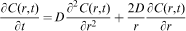
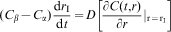
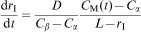
A homogeneous distribution for precipitates with similar sizes is supposed. As for a diffusion controlled dissolution process, thermodynamic equilibrium is assumed to be always established at the particle/matrix interface, i.e. the solute concentrations in both precipitate and matrix remain constant. Therefore, a classical diffusion equation, for diffusion controlled dissolution, follows20 (1) where the concentration distribution C(r,t) is a function of the distance from the centre of the precipitate r and the transformation time t. In isothermal transformation, the diffusion coefficient D can be treated as a constant. Since the precipitate is mostly an intermetallic compound whose solubility changes little with temperature, the current model will not consider the change in solute concentration. Accordingly, the law of solute conservation at the interface leads to20 (2) where r_I represents the distance between the centre of precipitate and the interface front, i.e. the radius of precipitate in the dissolution process. C_β and C_α represent the equilibrium solute concentrations of the second phase β and the matrix at the interface respectively. As indicated in Fig. 1, at low temperature T₀, the average solute concentration is C₀, corresponding to the precipitate with solute concentration as C_β and the matrix with solute concentration as C_M. When heated to solution treatment temperature T, the precipitate gradually dissolves into the matrix. Then, C_α represents the equilibrium solute concentration of the matrix at the interface.

Figure 1

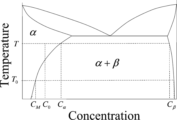
Schematic diagram for dissolution process: when temperature changes from T₀ to T, alloy enters single phase region from two-phase region and precipitates whose solute concentration is C_β dissolve into matrix

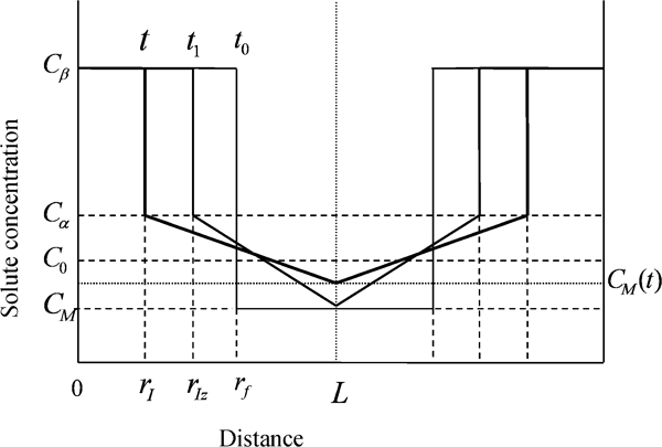
Regarding the homogeneous distribution of precipitates in the matrix, a relationship between the solute concentration and the location is shown in Fig. 2a, where r_f is the initial radius of the precipitate, and L is the middle position of two precipitates (3) with ζ = (C₀−C_M)/(C_β−C_M) as the saturation degree. The above graph in Fig. 2a shows the solute concentration profile at the beginning of dissolution (t = 0), while that below shows that during dissolution (t>0). It indicates that the radius of the precipitate decreases gradually during dissolution. However, in the precipitation process, the radius of the precipitate increases gradually, as shown in Fig. 2b, where C_β′ and C_α′ represent the equilibrium solute concentration of the precipitate and the matrix at the interface. C_M′ is the saturated solute concentration before transformation. r_f′ is the radius of the precipitate when the transformation is completed, and L′ is the middle position of two precipitates. Therefore, we can get that during the dissolution process, the radius of precipitates decreases gradually and the solute transfers from the precipitates to the matrix, while during precipitation, the radius of precipitates increases and the solute transfers from the matrix to the precipitates.

Figure 2

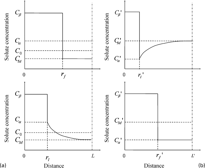
a schematic diagram of relationship between solute concentration profile and distance from centre of precipitate during dissolution process (above graph is for solute concentration profile at t = 0, and below for solute concentration profile at t>0) and b solute concentration profile during precipitation at t>0 and end of transformation

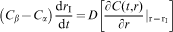
In the process of dissolution, the boundary conditions for equations (1) and (2) are 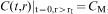, , and r_I(t = 0) = r_f. Actually, an analytical solution to equations (1) and (2) under these boundary conditions is not available. Fortunately, the dissolution rate, the transformed fraction and the kinetic parameters can be obtained numerically. The concentration profiles during dissolution in Al–4·2 wt-Cu alloy, by numerical calculation, are illustrated in Fig. 3. It can be seen that the solute concentration in the matrix gradually increases with dissolving precipitate. The values for the parameters used in the calculation come from Al₂Cu dissolving in Al–4·2 wt-Cu alloy at 546°C:21 r_f = 3 μm, D = 0·1 μm² s⁻¹, C_β = 33 at.-, C_α = 2·24 at.-, C₀ = 1·83 at.- and C_M = 0.

Figure 3

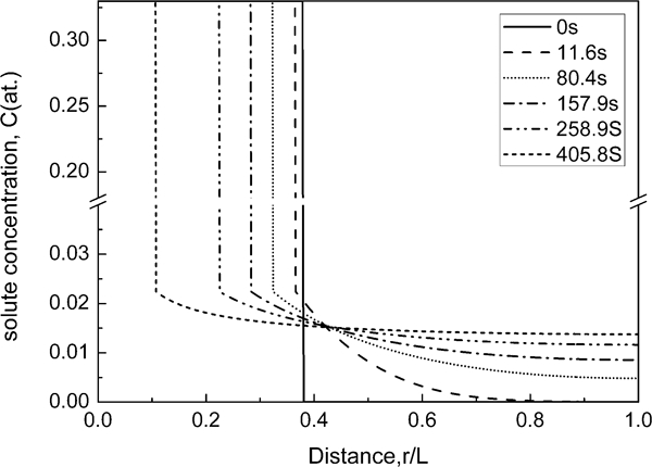
Relationship between concentration profiles and radius of precipitate during dissolution in Al–4·2 wt-Cu alloy at 546°C: profiles are obtained by numerically calculating equations (1) and (2)

Model establishment

A schematic diagram illustrating the dissolution process is shown in Fig. 4, where, analogous to the treatment of soft impingement in precipitation,13 the distance from the centre of precipitate r represents the abscissa, and the solute concentration C represents the ordinate. Suppose the number of precipitate as sufficiently large so that the diffusion fields surrounding the spherical precipitates are supposed to be equivalent at all radial directions, i.e. isotropy at all radial directions holds. At time t = t₀ = 0, r_I = r_f holds; thereafter, r_I decreases, as well as the solute concentration diffusing and overlapping in the matrix. Following the assumption of isotropy and linear approximation for the concentration gradient, the model for dissolution can be classified as the first stage (FS) without the overlapping of concentration fields and the second stage (SS) with the overlapping of concentration fields. In FS, the size of precipitate is larger than the critical size r_Iz, and the diffusion fields are non-overlapping; the dissolution of one single particle in an infinite matrix is dealt with. While in SS, the size of the precipitate becomes less than the critical size r_Iz (the diffusion fields overlap); in the middle position of overlapping, the solute concentration C_M(t) increases gradually with t.

Figure 4

Schematic diagram illustrating dissolution process from non-overlapping to overlapping of concentration profiles. When t = t₀ = 0, radius of precipitate is r_f, i.e. r_I = r_f. In FS, t₀<t<t₁, size of precipitate particle reduces but larger than critical size r_Iz, i.e. r_I>r_Iz, diffusion fields do not overlap. While in SS, t>t₁, size of precipitate particle becomes less than critical size r_Iz, i.e. r_I<r_Iz, diffusion fields overlap. Once radius of precipitate reduces to zero, transformation is complete. In middle position of overlapping, solute concentration C_M(t) increases gradually with time

First stage

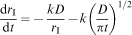
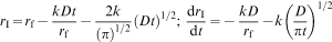
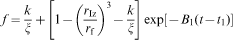
In FS, the diffusion fields of precipitates are non-overlapping. This corresponds to the dissolution of one single particle in an infinite matrix. Equations (1) and (2) were solved by Whelan,3 and the dissolution rate results in (4) where k = (C_α−C_M)/(C_β−C_α). Subjected to the boundary condition, r_I(t = 0) = r_f, analytical relationships for dissolved radius, velocity and time result in (5) Then, the transformed fraction can be given as (6)

Second stage

Analogous to the treatment of soft impingement in precipitation,13 three steps are required in SS:

determining the initial point of overlapping of diffusion fields

describing the evolution of solute concentration in the matrix after the overlapping occurs

iii

deducing the transformed fraction f as function of the transformation time t.

Initial point of overlapping

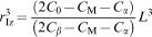
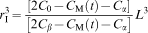
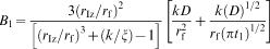
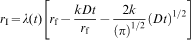
As illustrated in Fig. 4, at the beginning of overlapping, i.e. r_I = r_Iz, a linear approximation and conservation law of mass approximately give13 (7) where g is a particle geometry factor, and r_Iz is the critical radius of overlapping. Rearrangement of equation (7) gives (8) Equation (8) can be used to determine the initial point of overlapping of diffusion fields.

Evolution of solute concentration in matrix after overlapping

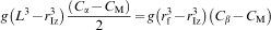
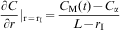
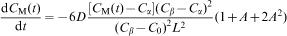
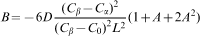
After the overlapping occurs, i.e. r_I<r_Iz, the solute concentration in the middle position of overlapping L increases gradually from the initial value C_M to a time related value C_M(t). According to the conservation law of mass, it is obtained as (9) Rearrangement of equation (9) gives (10) Differentiating equation (10) over t gives (11) The conservation law of solute at the interface20 gives (12) According to the linear gradient approximation (Fig. 4) (13) Then, equation (12) can be rewritten as (14) As for the term 2C_β−C_M(t)−C_α = 2(C_β−C_α)+[C_α−C_M(t)], 2(C_β−C_α) is much larger than [C_α−C_M(t)], so it can be approximated that (15) Combining equations (11) and (14) and using the approximation of equations (15) leads to (16) with A = r_I/L. Since r_I is much less than L, then the value of (1+A+2A²) changes little during SS and can be assumed as a constant.

Given the critical time of overlapping t₁ and the boundary condition for equation (16), C_M(t₁) = C_M, it is obtained as (17) where

Relation between transformed fraction and transformation time

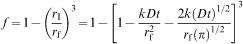
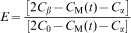
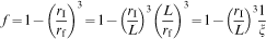
Generally, the transformed fraction is expressed as (18) and then can be obtained by combining equations (10), (17) and (18) as (19) The denominator in equation (19) 2C_β−C_M(t) −C_α can be rewritten as 2(C_β−C_M)−{(C_α−C_M)+[C_M(t)−C_M]}. Since 2(C_β−C_M) is much larger than {(C_α−C_M)+[C_M(t) −C_M]}, 2C_β−C_M(t)−C_α≈2(C_β−C_M) approximately holds. On this basis, equation (19), in combination with equation (15), can be rewritten as (20) where k = (C_α−C_M)/(C_β−C_α); ζ = (C₀−C_M)/(C_β−C_M); t₁ as the critical time when the overlapping happens, i.e. r_I = r_Iz.

In a fixed transformation process, one exact value of transformed fraction f or transformation rate df/dt corresponds to one exact value of time t, i.e. both f and df/dt are continuous during the transformation. Therefore, at the critical time t₁ between FS and SS, f and df/dt are both continuous, i.e. the expression of f should satisfy the following conditions Accordingly, a concise and simple f–t relation in SS can be obtained. 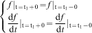Introducing two correction factors C and B₁, we get the correction form of equation (20) (21) Combining equations (21) and (6) and using the above rule lead to (22) where and .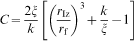

Model description

Uniform expression for dissolution

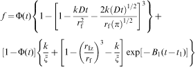
Some previous works8^–12 have discussed the validity of considering overlapping diffusion fields during particles dissolving in a finite matrix. A function of time Φ(t) is proposed to unify the relationship between transformed fraction f and time t in the whole dissolution, including FS without the overlapping of diffusion fields and SS with the overlapping of diffusion fields. Thus (23) where Φ(t) = 1, if t<t₁; Φ(t) = 0, if t⩾t₁.

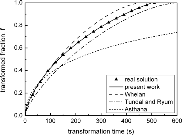
Applying analytical calculations by equation (23) and numerical calculations by equations (1) and (2) with boundary conditions, the f versus t are calculated and illustrated in Fig. 5, where Whelan's model3 without considering the overlapping of diffusion fields, Tundal and Ryum's9 numerical solution and Asthana and Pabi's12 approximate solution are also shown. Since the overlapping of diffusion fields could slow down the process of solute diffusion and the transformation rate, Whelan's model becomes invalid once the overlapping occurs. Although Tundal and Ryum's numerical solution and Asthana and Pabi's approximate solution considered interferences between adjacent particles, the current model resembles more closely the real process. The values for parameters used in the calculation come from Al₂Cu dissolving in Al–4·2 wt-Cu alloy in 546°C:21 r_f = 3 μm, D = 0·1 μm² s⁻¹, C_β = 33 at.-, C_α = 2·24 at.-, C₀ = 1·83 at.- and C_M = 0.

Figure 5

Comparison between current model prediction (equation (23)) and numerical calculations of equations (1) and (2) with boundary conditions, as well as models of Whelan,3 Tundal and Ryum9 and Asthana and Pabi's,12 for fraction transformed upon dissolution at 546°C in Al–4·2 wt-Cu alloy21

Analogous to the soft impingement model in the precipitation process, two stages are used to describe the dissolution process in the current model. The FS and SS are described by equations (6) and (22) respectively. A unified expression for the whole dissolution process is given in equation (23). Although the current model is established following the produce for precipitation model,13 the two models are different. Upon precipitation, as shown in Fig. 6, the growth of precipitate increases the radius of particles but decreases the distance between adjacent particles; the solute transfers from the matrix to the precipitates, and the diffusion fields in front of the precipitate/matrix interface overlap. Upon dissolution, however, the dissolution of precipitates decreases the radius of particles but increases the distance between adjacent particles; the solute transfers from the precipitates to the matrix, and then the diffusion fields of the solute overlap.

Figure 6

Schematic diagram illustrating soft impingement process in precipitation.13 When transformation time t<t₁′, radius of precipitate does not reach r_Iz′, and diffusion fields do not overlap. When t>t₁′, radius exceeds r_Iz′, diffusion fields overlap and solute concentration at intersecting point of diffusion fields changes from C_M′ to C_α′. Once t = t_f′, radius reaches r_f′, and transformation is completed

Time dependent coefficient

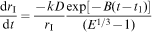
From equation (23), the analytical expressions of f before [i.e. Φ(t) = 1] and after [i.e. Φ(t) = 0] overlapping of diffusion fields are quite different. No mater before or after the overlapping, the dissolution process is always controlled by solute diffusion and not affected by other kinetic parameters, such as effective activation energy Q. Therefore, it will be more accurate if the expressions before and after the overlapping are analogous. Before the overlapping occurs, Whelan's model3 gives a clear description of dissolution, while after the overlapping occurs, now a Whelan-like expression is proposed by introducing a time dependent coefficient.

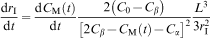
Substitution of equations (10) and (17) into equation (14) gives the dissolution velocity as (24) with Given the boundary condition, r_I(t₁) = r_Iz. Integration of equation (24) gives (25) Introducing a time dependent coefficient λ(t), equation (25) can be rewritten as (26) where (27a) (27b) Therefore, introducing a time dependent coefficient λ(t), the dissolution before and after the overlapping can be expressed as an analogous form, i.e. the current model can be expressed as Whelan's form (28) where if t<t₁, λ^* = 1; if t⩾t₁, λ^* = λ(t).

Model application

Parameter determination

Note that the parameters used in the current model can experimentally be obtained from the initial state of the sample. From the above calculations, several parameters such as r_f, r_Iz, k, t₁, B₁, D and ζ are needed in the current model. The values of r_Iz, k, t₁, B₁ and ζ depend on r_f, D and solute concentrations C_β, C_α, C₀ and C_M. Whereas, values of r_f can be directly obtained from the initial state of the sample, and values of D can be obtained from reference book. Therefore, given r_f, D, C_β, C_α, C₀ and C_M, values for all the parameters can thus be obtained. For a given sample, values of r_f, C_β, C₀ and C_M are determined by the previous precipitation history, whereas values of D and C_α are dependent on annealing temperature T. Therefore, for a given sample and a given annealing temperature, all the parameters can be determined.

Applications

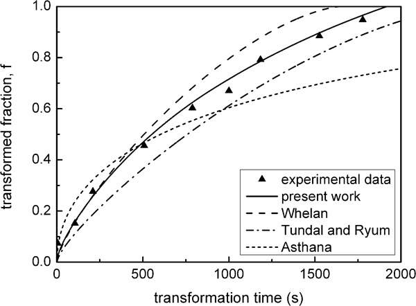
In this section, the current model is adopted to describe the experimental data from Hewitt and Butler22 and Reiso et al.,23 where the dissolution of θ′ in an Al–3·0 wt-Cu alloy and the dissolution of Al₂Cu in an Al–4·2 wt-Cu alloy were studied respectively.

According to Ref. 22, following alloy preparation, the samples were solution heat treated at 550°C for 30 min, water quenched and aged at 285°C for 22 h to produce a microstructure consisting of many precipitate particles of semicoherent θ′. Then, the specimens were examined in an EM7 high voltage electron microscope operated at 500 kV. Observations of the θ′ dissolution process were performed at 370°C. A timed sequence of micrographs was obtained using a data acquisition system, and the area of θ′ at each time step was determined using stereometric analysis software.22 Then, the relationship between the particle radius and the transformation time (i.e. the relationship between f and t) could be obtained, as shown in Fig. 7. Relevant parameters such as r_f, C_β, C_α, C₀ and C_M can be obtained from Ref. 22, and D is obtained from Ref. 24 (see Table 1). According to Ref. 23, the Al–4·2 wt-Cu alloy was produced by directional solidification, then homogenised for 4 days at 530°C and subsequently broken down by cold rolling with intermediate annealing at 430°C. After that, the specimens were annealed for 2 h at 530°C in air. The temperature was then decreased by 1°C h⁻¹ down to 450°C, after which the specimens were quenched in water. To observe dissolution of the Al₂Cu precipitates, a series of up-quenching experiments to 546°C were run. The area fraction of precipitates was measured by means of an interactive image analysis system (IBAS) instrument.23 Dissolution data were digitised using ‘GetData’ software. The transformed fraction of precipitate is shown as a function of time in Fig. 8. The relevant parameters for calculation can be obtained from Ref. 23 (see Table 1). The current model and the models of Whelan,3 Tundal and Ryum9 and Asthana and Pabi12 were applied to describe the above two dissolution processes (Figs. 7 and 8). Obviously, the current model gives more precise prediction to the experimental data than the others.

Figure 7

At 370°C, evolution of transformed fraction f with solution treatment time t in dissolution of θ′ in Al–3·0 wt-Cu alloy. Experimental data are quoted from Ref. 22. Present work is calculated by equation (23). Whelan,3 Tundal and Ryum9 and Asthana and Pabi's12 models are compared as well

Figure 8

At 546°C, evolution of transformed fraction f with heat treatment time t in dissolution of Al₂Cu in Al–4·2 wt-Cu alloy. Experimental data quoted from Ref. 23. Present work is calculated by equation (23). Whelan,3 Tundal and Ryum9 and Asthana and Pabi's12 models are compared as well

Table 1

Parameters used for current model prediction for dissolution of θ′ in Al–3·0 wt-Cu and Al₂Cu in Al–4·2 wt-Cu alloy

References	T/°C	r_f/μm	C_β/at.-	C_α/at.-	C₀/at.-	C_M/at.-	D/μm² s⁻¹
22	370	0·25	0·33	0·00857	0·00627	0	0·000586
24	546	3	0·33	0·0224	0·0183	0·013	0·1

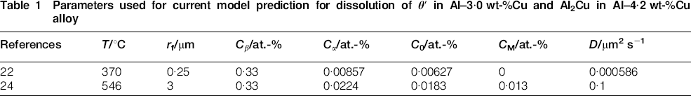
Although the above two dissolution processes both belong to the transformation of Al based alloy, the parameters used to predict the processes must be quit different, arising from the different precipitation histories and different annealing temperatures. In Hewitt's experiment, the supersaturation specimens were aged at 285°C for 22 h to produce a microstructure consisting of many precipitate particles of semicoherent θ′. While in Reiso et al.'s experiment, the specimens were annealed for 2 h at 530°C in air. The temperature was then decreased by 1°C h⁻¹ down to 450°C. Therefore, in the two experiments, the processes of producing the precipitate were different, and the parameters r_f, C_β, C_M and C₀ that describe the precipitate are totally different (see Table 1). Furthermore, owing to the different solution treatments at 370°C for θ′ dissolution and 546°C for Al₂Cu dissolution, values of D and C_α vary significantly, i.e. the higher the T, the large the values for D and C_α.

Conclusions

Analogous to a published model for soft impingement in isothermal precipitation,13 under the assumption of linear approximation for the concentration gradient and equilibrium approximation at the interface, an analytical expression for the isothermal dissolution of precipitates that considered the overlapping of diffusion fields in front of the precipitate/matrix interface was developed. Compared with the numerical solution, it has been shown that the current model can describe the real dissolution process precisely. In addition, the dissolution processes before and after the overlapping of diffusion fields can be expressed as a uniform function (i.e. Whelan's form) by introducing a time dependent coefficient. Then, the current model accurately predicts the isothermal θ′ dissolving in Al–3·0 wt-Cu alloy and Al₂Cu dissolving in Al–4·2 wt-Cu alloy, i.e. the current model is physically realistic.

Footnotes

Acknowledgements

The authors are grateful for financial support of the Free Research Fund of State Key Lab. of Solidification Processing (grant nos. 09-QZ-2008 and 24-TZ-2009), the 111 project (grant no. B08040), the Natural Science Foundation of China (grant no. 51071127), the Huo Yingdong Yong Teacher Fund (grant no. 111052), the Fundamental Research Fund of Northwestern Polytechnical University (grant no. JC200801) and National Basic Research Program of China (973 Program) (grant no. 2011CB610403).

References

Thomas

, Whelan

: Philos. Mag. , 1961, 6, 1103–1114.

Aaron

: Met. Sci. J. , 1968, 2, 192–193.

Whelan

: Met. Sci. J. , 1969, 2, 95–97.

Nojiri

, Enomoto

: Scr. Metall. Mater. , 1995, 32, 787–791.

Aaron

, Fainstein

, Kotler

: J. Appl. Phys. , 1970, 41, 4404–4410.

Aaron

, Kotler

: Metall. Trans. , 1971, 2, 393–408.

Cable

, Frade JR : J. Mater. Sci. , 1987, 22, 1894–1900.

Nolfi

, Shewmon

, Foster

: Trans. AIM , 1969, 245, 1427–1433.

Tundal

, Ryum

: Metall. Trans. A , 1992, 23A, 433–444.

10.

Tundal

, Ryum

: Metall. Trans. A , 1992, 23A, 445–449.

11.

Vermolen

, Mourik

Pvan

, der Zwaag

Svan

: Mater. Sci. Technol. , 1997, 13, 308–312.

12.

Asthana

, Pabi

: Mater. Sci. Eng. A , 1990, A128, 253–258.

13.

Fan

, Liu

, Zhang

, Yang

, Zhou

: Acta Mater. , 2008, 56, 4309–4318.

14.

Clavaguera-Mora

, Clavaguera

, Crespo

, Pradell

: Prog. Mater. Sci. , 2002, 47, 559–619.

15.

Crespo

, Pradell

, Clavaguera-Mora

, Clavaguera

: Phys. Rev. B , 1997, 55B, 3435–3444.

16.

Pradell

, Crespo

, Clavaguera

, Clavaguera-Mora

: J. Phys. Condens. Matter , 1998, 10, 3833–3844.

17.

Tkatch VI , Rassolov

, Moiseeva

, Popov

: J. Non-Cryst. Solids , 2005, 351, 1658–1664.

18.

, Lai

YKL

, Zhang

: J. Appl. Phys. , 1997, 82, 4270–4276.

19.

Wang

, Liu

, Zhang

, Yang

, Zhou

: Acta Mater. , 2009, 57, 3072–3083.

20.

Christian

: ‘The theory of transformations in melts and alloys’; 2002, Oxford, Pergamon.

21.

Durbin

: ‘Modeling dissolution in aluminum alloys’, PhD thesis, Georgia Institute of Technology, Atlanta, GA, USA, 2005.

22.

Hewitt

, Butler

: Acta Metall. , 1986, 34, 1163–1172.

23.

Reiso

, Overlie

, Ryum

: Metall. Trans. A , 1990, 21A, 1689–1695.

24.

Brandes

, Brook

: ‘Smithells metals reference book’; 1992, London, Butterworths.