Prediction of cutting forces and surface roughness using artificial neural network (ANN) and support vector regression (SVR) in turning 4140 steel

Abstract

In the present study, the prediction of cutting forces and surface roughness was carried out using neural networks and support vector regression (SVR) with six inputs, namely, three axis vibrations of the tool holder and cutting speed, feedrate and depth of cut. The data obtained by experimentation are used to construct predictive models. A feedforward backpropagation neural network and SVR have been selected for modelling. The coefficient of determination (R²), mean absolute prediction error and root mean square error were calculated for each method, and these values served as a measure of prediction precision. We carried out comparison of the prediction accuracy of artificial neural networks and SVR. Comparison of the two models indicates that both models have successful performance. Experimental results are provided to confirm the effectiveness of this approach.

Keywords

Neural network CNC turning Surface roughness SVR prediction model

Introduction

Cutting force and surface roughness are key process parameters in metal. For example, cutting force has a significant influence on tool and workpiece deflections in machining. The development of cutting force models is essential for thermal analysis, the prediction of tool life and chatter and tool condition monitoring.

The cutting force is one of the most important characteristic variables to be monitored in cutting processes owing to the direct relation between the change in cutting force and cutting conditions.1 Cutting forces are the basis for the evaluation of the necessary power machining (and choice of the electric motor). They are also used for dimensioning machine tool components and the tool body. They influence the deformation of the machined workpiece, its dimensional accuracy, chip formation and machining system stability.2

Surface roughness is used in evaluating the quality of parts. It also affects several functional attributes of parts, such as leakage, surface friction, wear, light reflection, heat transmission and ability to distribute and hold a lubricant, coating or resistance to fatigue.

Consequently, cutting forces and surface roughness predictions play a significant role in the machining industry for the proper selection and control of machining parameters and optimisation of cutting conditions.

For a long time, researchers have been trying to optimise the performance of metal cutting operations through efficient quantitative and predictive models that establish the relationship between a large set of independent input parameters and output variables. Such models are required for the wide spectrum of manufacturing processes, cutting tools and engineering materials currently used in the industry.3

Because metal cutting mechanics is quite complicated, it is very difficult to develop a comprehensive model that involves all cutting parameters affecting the machining process.

With the advancement in computer technology, the artificial neural network (ANN) has become preferred by many researchers as a robust predictive technique. In recent years, it has become ubiquitous in the modelling of highly non-linear systems, especially in those systems/processes where system dynamics is defined by a large number of variables. The versatility of ANN mostly comes from its capability to learn from past data and to be able to update itself based on errors.

The ANN can monitor tool wear, chatter vibration and chip break during turning for real time fault detection. Rahman et al.4 obtained a fairly high detection accuracy using ANNs.

Samanta et al.5 presented to model surface roughness in end milling using soft computing or computational intelligence techniques. The machining parameters, namely, the spindle speed, feedrate and depth of cut, were used as inputs to model the workpiece surface roughness. The model parameters were tuned using training data maximising the modelling accuracy. They explained the effectiveness of computational intelligence techniques in modelling surface roughness.

The effect of material swelling on the surface roughness in ultraprecision diamond turning had been investigated by To et al.6 Their experimental results showed that the profile of the tool marks was distorted by the effect of swelling of the materials being cut. The deformation induced surface roughness of polycrystalline AA 6022-T4 aluminium was evaluated, which determined the rms roughness R_q with linear roughness profiles to be consistent with literature practice and R_q by matrix methods. The present study indicated that when R_q data were acquired via linear profiles, they were strongly influenced by correlations.7 Lee et al.8 presented a system for measuring the surface roughness of turned parts through computer vision system. The images of specimens grabbed by the computer vision system could be treated by some techniques to get the features of the image texture. Using the trained abductive network, the experimental result had shown that the surface roughness of turned parts measured by the computer vision system over a wide range of turning conditions could be obtained with a reasonable accuracy compared with those measured by the traditional stylus method.

Gupta9 undertook a study to calculate surface roughness, tool wear and the required power dependent on cutting speed, feedrate and cutting time. The obtained data were used to develop models using response surface methodology, ANN and support vector regression (SVR) methods. The results showed that the ANN and SVR models yielded higher accuracy than the response surface methodology model.

Many studies use ANN to monitor and predict surface roughness, cutting forces, tool wear and tool life. However, none of those neural networks and SVR with seven inputs, namely, profile angle, three axes vibrations of the tool holder, cutting speed, feedrate and depth of cut, were found to predict the surface roughness and cutting forces as outputs. Thus, the distinct contribution of the present study is to investigate the effect of profile angle and vibrations, in addition to other commonly used cutting parameters, on surface roughness and cutting forces. The results obtained show that the proposed ANN and SVR models predict surface roughness and cutting forces with a fairly high accuracy when compared to other similar studies described in the literature.

In the present paper, dynamic models for turning are developed to predict the cutting forces and surface roughness. The predictions are validated experimentally for the case of turning of AISI 4140 steel.

Modelling of cutting force

One of the most commonly used cutting force component models for turning is given in Ref. 10 (1) where C is a coefficient that is dependent on the machined material, d is the depth of cut (mm), f is the cutting feed (mm rev⁻¹), V is the cutting speed (m min⁻¹), xp, yp and np are coefficients dependent on the machining type and cutting tool material, K_mp is a coefficient that is dependent on the machined material, K_κ_p is a coefficient that is dependent on the major cutting edge angle, K_Θp is a coefficient that is dependent on the clearance angle, K_λ_p is a coefficient that is dependent on the major cutting edge inclination angle λp, K_rp is a coefficient that is dependent on the tool nose radius r and K_VBp is a coefficient that is dependent on the average cutting tool flank wear VB. This equation is based on statistical analysis of machining data, obtained via changing one or more machining parameters, while the others are fixed. An obvious drawback of this model is that xp, yp, np, K_mp, K_κ_p, K_Θp, K_λ_p, K_rp and K_VBp are considered constants. To take the mutual effect of the cutting parameters into account, a large number of cutting force models have been developed.

In Ref. 11, the influence of cutting feedrate and depth of cut on xp and yp is expressed by the following relationship (2) where K_mp, K_κ_p, K_Θp, K_λ_p, K_rp, K_VBp, k and m are coefficients. Whatever analytical models are used, they can hardly cope with the complexity of the cutting process. Moreover, for developing an analytical model, proper methods for extracting general relationships from existing machining data are required.

The depth of cut, feed and cutting speed represent the machining settings, which can easily be established in any turning operation. Experiments can reveal the influence of these parameters on the cutting forces. However, experiments are expensive and time consuming. An empirical relationship can be used as alternative to traditional methods. Based on experience, some constant exponents of the parameters are chosen/estimated in these relationships. The choice of the exponents is subjective. Moreover, it is difficult to relate the choice of these exponents to the changing cutting conditions. The aim is to develop a generalised model based on measured forces under actual machining conditions, which is then used for predicting the output for the unknown input parameters.12 In the present study, experiments were conducted to measure cutting force (Fx), passive force (Fy), feed force (Fz) at different feedrate, cutting speed, profile angle and depth of cut.

Modelling of surface roughness

Based on ISO 4287 norm, the average surface roughness R_a can be defined as the arithmetic mean of the deviations of the roughness profile from the central line lm along the measurement.13^–15 This definition is given in equation (3) (3) where L is the sampling length of the profile, and y is the coordinate of the profile curve. The relationship between surface roughness and cutting parameters can be defined in equation (2) (4) where R_a is the arithmetic average surface roughness (μm). V, f, a and r are the cutting speed (m min⁻¹), feedrate (mm rev⁻¹), depth of cut (mm) and tool nose radius (mm) respectively. C, n, m, p and l are constants, and ϵ is a random error. In order to distinguish constants and parameters in the equation, equation (3) is expressed as in equations (5)and (6). The surface roughness of turned surfaces defined by Ra and Rt can be computed as follows15,16 (5) (6) Equations (5) and (6) show that while the surface roughness proportionally increases with the feedrate, a large tool nose radius reduces the surface roughness of a turned work piece. Imperfections caused by tool vibration and chip adhesion are not considered in this model.

Experimental

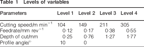
Tests were carried out using a 12 speed Jones and Lamson Lathe. The specimen with a diameter of 60 mm and a length of 500 mm was hardened to 35 HRC. The cutting tool (DTGNR 163 C 0° Lead Angle 60° Triangle insert), which was used to carry out the cutting tests, was a commercial product available from the Kennametal Company. Carbide inserts with product number Tips TNMG 080408 MN/FN CVD TiCN and a thick α-Al₂O₃ CVD coating were used. Cutting parameters, i.e. cutting speed, cutting depth and feedrate, were suggested by the cutting tool supplier and finally selected, as shown in Table 1. Four different levels were considered for each of the four parameters, and a total of 128 experimental runs were carried out, one for each possible combination of parameter values.

Table 1

Levels of variables

Parameters	Level 1	Level 2	Level 3	Level 4
Cutting speed/m min⁻¹	104	149	211	305
Feedrate/mm rev⁻¹	0·12	0·17	0·38	0·55
Depth of cut/mm	0·25	0·76	1·27	1·77
Profile angle/°	10	0

The force measurements were acquired using a Kistler three-axis dynamometer attached to the workpiece holder. The dynamometer (model 9257B) was tested with the original Kistler evaluating technique, so in this case, the calibration sensitivity of Fx, Fy and Fz was used, as received from the manufacturer, to set-up the transducer sensitivity of the charge amplifiers (model 5011A). The accelerometer sensor used was a K-Shear triaxial accelerometer type 8792A, which was mounted on the shank of the tool holder, directly above the cutting tool. The axes of the accelerometer were aligned with the axes of the lathe (X, Y and Z). The data acquisition card was a National Instruments portable E Series NI DAQ Card-6036E with maximum acquisition rate of 200 000 samples/s. The data were acquired with ASILTURK_DAQ_V2. This software was developed using Matlab 6·5 software. Outputs were measured as 80 samples/s, and their average values were recorded as one datum. The experimental set-up is shown in Fig. 1.

Figure 1

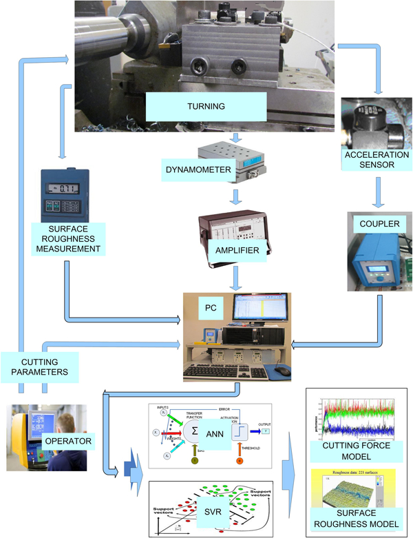
Experimental set-up

A roughness tester (TR100) was used to measure the surface roughness (Ra and Rz) after each grinding operation. For each sample, three readings, 120° apart, were taken. The average is used as a measure of roughness of the surface resulting from turning. In order to eliminate the effect of tool wear, each experiment was performed with a new cutting tool.

Artificial neural network and SVR

An ANN model consists of at least three layers of neurons, namely, input layer, hidden layer and output layer. Figure 2 shows the components of a neuron.

Figure 2

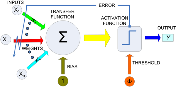
Components of neuron17

The ANN maps input space to output space and is trained to minimise the error between the predicted and actual output values. Input samples are characterised by a numeric feature vector. Input and output pairs available in the training data are provided to ANN one by one, and ANN updates the weights at each node to minimise the mean square error. This process is known as training, and it continues until the termination criterion is met. The termination criterion is usually defined by the maximum number of iterations or the change in error between any two iterations. Once the training is completed, ANN can be used to predict the outputs of new samples. This process is known as testing. The most commonly used algorithm for training ANNs is backpropagation. More detailed information concerning ANNs can be found in the literature.17^–19

A support vector machine (SVM) is a supervised learning method that is used for classification and regression analysis. When SVM is applied to regression estimation problems, it is referred to as SVR.20

In SVR, the main goal is to find a function f(x) that has at most ϵ deviation from the obtained targets for all the training data and at the same time is as close as possible. The model produced by SVR depends only on a subset of training data, because the cost function for building the model ignores any training data close to the model prediction (within a threshold).21

Results and discussion

In this section, the results obtained from SVR and ANN are compared and discussed. The dataset is partitioned into a training set and a testing set. The training set contains 90 samples. The remaining 37 samples are used for testing.

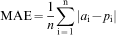
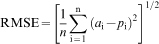
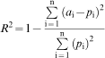
It is easy to estimate that there may be some differences between measured and predicted values. This difference can be quantified by statistical measurements. In the present study, the mean absolute error (MAE), root mean square error (RMSE) and coefficient of determination R² has been used. The formulas for the calculation of MAE, RMSE and R² are as follows (7) (8) (9) where a_i is the actual value and p_i is the predicted value.

To design the model, the first step is to normalise the input and output values in the range [0, 1].

The normalisation is conducted as follows (10) Ten different models were designed. Five models were designed using ANN, and the other five using SVR method for Ra, Rz, Fx, Fy and Fz (see Table 2). Same samples were split for training and testing parts for all 10 models. All models have six inputs, namely, three axes vibrations of the tool holder, cutting speed, feedrate and depth of cut. The optimum number of neurons for ANN is determined by gradually increasing the number of neurons (a maximum of 15 neurons is considered) and then choosing the number with the minimum mean square error.

Table 2

Obtained statistical results for testing parameters

	ANN				SVR
	RMSE	MAE	R ²	Slope	RMSE	MAE	R ²	Slope
Ra	0·0568	0·0371	0·9817	1·0068	0·0598	0·0315	0·9783	0·9724
Rz	0·0950	0·0624	0·9498	1·0005	0·0975	0·0519	0·94	0·9353
Fx	0·0704	0·0561	0·9705	0·9669	0·08	0·0532	0·9528	0·8676
Fy	0·1271	0·0931	0·9045	0·9503	0·0801	0·0622	0·96	0·938
Fz	0·0835	0·067	0·9685	0·9515	0·0757	0·0516	0·9747	0·935

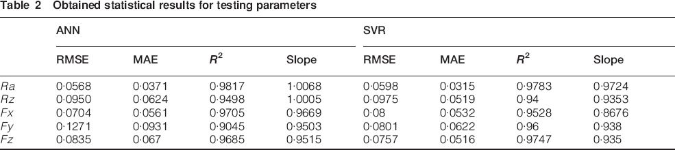
After various trials, the three-layer network with three neurons in the hidden layer was determined as the best ANN model for the Ra parameter. The learning rate was 1. LibSVM 2·91 was used to design the SVR model. As a result, a value of 54 for totals was obtained. Comparing the results of statistical measurements (see Table 2) and the distribution of points in Fig. 3, it can be claimed that both models show equal performance to predict Ra.

Figure 3

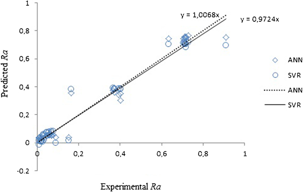
Correlation between experimental and predicted Ra values by ANN and SVR

To create a model for the Rz parameter using ANN, a three-layer network with two neurons in the hidden layer was determined as the most successful. The learning rate was 0·7. For SVR, a value of 55 for TotalSV was obtained. Comparing the results of statistical measurements (see Table 2) and the distribution of points in Fig. 4, it can be observed that although the SVR is successful to predict the Rz, the ANN is a bit better (see slope and MAE).

Figure 4

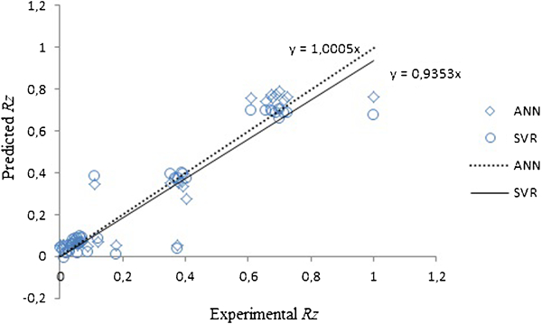
Correlation between experimental and predicted Rz values by ANN and SVR

To model Fx with ANN, the three-layer network with nine neurons in the hidden layer was determined as the most successful. The learning rate was 0·7. For SVR, a value of 50 for TotalSV was obtained. Comparing the results of statistical measurements (see Table 2) and the distribution of points in Fig. 5, it can be seen that ANN is better than SVR.

Figure 5

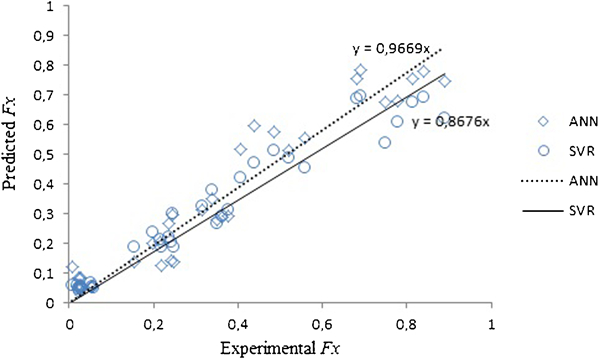
Correlation between experimental and predicted Fx values by ANN and SVR

For Fy, the three-layer ANN model with nine neurons in the hidden layer was identified as the most successful. The learning rate was 0·4. For SVR, a value of 52 for TotalSV was obtained. Comparing the results of statistical measurements (see Table 2) and the distribution of points in Fig. 6, it can be clearly seen that SVR is more successful in predicting Fy than ANN.

Figure 6

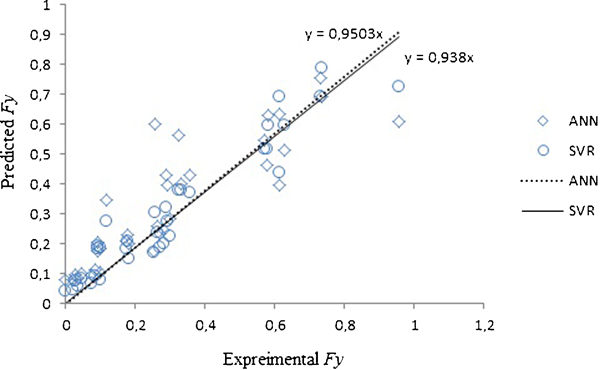
Correlation between experimental and predicted Fy values by ANN and SVR

For Fz, the three-layer ANN model with 10 neurons in the hidden layer was determined as the most successful. The learning rate was 1. For SVR, a value of 54 for TotalSV was obtained. Comparing the results of statistical measurements (see Table 2) and the distribution of points in Fig. 7, it can be clearly seen that SVR is more successful in predicting Fy than ANN.

Figure 7

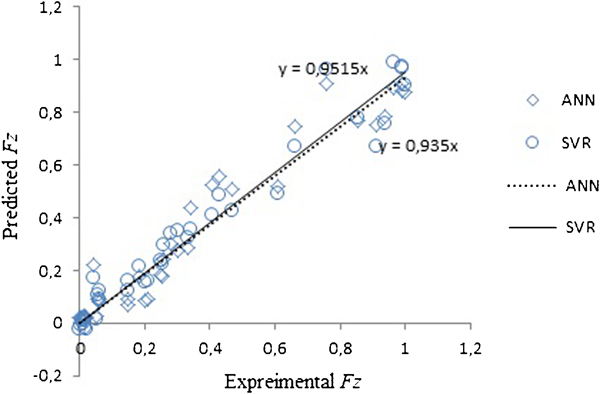
Correlation between experimental and predicted Fz values by ANN and SVR

As seen from the above mentioned statistical measures, the obtained results for both methods are very close to the desired ones. Figure 8 shows the comparative results of ANN, SVR and experimental results. As can be seen from these figures, both models are successful.

Figure 8

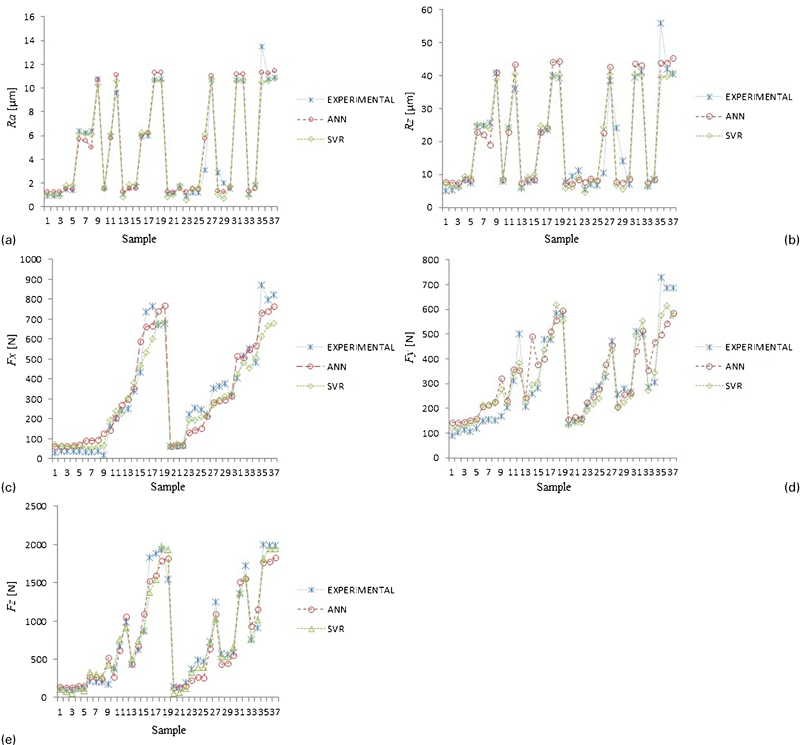
Comparison of experimental and predicted by ANN and SVR

Comparison of the two models indicates that the prediction model developed by the SVR is more accurate than that developed by ANN. Experimental results are provided to confirm the effectiveness of this approach.

Conclusions and future research

The present investigation is concerned with predicting the surface roughness and cutting force based on the vibrations of the tool holder and insert profile angle. Two predictive models based on ANN and SVR respectively are developed for that purpose. The process parameters considered here are feedrate, cutting speed, profile angle, tool holder vibrations and depth of cut. The tool profile angle and vibrations were included in the models in order to obtain higher prediction accuracy.

The results obtained using the ANN and SVR models are compared. Considering the negligible error rate achieved as well as the advantages of learning and practicality in terms of speed and capacity, the developed SVR model can be successfully recommended and deployed for practical (industrial) application.

The ANN model gave overall 0·0631 MAE and 0·0501 RMSE, while the SVR model gave 0·0898 and 0·0795 of MAE and RMSE respectively. R² has been found as 0·9013 for ANN, while it is equal to 0·9273 for SVM. The slopes are 0·9616 and 0·93 for ANN and SVR respectively.

This has been shown to be especially true for complicated, highly non-linear objects/systems.

Footnotes

Acknowledgements

The present study was supported by Scientific Research Projects Coordinators (BAP) of Selcuk University, IUPUI and TUBITAK.

References

Kassab

: Proc. Int. Conf. on ‘Modeling and simulation estimation of cutting force in turning operation from measurement of motor current’, Konya, Turkey, August 2006, Selcuk University, Paper 113.

Fnides

, Aouıcı

, Yallese

: Mechanika , 2008, 2, 70–75.

El-Hosseina

, Kadirgama

, Hamdib

, Benyounis

: J. Mater. Process. Technol. , 2007, 82, (1–3), 241–247.

Rahman

, Zhou

, Hong

: Int. J. Adv. Manuf. Technol. , 1995, 10, (2), 87–92.

Samanta

, Erevelles

, Omurtag

: Proc. Inst. Mech. Eng. B: J. Eng. Manuf. , 2008, 222, (10), 1221–1232.

, Cheung

, Lee

: Mater. Sci. Technol. , 2001, 17, (1), 102–108.

Stoudt

, Hubbard

, Janet

: Mater. Sci. Technol. , 2008, 24, (3), 253–260

Lee

, Yu

, Juan

: Mechatronics , 2004, 14, (1), 129–141.

Gupta

: Int. J. Manuf. Technol. Manage. , 2010, 48, 763–778.

10.

Kosilova

: ‘Manufacturing handbook’, Vol. 2, 347–356; 1985, Moscow, Mashinostroene.

11.

Szecsi

: J. Mater. Process. Technol. , 1999, 92–93, 344–349.

12.

Kumanan

, Nanne

: J. Inst. Eng. (India) , 2006, (87), 11–15.

13.

Stephenson

, Agapiou

: ‘Metal cutting theory and practice’, 2nd edn; 2005, New York, CRC Press.

14.

Nalbant

, Gokkaya

, Toktas

: Model. Simul. Mater. Sci. Eng. , 2007, 2, 14.

15.

Sahin

, Motorcu

: Int. J. Refract. Met. Hard Mater , 2002, 26, (2), 84–90.

16.

Liou

, Kuo

: ‘Data flow design for the backpropagation algorithm’, Proc. Int. Computer Symp., Taipei, Taiwan, Selcuk University, December 2002, 1–5.

17.

Topal

: Int. J. Mech. Sci. , 2009, 51, (11–12), 782–789.

18.

Ozdeniz

, Yilmaz

: Energy Sources A , 2009, 31A, 1425–1435.

19.

El-Hossainy

: Mater. Manuf. Process. , 2010, 25, (12), 1505–1512.

20.

Juang

, Hsieh

: Fuzzy Sets Syst. , 2009, 160, 2486–2504.

21.

Basak

, Pal

, Patranabis

: Neural Inf. Process. Lett. Rev. , 2007, 11, (10), 203–224.