Non-linear partial least squares and its application to minimising scale formation at a steel hot mill

Abstract

Scale is highly detrimental to surface quality for tinplate products. As there are a large number of process variables at a typical hot mill, non-linear partial least squares was used to study the influence of these process parameters on tertiary scale formation. It was found that a logit model containing just two partial least squares components provided an adequate best fit to the process data with the most significant variables being the average temperatures at which the steel strip was entering the finishing and rolling mills, the average crop shear temperature and the percentage of phosphorus present within the strip.

Keywords

Hot mill Logit model Partial least squares Scale

Introduction

For high end flat steel products, scale is clearly detrimental to surface quality. Scale is formed at the hot mill but it has its greatest impact on quality after further processing. Scale can have a particularly negative impact on quality for tinplate products. This occurs due to the scale interfering with the interface between the steel substrate and the tin, resulting in a product surface that is not suitable for the tight tolerances required by customers of tinplate products. While it is well known which process variables are the major determinants of scale formation (for example, phosphorous and temperature), it is less well known at precisely which levels to set these important variables so as to minimise the chances of scale forming at the hot mill. While this information is very important for maximising the number of rolled coils that can be used for high end applications, quantifying these values for the key process variables is complicated by the fact that there is more than one temperature at the hot mill that could influence scale, and more importantly, these temperatures are highly correlated with each other, making it difficult to disentangle their individual contributions to scale formation.

This paper will use a PLS model to identify not only what the important chemistries and temperatures are, but also the numerical effect of changing these processing parameters on the quantity on scale forming at the hot mill. With so many different temperature variables, this technique is used to reduce data dimensionality and hence the correlation between these process variables. The aim is not just to identify the important temperature variables but more importantly to find what temperature values and chemical additions should be avoided when trying to produce high end sheet steel.

Data mining techniques have been used in the past to investigate scale defects using analytical techniques proposed by Haapamaki et al.1 and Haapamaki and Roning.2 It was concluded by these authors that such data analysis was possible but only if high frequency data were used. This paper will use over 1500 records of the same steel grade and same gauge (thickness) to minimise the effects of processing conditions. Owing to the influence of scale on further processing, the best way of minimising the impact of scale is by understanding the influence of process variables at the hot mill. This will then enable control engineers to set the process variables at levels that minimise the formation of scale.

Literature review on scale type and formation

Scale

Scale is an oxide layer that builds up on the surface of the steel when it is exposed to environmental conditions. Oxide can form at any point during the life cycle of the product; however, it is particularly likely to occur at the hot mill. This is due to the high temperatures at the hot mill, which increases the speed of any chemical reaction. Bolt3 states that the important properties to consider for the oxide layer are thickness, composition, adhesion and structure. Bolt3 also mentions that structure and cohesion are of importance to scale formation, but that these properties are of less importance.

The thickness of the oxide layer will be determined by its processing conditions. Bolt3 states that the most important parameters for thickness are the finishing temperature and gauge of the coil. Depending on the temperature of the strip, oxide could be formed at the run-out table (ROT) and also during coiling but that scale formation at these stages is rather modest. Bolt3 also concludes that thickness is of particular importance to pickling lines, because the thicker the oxide is, the easier it is to promote cracking. This is supported in the work by Taniguchi et al.4 and by Yang et al.5 where they discuss the influence of silicon on thickness. They found that the silicon decreases the amount of oxidation that occurs which in turn reduces the scale thickness, but at high percentages of silicon (1·14 wt-), an oxide enriched with silicon increases the oxide's adhesion to the steel, making it harder to remove. The work of Munther and Lenard6 concluded that thick scale provides a degree of lubrication to the work rolls, while a thin scale has a higher coefficient of friction and is more adherent to the metal substrate, which makes it harder to remove.

The composition of these formed oxides influences the properties of the scale. The classical three layer scale model reveals that when pure iron is oxidised under normal conditions, wustite (FeO) is formed closest to the steel substrate followed by magnetite (Fe₃O₄) and haematite (Fe₂O₃). Each of these oxides has their own individual properties. Bolt3 states that at hot rolling temperatures, wustite has a high plasticity, but is extremely brittle at room temperature, which means that a large amount of wustite will result in poor scale cohesion at room temperature. Haematite is extremely hard and brittle and is highly detrimental during all stages of processing due to the increased work roll wear that its causes and the poor strip quality that it creates. Magnetite is the phase that is least brittle at room temperature, so it promotes scale integrity. This phase can be tolerated in small quantities, because it is not as hard as haematite and shows some plasticity at hot rolling temperatures. Thinner scales are more adherent than thicker scales and the reason for their increased adherence is the higher amounts of haematite and magnetite. The adherence of the scale is proportional to the amount of magnetite and haematite present in the scale. This is because magnetite and haematite are a lot harder than wustite, so it is harder to remove through further processing of the coil.

The composition of the scale that develops is also highly temperature dependent. At temperatures >570°C, the main composition of scale is wustite, which is generally the thickest layer. This is then followed by magnetite and haematite. The literature on what composition of scale is observed at different temperatures is highly variable, mostly due to different hot mill layouts, different types of steel, different experimental methods and different temperatures. The literature review of Bolt7 concludes that the mechanisms that will occur are heavily related to the steel composition and the temperature that the steel strip is at. However, generally speaking, as the temperature is increased, the more likely it is that the scale formed will be composed of a higher percentage of magnetite and haematite at the expense of wustite. The increase in magnetite and haematite will increase the adherence of the scale and make it harder to remove.

Temperature

The thickness of the scale is proportional to temperature and time. Sun et al.8 observed that as temperature and oxidation time increased, the scale thickness also increased. It was observed that for the first 20 s, the scale increased in thickness according to linear growth, and then by parabolic growth after that. Sun et al.8 explains this observation by the transport mechanism of oxidation. Initially, the scale is very thin which allows rapid diffusion of oxygen with the metal at the iron/air interface. As the scale layer increases in thickness, the transport rate will reduce and the diffusion will obey parabolic laws.

Phosphorus

If the diffusion of iron into the scale is suppressed, then magnetite and haematite will form in preference to wustite, which makes it harder to remove the scale. The composition of the scale can be influenced by the steel composition. For tertiary scale formation, Bolt3 states that phosphorus is of particular importance. This is because phosphorus can suppress diffusion of iron into the scale. This suppression can, locally, completely cut off the diffusion, which means that as the steel is oxidised, magnetite and haematite will form in preference to wustite. This results in the scale being harder and more difficult to remove.

Data collection and hot mill process

Hot mill

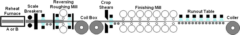
There is no single variable that can be attributed to scale formation, so to be able to determine variables that are significant in scale formation at the hot mill, it is important to identify all the process variables through a detailed description of the hot mill process. A schematic view of this process is shown in Fig. 1. The temperature is the most important variable for scale formation as scale increases exponentially with time at high temperatures. The most critical area of the hot mill for scale formation is between the crop shears and the finishing mill. To be able to understand the impact of this critical area on scale formation, multiple temperature readings are made for each coil including an average value, maximum and minimum temperatures across the coil and the temperatures at the front and back of the coil. The chemistry of the steel substrate also has a strong influence on the type of scale that will form in the hot mill. The chemistry of the coil is measured on a cast basis at the basic oxygen steelmaking plant.

Figure 1

Port Talbot hot mill layout

As illustrated in Fig. 1, steel with a specific alloying composition is reheated in furnaces and passes through scale breakers. Let variables x₁ to x₁₂ be the amounts of various alloying elements, by wt-, contained within this steel. At the edging and rougher mills, the gauge of the incoming slab is reduced from 250 to 35 mm (and the processed steel at this stage is often termed the transfer bar). The hot mill at the Tata works in Port Talbot (UK) has a reversing rougher, hence several passes are necessary to achieve the required transfer bar thickness. The transfer bar is then held at the coil box to increase the heat of the bar before entering the finishing mill. The length of time that the transfer bar can be held at the coil box depends on the temperature that the transfer bar is required to be at entry to the finishing mill. The temperature of the transfer bar is dependent on the dimensions of the bar, the processing history (after the reheat furnace) and the time that the transfer bar takes in completing the process. Let variables x₁₃ to x₁₅ be various temperatures (as described above) recorded at the rougher mill.

The crop shear temperature is the temperature just before the transfer bar enters the finishing mill. The crop shear temperature is likely to be of vital importance for predicting scale formation because tertiary scale is formed during the early stages of the finishing mill. Let variables x₁₆ to x₁₈ be various temperatures recorded at the crop shear stage of the process. On entry into the finishing mill, the slab encounters the descalers and the purpose of these is to remove scale on the surface of the coil during the hot rolling process.9 To remove more adherent scale, higher impact pressures are used, which has the negative effect of reducing more heat from the slab. Understanding the impact of the descaler is an important section of understanding the influence of scale removal, but will not be considered in this paper. Owing to the statistical methods being used, the influence of the descaler will be difficult to extract without prior knowledge of the influence of temperature and chemistry.

The purpose of the finishing mill is to further reduce the gauge to 1·4–18·0 mm. The finishing mill also controls the shape and temperature of the strip that in turn controls the metallurgical properties achieved by the strip. Let variables x₁₉ to x₂₁ be the various temperatures recorded at the finishing mill. The phase transformation occurs on the ROT and the cooling is controlled with a water cooling system. The temperature control of the ROT is vital in controlling the austenitic phase transformation. The temperature, cooling rate and cooling path will affect the microstructure present, which in turn will control the mechanical properties of the steel. Let variable x₂₂ be the temperature recorded at the ROT. However, the ROT temperature control sprays are not effective at removing scale, because the scale is formed at the entrance to the finishing mill.

Data collection

The Parsytec inspection system is a camera operated system that detects defects on the surface of the coil. The detection of defects is achieved by the identification of all non-homogeneous sections of the strip. When the affected sections are detected, then the Parsytec software classifies the detected sections into features. These features are compared to the online defect catalogue and then the best result is what the detected section is labelled as the appropriate defect. It is possible for defects to be misclassified or not classified. This can occur because the environment around the cameras has a lot of potential contamination including:

water from the descaler and cooling sprays at the finishing mill

overlapping defects

iii

substrate appearance. Every steel composition will have a different surface appearance under the Parsytec cameras that makes detection rates variable.

The Parsytec system monitors the top and the bottom of the strip, but they are located in different locations on the mill. The top surface monitor is located at the start of the ROT, while the bottom surface monitor is located at the end of the ROT just before coiling. Owing to the fact that under high coiling temperatures scale can continue growing on the ROT and that due to water and other contamination after leaving the finishing mill it was determined that the bottom surface monitor's scale count would give more reliable results.

The dataset is constructed using data associated with coils from Tata Steel Europe's Port Talbot Hot Mill, collected using the Parsytec system described above. Each of the coils in the dataset is intended for a high surface quality tinplate application, so scale levels must be low. To minimise the effect of different heating/cooling cycles, only a single gauge of 2·1 mm is investigated in this paper. Coil data were collected between September 2009 and March 2010 for all the process variables described above and Table 1 gives some descriptive statistics for this sample of data, together with the full name of each process variable and its short hand descriptor x_j. The sample size was n = 1577.

Table 1

Process variables and their sample means and standard deviations

Process variable*	x _j	Mean	Standard deviation
carbon	x ₁	0·069	0·0042
manganese	x ₂	0·485	0·0226
phosphorus	x ₃	0·014	0·0031
sulphur	x ₄	0·014	0·0030
silicon	x ₅	0·005	0·0032
copper	x ₆	0·016	0·0059
nickel	x ₇	0·010	0·0030
chrome	x ₈	0·018	0·0040
aluminium	x ₉	0·034	0·0047
tin	x ₁₀	0·003	0·0018
nitrogen	x ₁₁	0·012	0·0009
solAl	x ₁₂	0·031	0·0043
Maximum RM temperature/°C	x ₁₃	1121·75	17·87
Minimum RM temperature/°C	x ₁₄	918·34	11·97
Average RM temperature/°C	x ₁₅	1099·43	16·18
Maximum CS temperature/°C	x ₁₆	1099·88	19·89
Minimum CS temperature/°C	x ₁₇	951·69	48·59
Average CS temperature/°C	x ₁₈	1069·55	20·80
Maximum FM temperature/°C	x ₁₉	907·16	7·18
Minimum FM temperature/°C	x ₂₀	829·87	28·96
Average FM temperature/°C	x ₂₁	881·05	5·75
ROT temperature/°C	x ₂₂	731·35	25·13
Scale count indicator	y†	0·327	0·469

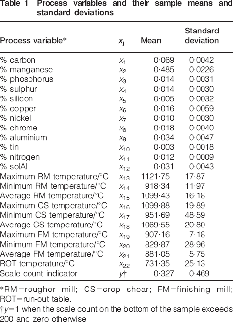
*RM = rougher mill; CS = crop shear; FM = finishing mill; ROT = run-out table.

†y = 1 when the scale count on the bottom of the sample exceeds 200 and zero otherwise.

The dependent variable y is a binary classification based on the scale count from the Parsytec system. The dependent variable takes on a value of unity when the scale count on the bottom of the table exceeds 200 and zero otherwise. The cut of 200 was chosen for two main reasons. The first reason was that lower scale counts than this are unlikely to be a problem for further processing but as the scale count increases above 200, it becomes more difficult to determine if the scale will cause a problem for further processing without understanding how adherent the scale is. The second reason is that a split of 200 makes the population of bottom surface affected coils represent >30 of the dataset which makes it easier to be confident about the output of the models, i.e. it creates a more balanced dataset from which to apply non-linear PLS to.

Partial least squares generalised linear regression algorithm

The PLS regression method in its basic form applies to one single response variable y and is non-iterative. It is particularly useful when the x_j variables are closely correlated with each other. Marx10 proposed a generalisation of the PLS algorithm to generalised linear models (see McCullagh and Nelder11 for an excellent account of generalised linear models). This approach is very useful because the binary logit model can be given a generalised linear regression representation. Marx10 used the fact that, in the context of the exponential family, maximum likelihood estimates are obtained by an iterative weighted least squares procedure. His approach consisted of replacing the iterative weighted least squares step by a sequence of PLS regressions.

Generalised linear model

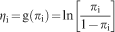
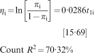
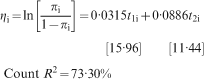
Suppose that a sample of i = 1 to n specimens have been scanned for scale formation on the ROT of the hot mill. Then let y_i be the binary response that equals unity when significant scale (defined as a scale count for the Parsytec system in excess of 200) is detected on the bottom of the tested specimen and zero otherwise. Next let π_i be the probability of significant scale formation and also let x_1i, …., x_pi be all the explanatory or process variables described in the previous section. Finally, let g(π_i) be the link function. Then the generalised linear regression model has the following form (1a) where (1b) and where there are p process variables. The model parameters β_j can be estimated using the iterative weighted least squares procedure put forward by McCullagh and Nelder.11 This procedure involves the creation of an adjusted dependent variable z_i with components (2a) If then, the following (n×n) diagonal matrix of weights is calculated (2b) then the following standard weighted least squares formula can be used to estimate the β_j (2c) where X is a (n×p) matrix of the process variables x_{1, …}, x_p such that the first column of X contains the n values for x₁ and the last column of X contains the n values for x_p. X^T is the transpose of X and Z is an (n×1) vector containing the n values for z_i as defined by equation (2a). β is of course a (p×1) vector containing the estimates for β₁ to β_j. This has to be an iterative solution where initial guesses for β₁ to β_j are inserted into equation (1) to enable values for z_i and W to be calculated from equation (2a) and (2b). Equation (2c) then gives revised or improved estimates for β₁ to β_j. These revised values are then used to recalculate values for z_i and W from which further revised estimates for β₁ to β_j are obtained. This iterative process continues until the changes in all the β_j values are very small.

Partial least squares within generalised linear model

Within this setting, the following PLS generalised linear regression algorithm can be stated. This algorithm follows closely that given by Bastien and Tenenhaus.12 Let 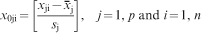X₀ be the matrix containing the n values for the standardised input variables x₀₁, …, x_0p (3) where is the sample average for the n values on variable x_j and s_j is the corresponding sample standard deviation (the last two columns of Table 1 show these two statistics for each process variable). Then, the first column of X₀ contains the n values for x₀₁, and the last column of X₀ contains the n values for x_0p. Within this setting, the PLS components can be derived as follows.

Determination of first PLS component t_1i

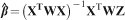
for each j = 1 to p, compute the regression coefficient β_1j of x_0j in the generalised linear regression model given by equation (1a) and (1b) of y_i on x_0ji using the iteratively weighted least squares procedure described above

for each j = 1 to p, compute the standard error se_1j, of the regression coefficient β_1j of x_0j in the generalised linear regression model given by equation (1a) and (1b) of y_i on x_0ji using the iteratively weighted least squares procedure described above. Then compute the Student t statistic v_1j = β_1j/se_1j

iii

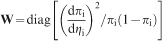
form the vector β₁ = (β₁₁, …, β_1p)^T, and a (p×p) diagonal matrix of weights v₁ = diag(v_1j) and the (p×1) vector v₁β₁

compute the vector t₁ = X₀ v₁β₁. t₁ is a vector made up of the n values of t_1i and constitutes the first PLS component.

This PLS component is essentially a weighted average of the p predictors of y_i, namely a weighted average of the β_1jix_0ji series. A cruder but simpler version of this is to simply delete from β₁ those coefficients that are found to be statistically insignificant at the 1 significance level using the Student t test, and of course the corresponding process variable from X₀,when forming the vector t₁. (The justification being that v_1j will be small if the Student t value for β_1j = 0 is less than the 1 significance level).

Determination of second PLS component t_2i

compute the residuals from the set of linear regressions of each column of X₀ on t₁ and store these residuals in the matrix X₁. (For example, x_1j would be the first column in X₁ and would contain the n residuals derived from the linear regression of x_01i on the t_1i

for each j = 1 to p, compute the regression coefficient β_2j of x_1j in the generalised linear regression model of y_i on t_1i and x_1ji using the iteratively weighted least squares procedure described above

iii

for each j = 1 to p, compute the standard error se_2j, of the regression coefficient β_2j of x_1j in the generalised linear regression model of equation (1a) and (1b) of y_i on x_1ji using the iteratively weighted least squares procedure described above. Then compute the Student t statistic v_2j = β_2j/se_2j

form the vector β₂ = (β₂₁, …, β_2p)^T, a (p×p) diagonal matrix of weights v₂ = diag(v_2j) and the (p×1) vector v₂β₂

compute the vector t₂ = X₁ v₂β₂. t₂ is a vector made up of the n values of t_2i. It is essentially a weighted average of the p predictors of y_i given in step (i). Again a cruder but simpler version of this is to simply delete from β₂ those coefficients that are found to be statistically insignificant at the 1 significance level using the standard Student t test, and of course the corresponding transformed process variable from X₁, when forming the vector t₂.

Determination of other PLS components

This procedure is iterated for the other PLS components t_hi. At each step the generalised linear regression of y_i on components t_1i, …, t_hi is carried out. The procedure is stopped, and the component t_m+1i is not included in the model if that component is not statistically significant at the 5 significance level using the standard Student t test. The final regression equation is obtained by expressing the generalised linear regression of y_i on t_1i, …, t_mi and this can also be written as a function of the original variables by making use of the standardisation procedure given in equation (3) and the means and standard deviations are given in Table 1. In the case of ordinary multiple regression, this algorithm gives the usual PLS regression when there is no missing data.

Results

Partial least squares components and PLS logit model

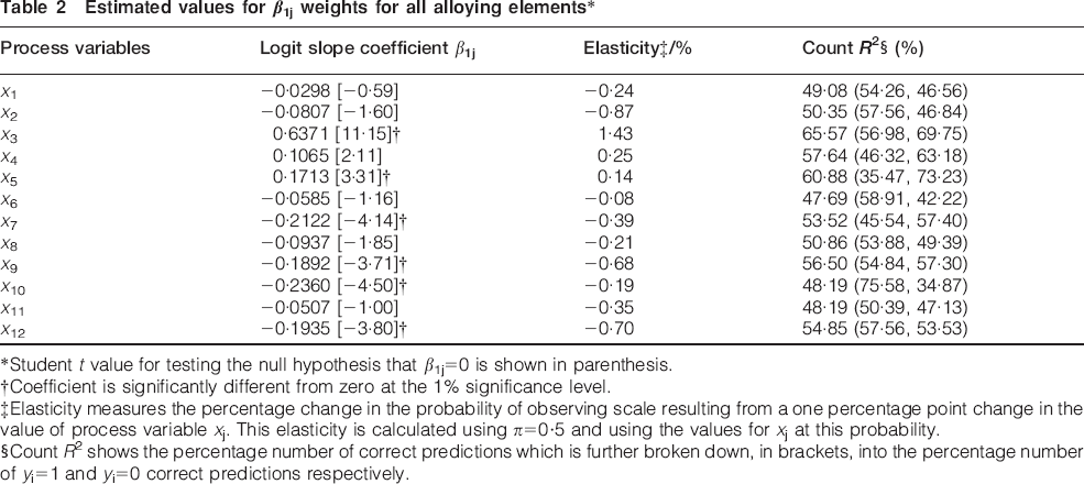
Table 2 shows the estimated values for the β_1j weights of the first PLS components associated with all the different alloying elements. (see Table 1 for a description of the shorthand used for each of the process variables listed in Tables 2 and 3)

Table 2

Estimated values for β_1j weights for all alloying elements*

Process variables	Logit slope coefficient β_1j	Elasticity‡/	Count R²§ ()
x ₁	−0·0298 [−0·59]	−0·24	49·08 (54·26, 46·56)
x ₂	−0·0807 [−1·60]	−0·87	50·35 (57·56, 46·84)
x ₃	0·6371 [11·15]†	1·43	65·57 (56·98, 69·75)
x ₄	0·1065 [2·11]	0·25	57·64 (46·32, 63·18)
x ₅	0·1713 [3·31]†	0·14	60·88 (35·47, 73·23)
x ₆	−0·0585 [−1·16]	−0·08	47·69 (58·91, 42·22)
x ₇	−0·2122 [−4·14]†	−0·39	53·52 (45·54, 57·40)
x ₈	−0·0937 [−1·85]	−0·21	50·86 (53·88, 49·39)
x ₉	−0·1892 [−3·71]†	−0·68	56·50 (54·84, 57·30)
x ₁₀	−0·2360 [−4·50]†	−0·19	48·19 (75·58, 34·87)
x ₁₁	−0·0507 [−1·00]	−0·35	48·19 (50·39, 47·13)
x ₁₂	−0·1935 [−3·80]†	−0·70	54·85 (57·56, 53·53)

*Student t value for testing the null hypothesis that β_1j = 0 is shown in parenthesis.

†Coefficient is significantly different from zero at the 1 significance level.

‡Elasticity measures the percentage change in the probability of observing scale resulting from a one percentage point change in the value of process variable x_j. This elasticity is calculated using π = 0·5 and using the values for x_j at this probability.

§Count R² shows the percentage number of correct predictions which is further broken down, in brackets, into the percentage number of y_i = 1 and y_i = 0 correct predictions respectively.

Table 3

Estimated values for β_1j weights for various temperatures*

Process variables	Logit slope coefficient β_1j	Elasticity‡/	Count R²§ ()
x ₁₃	0·7274 [11·84]†	22·83	63·28 (72·67, 58·72)
x ₁₄	0·0299 [0·59]	1·18	55·49 (38·57, 63·72)
x ₁₅	0·8002 [12·80]†	27·18	64·24 (72·67, 60·14)
x ₁₆	0·7175 [11·74]†	19·84	64·55 (71·51, 61·17)
x ₁₇	0·2140 [3·98]†	2·10	53·77 (68·99, 46·37)
x ₁₈	0·7465 [10·76]†	19·19	64·23 (75·00, 59·00)
x ₁₉	0·5033 [8·85]†	31·78	61·00 (55·81, 63·52)
x ₂₀	0·2205 [4·29]†	3·16	49·78 (71·51, 39·21)
x ₂₁	0·5851 [11·44]†	44·85	65·38 (66·67, 64·75)
x ₂₂	−0·2130 [−3·88]†	−3·10	54·60 (41·28, 61·07)

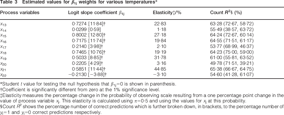
*Student t value for testing the null hypothesis that β_1j = 0 is shown in parenthesis.

†Coefficient is significantly different from zero at the 1 significance level.

§Count R² shows the percentage number of correct predictions which is further broken down, in brackets, to the percentage number of y_i = 1 and y_i = 0 correct predictions respectively.

Only the slope coefficients in front of the elements P, Si, Ni, Mo, Al, S and solAl are statistically significant at the 1 significance level. Of these elements, increases in the amount of P and Si lead to an increase in the probability of scale formation, while increases in the other elements had a negative impact. Further, of these statistically significant elements, only P (and possible Al and solAl) seems to have predictive power for both y_i = 0 and y_i = 1 (as measured by count R²) above that given by purely random predictions. The estimated elasticities are however quite small (especially when compared to the temperature variables in Table 3), with for example a 1 increase in phosphorous content bringing forth a 1·43 increase in the chances of significant scale forming (when this probability is already at 0·5).

Table 3 shows the estimated values for the β_1j weights of the first PLS components associated with all the different temperatures. Only the minimum rougher mill temperature appears to be statistically insignificant at the 1 significance level and all but the average ROT temperature has the expected sign – with increases in temperature bringing forth an increase in the probability of significant scale forming. The average finishing mill temperature appears to have the biggest effect, with a 1 increase in this temperature bringing forth a 44·85 increase in the chances of significant scale forming (when this probability is already at 0·5). In terms of the count R² values, the average rougher and finishing mill temperatures have the best predictive capabilities for both y_i = 1 and y_i = 0.

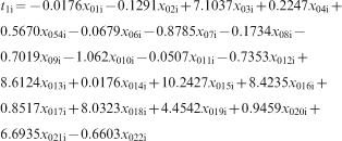
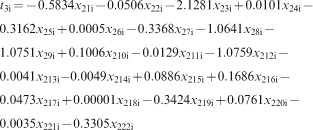
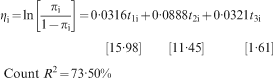
Using the algorithm described above and the values shown in Tables 2 and 3, the first PLS component, written out in terms of the standardised values for the process variables, can be computed as follows (4a) The first PLS component, written out in terms of the process variables in their original units, can also be computed as follows (4b) Then when t_1i is used instead of all the process variables, the following PLS logit model is obtained using iteratively weighted least squares (4c) The Student t value given in parenthesis shows that this PLS component is significantly different from zero at the 1 significance level, so it is an important predictor variable of significant scale formation. This PLS model predicts the formation of scale or lack of scale with just over 70 accuracy, which given the very large variability in the data is a good outcome. Further, the count R² associated with y_i = 1 suggests that the model can predict the processing conditions that lead to excessive scale with 80·43 accuracy (but the count R² associated with y_i = 0 is lower at 65·41).

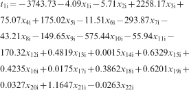
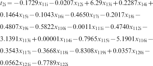
Using the above algorithm, the next PLS component using the standardised process variables was identified as (5a) or in terms of the process variables in their original units, this can be rewritten as (5b) The extended PLS logit model with this extra component in is then estimated by iterative weighted least squares to be (5c) The Student t values given in parenthesis shows that both these PLS components are significantly different from zero at the 1 significance level, so they are important predictor variables of scale formation. This PLS model predicts the formation of scale or lack of scale with just over 73 accuracy and so the addition of the second PLS adds an additional 3 to overall predictive accuracy of the previous model given by equation (4c). Further, the count R² associated with y_i = 1 suggests that the model can predict the processing conditions that lead to excessive scale formation with 84·69 accuracy (but the count R² associated with y_i = 0 is lower at 67·77).

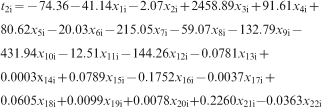
Using the above algorithm, the third PLS component was identified as (6a) with the extended PLS logit model (6b) The Student t values given in parenthesis shows that the first two PLS components are significantly different from zero at the 1 significance level, but the third component is only statistically significant at the 10 significance level. Further, this PLS logit model only has an additional 0·2 overall predictive accuracy compared to that given by equation (5c). Taken together, these two facts suggest that the PLS logit model with just two components is a valid parsimonious model, i.e. the model given by equation (5c).

Analysis and interpretation

Figure 2 plots the scale indicator variable y_i against the PLS component t_1i. Also shown are the predicted probabilities of scale formation given by the above parsimonious PLS logit model. These predictions are consistent with the spread of y_i values shown on this figure. When the second PLS component is zero, scale formation becomes more likely than not when the first principle component exceeds zero in value. At this value for t_1i, a change in t_2i has a big impact on the probability of scale formation.

Figure 2

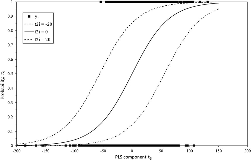
Predicted probabilities of scale formation as function of PLS components

Figure 3 plots the first two PLS components against each other with the data points shaded or unshaded depending upon whether the scale indicator variable is zero or unity. It is clear from this figure that samples with significant scale formation tend to correspond to those with higher t_1i values – more specifically with positive t_1i values. Variations in the values for t_2i are far less indicative of whether scale has formed or not. These positive t_1i values can be traced back to the specific operating conditions. Clearly, many different conditions can be identified to achieve a required rate of scale formation, but Fig. 4 and Table 4 give an indication of what can be achieved.

Figure 3

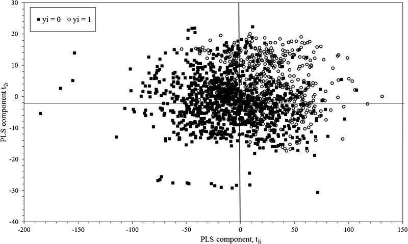
Cross plot of PLS components

Figure 4

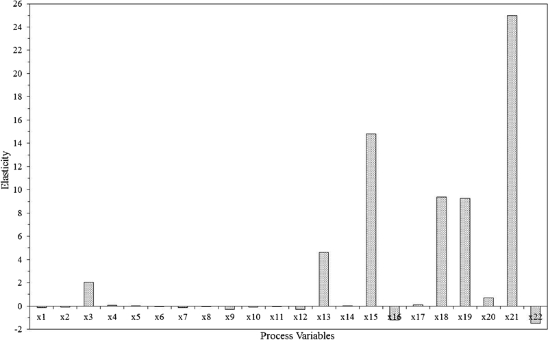
Calculated elasticities for each process variable

Table 4

Examples of using PLS logit model for process control

Variable/probability	x₃/	x₁₃/°C	x₁₅/°C	x₁₈/°C	x₁₉/°C	x₂₁/°C
0·1	0·0065	855·8	1017·8	944·20	799·5	842·3
0·2	0·0093	953·9	1047·9	990·5	839·2	856·6
0·3	0·0112	1019·2	1067·9	1021·2	907·2	866·1
Sample averages	0·0141	1121·7	1099·4	1069·5	907·2	881·0

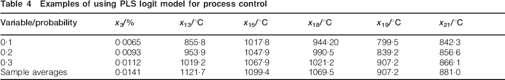
Figure 4 shows the elasticities associated with each process variable as calculated around the mean values for each process variable shown in Table 1. These elasticities give the percentage change in the probability of scale formation following a 1 change in that process variable from its mean value. It can be seen from this figure that the most important process variable appears to be the average finishing mill temperature. When this temperature is increased by 1 from its mean of 881°C (i.e. from 881 to 890°C), while keeping all the other process variables at their mean values shown in Table 1, the chance of significant scale forming as a result of this change, increased by 25, i.e. from 0·5 to 0·63. The next most important variables appear to be the average rougher mill temperature with elasticity of just under 15. In importance, this is closely followed by the average crop shear temperature and the maximum finishing mill temperature whose elasticitiess are both around 10. The only alloying element with elasticity above 2 is phosphorous. With an elasticity of 2·04, when this element is increased by 1 from its mean of 0·014 (i.e. from 0·014 to 0·01414), while keeping all the other process variables at their mean values shown in Table 1, the chance of significant scale forming as a result is this change, increased by 2·04, i.e. from 0·5 to 0·51. This is clearly a much smaller effect than that associated with the above mentioned temperature variables.

Next, Table 4 shows what the process variables with the largest elasticities should be set at so as to achieve a required low probability of scale formation when all the other process variables are set at their average values shown in Table 1. The low probabilities looked at in this table are 0·3 down to 0·1. Looking for example at the finishing mill temperature (x₂₁), to reduce the probability of significant scale forming from 0·5 (when all process variables are set at the average values shown in Table 1) to 0·1, this temperature must be set as low as 842°C (compared to the sample average value of 881°C). The same low probability of scale formation can be achieved by lowering the phosphorous content to 0·0065 (from the sample average of 0·0141) while holding all the other process variables at the sample average values shown in Table 1.

A final insight into the estimated PLS logit model can be obtained using cumulative frequency plots. This cumulative frequency plot is constructed by sorting the sample dataset, from lowest to highest, by the variable of interest and counting how many observations there are at or below various values for that variable of interest. This frequency count can then be plotted alongside the frequency count implied by the probabilities predicted from equation (5c). Figure 5 shows the cumulative frequency plot for the average roughing mill temperature. It can be seen that the observed and predicted values match quite well. The model correctly predicts when scale starts to become an issue (around 1080°C) and follows the observed frequency count until about 1120°C.

Figure 5

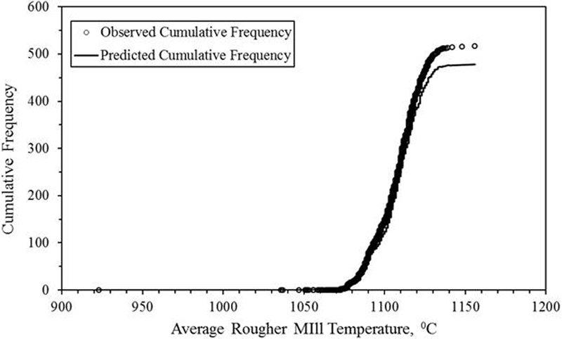
Cumulative frequency plot for average rougher mill temperature

Figure 6 shows the cumulative frequency plot for the average crop shear temperature. It can be seen that the observed and predicted values match less well in comparison to the other temperature variables. The predicted results overpredict when scale starts to become an issue (1070°C instead of ∼1060°C) and follows the observed line until ∼1090°C.

Figure 6

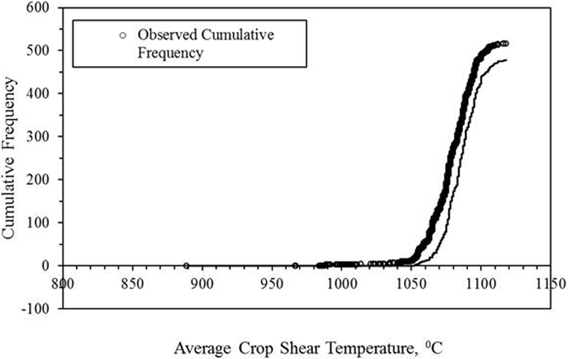
Cumulative frequency plot for average crop shear temperature

Conclusions

Using a non-linear PLS logit model, it was found that there exists only two linear PLS components that were important or statistically significant in determining scale formation in this dataset obtained from the Hot Mill at Tata Steel Port Talbot. The estimated model was capable of correctly predicting, when y_i = 1 (i.e. when significant scale formation had occurred), 85 of the time. The good predictive capability was also confirmed by the cumulative frequency plots, where it was observed that the predictions from the model with respect to those temperatures with a high elasticity corresponded well with the observed values. This was especially true for the temperature at which scale is first observed to occur.

The chances of scale forming also appeared to increase with increasing values of the first PLS component. This trend was then translated into suggested best practice operating conditions. For example, if the finishing mill temperature was set at 842°C, with all other process variables set at the average values shown in Table 1, the model predicted that the chances of significant scale forming can be kept at low as 10. The elasticities associated with the non-linear PLS logit model also showed that the main determinants of scale formation were the various temperatures. The elasticities derived from the model showed that the minimum temperatures have significantly less predictive power than the maximum and average temperatures at the various stages of operation within the hot mill. The most important temperatures for scale formation were the average temperatures at the rougher and finishing mills, as well as the average crop shear temperature. It was also found that the only chemistry element that had a major part to play in scale formation was the amount of phosphorus present in the coil. This might be because the phosphorus could be increasing the adhesion of the scale to the coil substrate.

Footnotes

Acknowledgements

The authors are grateful for the support of Tata Strip UK, and personnel within Port Talbot Hot Mill. The authors are also grateful for the funding received from the Engineering and Physical Sciences and Research Council (EPSRC) and Tata Steel Strip Products UK.

References

Haapamaki

, Tamminen

, Roning

: ‘Data mining methods in hot steel rolling for scale defect prediction’, Proc. AIA 2005, Innsbruck, Austria, February 2005, IASTED, 453–464.

Haapamaki

, Roning

: ‘Genetic algorithms in hot steel rolling for scale defect prediction’, Eng. Technol. , 2005, 5, 1–4.

Bolt

: ‘Understanding the properties of oxide scale on hot rolled strip’, Proc. METEC Congress 03/3rd Eur. Rolling Conf. (ERC), 16–18 June, Dusseldorf, Germany, June 2003.

Taniguchi

, Yamamoto

, Megumi

, Shibata

: ‘Characteristics of scale/substrate interface area of Si-containing low-carbon steels at high temperatures’, Mater. Sci. Eng. A , 2001, A308, 250–257.

Yang

, Yang

, Lin

, Chen

, Tsai

: ‘Effects of Si and its content on the scale formation on hot-rolled steel strips’, Mater. Chem. Phys. , 2008, 112, 566–571.

Munther

, Lenard

: ‘The effect of scaling on interfacial friction in hot rolling of steels’, J. Mater. Process. Technol. , 1999, 88, 105–113.

H. Bolt: The Properties of Oxide Scales on Hot Rolled Steels: A Literature Review, Corus Research, Development & Technology, Ijmuiden Technology Centre, 2000.

Sun

, Tieu

, Jiang

, Zhu

, Lu

: ‘Oxide scales growth of low-carbon steel at high temperatures’, J. Mater. Process. Technol. , 2004, 155–156, 1300–1306.

Silk

: ‘The practical aspects of hydraulic de-scaling’, Steel Times Int. , Oct. 2001, 38–44.

10.

Marx

: ‘Iteratively reweighted partial least squares estimation for generalized linear regression’, Technometrics , 1996, 38, (4), 374–381.

11.

McCullagh

, Nelder

: ‘Generalised linear models’, 2nd edn; 1989, London, Chapman & Hall.

12.

Bastien

, Tenenhaus

: ‘PLS generalized linear regression: application to the analysis of life time data’, Comput. Stat. Data Anal. , 2005, 48, (1), 17–46.