
Abstract
The effective mobility approach is compared with the kinetic energy approach in terms of sharp interface modeling and phase-field modelling of non-equilibrium solute diffusion upon rapid solidification of binary alloys. The two approaches are equivalent for modelling of long range solute diffusion in bulk phases, but only the effective mobility approach can introduce the non-equilibrium solute diffusion effect to short range solute diffusion at a sharp interface or within a diffuse interface. Addition of the kinetic energy terms results in an unreasonable non-bilinear expression of the flux and thermodynamic driving force in the free energy production of interface migration or phase field propagation, whereas the effective mobility approach allows the thermodynamic extremal principle workable.
Introduction
Rapid solidification is extremely interesting for both scientific and technological reasons. It is not only a good technique for preparing materials of potential novel properties but also a good subject for studying non-equilibrium phenomena. 1 Upon rapid solidification, several irreversible dissipative processes occur concurrently, e.g. solute diffusion in bulk phases, trans-interface diffusion (or solute redistribution) and interface migration at the growing sharp interface.2,3 The first and second dissipative processes belong respectively to long and short range solute diffusion.4,5
The solute diffusion velocity in bulk liquid  (of order 0.1–10 m s− 1)
6
determines how fast a solute atom can travel in liquid.
7
The interfacial solute diffusion velocity
(of order 0.1–10 m s− 1)
6
determines how fast a solute atom can travel in liquid.
7
The interfacial solute diffusion velocity  is comparable with but is smaller than
  .
8
[The diffusion velocity is a characteristic velocity above which solute diffusion cannot occur any more. It can be defined as VD = (D/τ)1/2 with D the diffusion coefficient and τ the relaxation time of solute diffusion to its equilibrium state.] The maximal interface velocity Vo is equal to the speed of sound if interface migration is collision limited.
1
Practically, the measured interface velocity V, which approaches 10–100 m s− 1,
1
can be comparable with or even larger than
.
8
[The diffusion velocity is a characteristic velocity above which solute diffusion cannot occur any more. It can be defined as VD = (D/τ)1/2 with D the diffusion coefficient and τ the relaxation time of solute diffusion to its equilibrium state.] The maximal interface velocity Vo is equal to the speed of sound if interface migration is collision limited.
1
Practically, the measured interface velocity V, which approaches 10–100 m s− 1,
1
can be comparable with or even larger than  . In this case, solute diffusion is not only determined by its instantaneous concentration gradient but also relevant to its local evolution history, i.e. non-equilibrium solute diffusion (NESD).
9
Modelling of NESD upon rapid solidification, therefore, becomes quite important for the understanding of non-equilibrium phenomena.3,6–24 Two different recipes have been proposed, i.e. the kinetic energy approach
13
and the effective mobility approach.
23
. In this case, solute diffusion is not only determined by its instantaneous concentration gradient but also relevant to its local evolution history, i.e. non-equilibrium solute diffusion (NESD).
9
Modelling of NESD upon rapid solidification, therefore, becomes quite important for the understanding of non-equilibrium phenomena.3,6–24 Two different recipes have been proposed, i.e. the kinetic energy approach
13
and the effective mobility approach.
23
Kinetic energy approach
In order to describe NESD by phase field modelling, the ‘slow’ variable in the classical irreversible thermodynamics {c} and the ‘fast’ variable in the extended irreversible thermodynamics,
9
 can be integrated to form a general space of variables
  .
13
This is equivalent to add a so called kinetic energy term
.
13
This is equivalent to add a so called kinetic energy term  to the classical free energy density. Here, c is the overall solute molar fraction,
  is the overall solute flux and
  is the kinetic coefficient that is independent of
  .
13
As a result, a second derivation of c with respect to time is added to the classical Cahn–Hilliard equation.
25
To show more about the kinetic energy approach
13
.
13
As a result, a second derivation of c with respect to time is added to the classical Cahn–Hilliard equation.
25
To show more about the kinetic energy approach
13
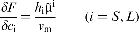
 from the kinetic energy term
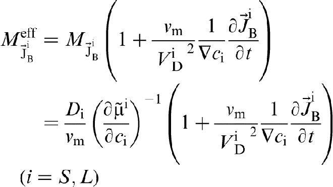
  to the thermodynamic driving force of solute diffusion if its mobility
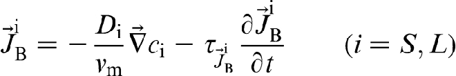
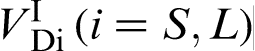
  is taken as the independent variable on the NESD effect. Here, ‘S’ and ‘L’ denote respectively the value in solid and liquid, Di is the solute diffusion coefficient, vm the atomic volume is assumed to be the same for solvent A and solute B, ci is the solute molar fraction,
  is the relaxation time of
  ,
,  is the solute diffusion potential and
 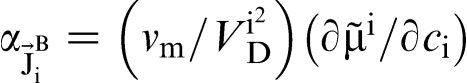 is a kinetic parameter independent on
  . The kinetic energy
13
suggests that the NESD effect changes the thermodynamic state in the case of a prescribed kinetic mobility. This approach was widely used to propose the sharp interface model,3,16 phase field model13,17,18,21 and phase field crystal models.7,19,20
. The kinetic energy
13
suggests that the NESD effect changes the thermodynamic state in the case of a prescribed kinetic mobility. This approach was widely used to propose the sharp interface model,3,16 phase field model13,17,18,21 and phase field crystal models.7,19,20
Effective mobility approach
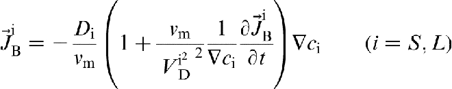
Noting that the Maxwell–Cattaneo equation
9
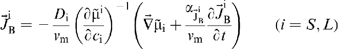
equation (1) can also be reformatted as
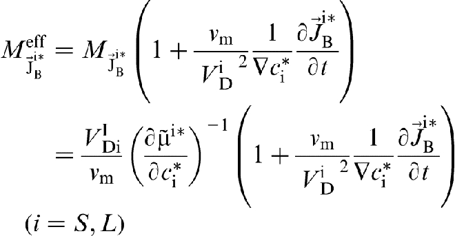
 was assumed to be the independent variable on the NESD effect. In this case, the effective mobility of solute diffusion changes from
 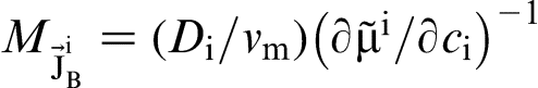 to an effective one
 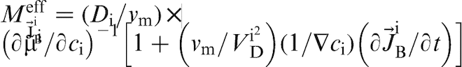 with
with 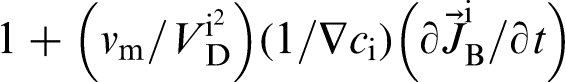 as a dimensionless effective mobility term (see equation (3). The effective mobility approach
23
in the case of a prescribed thermodynamic state changes the kinetic mobility.
as a dimensionless effective mobility term (see equation (3). The effective mobility approach
23
in the case of a prescribed thermodynamic state changes the kinetic mobility.
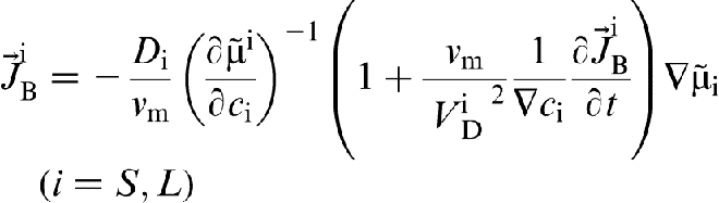
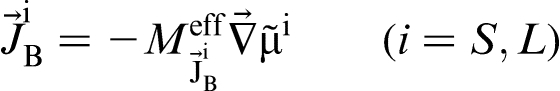
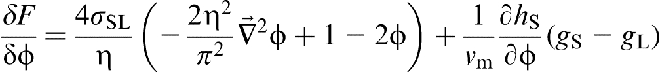
If the driving force for solute diffusion is taken as the gradient of solute molar fraction  , equation (3) reduces to
 can then be defined by comparing equation (4) with the classical Fick's law
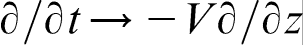
 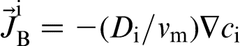 . In the case of one-dimensional steady state growth, a standard coordinate transformation
  with V as a constant interface velocity reduces
  to
to
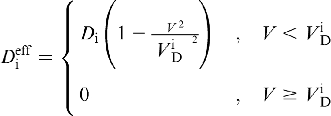
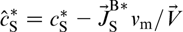
 , the classical theory can be extended directly to the case of NESD. For example, if
  is defined approximately as
  , with η the interface thickness, the solute trapping model of Aziz26,27 can be modified as8,10
 in equation (6) in which
  as
as  , complete solute trapping
  happens abruptly at a finite interface velocity
  . This solute trapping model with the NESD effect has been verified by experiments8,10–12 and atomistic simulations.
24
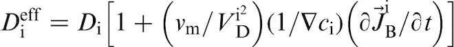
As compared with the effective diffusion coefficient of Sobolev,
10
both the kinetic energy approach
13
and the effective mobility approach
23
are applicable to the case of non-steady state growth.
. This solute trapping model with the NESD effect has been verified by experiments8,10–12 and atomistic simulations.
24
As compared with the effective diffusion coefficient of Sobolev,
10
both the kinetic energy approach
13
and the effective mobility approach
23
are applicable to the case of non-steady state growth.
This work aims to carry out a comparative study between the kinetic energy approach 13 and the effective mobility approach 23 in terms of examples for sharp interface modelling and phase field modelling of NESD upon rapid solidification of binary alloys. It will be shown that the two approaches are equivalent for modelling of long range solute diffusion in bulk phases, but only the effective mobility approach 23 can introduce the NESD effect to short range solute diffusion (or solute redistribution) at a sharp interface or within a diffuse interface. The effective mobility approach 23 therefore should be dominant in modelling of NESD upon rapid solidification.
Sharp interface modelling of rapid solidification of binary alloys
Total free energy and its change rate
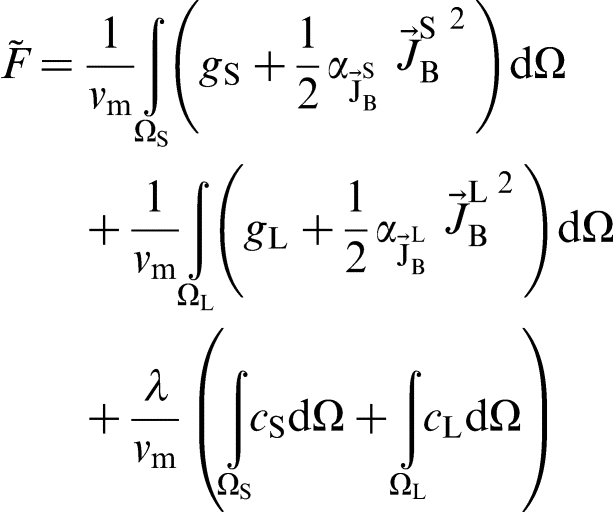
In the case of a sharp interface, a generalised total free energy  in the entire volume
  (see Fig. 1) is given by
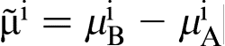
 with
with  (i = S, L; j = A, B) the chemical potential, and the associated Lagrange multiplier λ is included to ensure the global solute conservation in a closed system (i.e.
  ). The introduction of the generalised total free energy
  by combining of the total free energy F with
 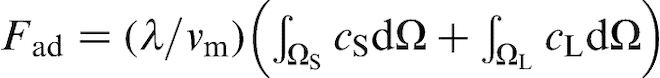 that is not a real contribution to total free energy is helpful to describe the additional constraints thermodynamically consistently as will be shown in what follows.
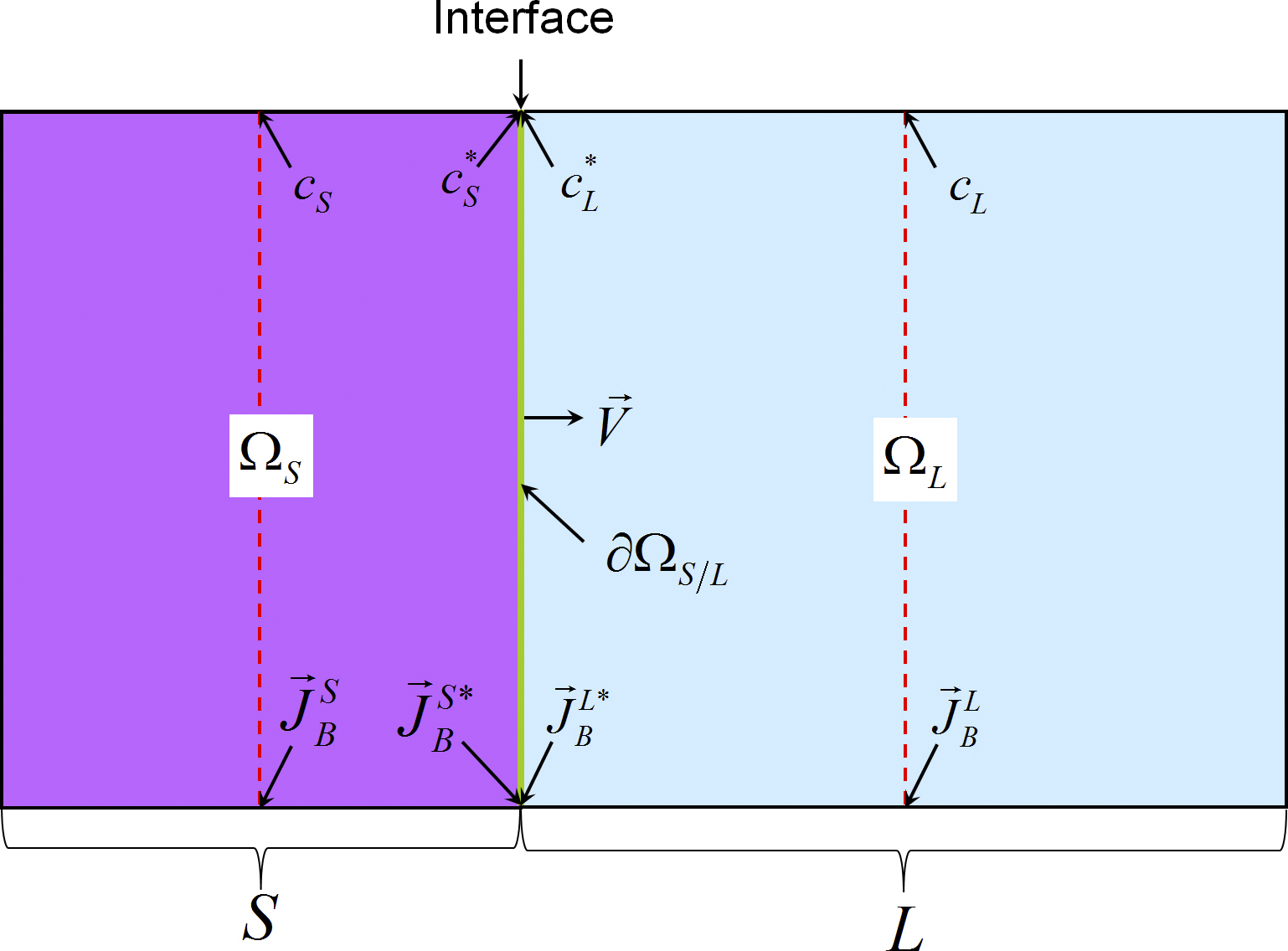
Schematic diagram for isothermal rapid solidification of binary alloys; solute jump happens at sharp interface
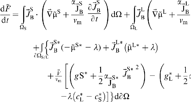
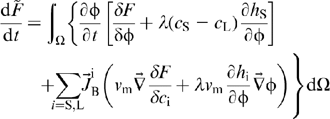
Differentiating equation (7) with respect to time by the help of the transport theorem
28
and using the Gibbs–Duhem relation  (i = S, L) and the solute conservation law
 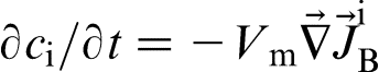 , the change rate of total free energy is obtained as
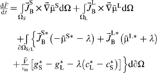
 and
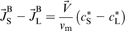
and 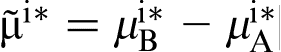 (i = S, L) are respectively the solute diffusion potentials in bulk phases and at the interface. The change rate of total free energy equation (8) is a bilinear expression in the fluxes and thermodynamic driving forces. The first and second terms on the right hand side of equation (8) correspond to long range solute diffusion in solid and liquid whose fluxes and conjugative driving forces are
  and
and  (
( ). The third term is for the dissipative processes at the interface, i.e. short range solute diffusion in solid (liquid) whose flux and driving force are
  and
and  (
( ) and interface migration whose crystallisation flux and driving force are
 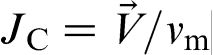 and
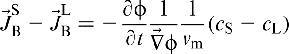
and  . The three dissipative processes are constrained by the solute balance, which can be derived from the terms with the Lagrange multiplier λ in equation (8)

 is the solute molar fraction transferred across the interface,29,30 and Δ denotes the difference between the variable in solid and liquid. The dissipations at the interface are summarised in Fig. 2.
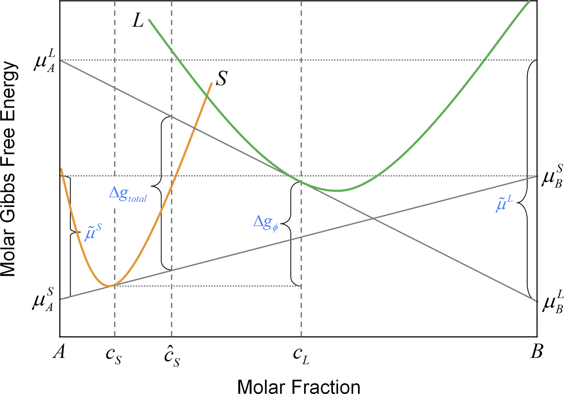
Molar Gibbs free energy diagram for isothermal solidification of binary alloys: if solute diffusion in solid is significant at sharp interface, there are three dependent dissipative processes (i.e. solute diffusion in solid and liquid at interface and interface migration with fluxes respectively as
,  and
and  ) and one additional constraint from solute balance at sharp interface (i.e. equation (9))
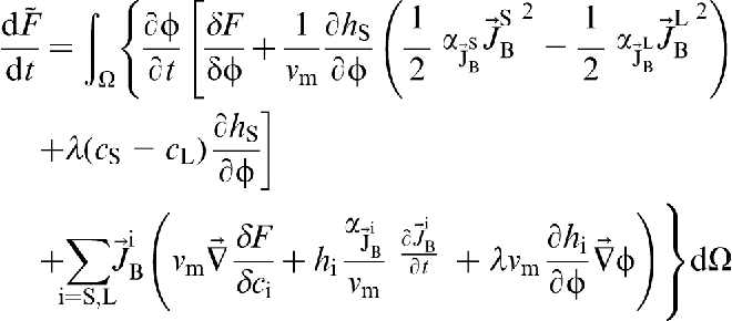
If the kinetic energy terms, i.e. (
( ), are added to the total free energy of the system, equation (7) is rewritten as
 (
( )
13
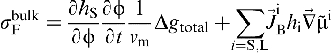
and following a similar derivation procedure as equation (8), we have
)
13
and following a similar derivation procedure as equation (8), we have
 (
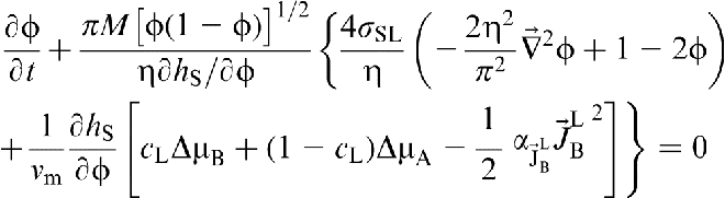
( ) from the kinetic energy; please see the first and second terms on the right hand side of equation (12). For the dissipative processes at the interface, the NESD effect is not introduced to short range solute diffusion in solid and liquid; please see the first and second terms in the brace of equation (12). The free energy production of interface migration, i.e. the third term in the brace of equation (12), however, becomes a non-bilinear expression in the flux and thermodynamic driving force.
Evolution equations
Owing to its particular advantages in modelling of non-equilibrium dissipative systems with additional constraints, the thermodynamic extremal principle (TEP)31–37 is adopted here to derive the evolution equations. For a general understanding and its extensive application to various fields of materials science, the readers are referred to a recent review of Fischer et al.
37
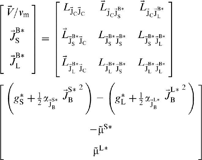
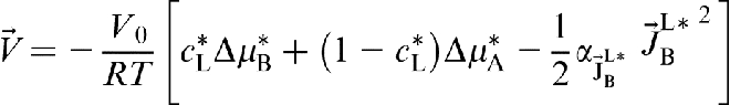
The evolution of the system according to the TEP of Svoboda et al.34–37 for the linear irreversible thermodynamics is given by
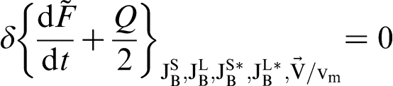
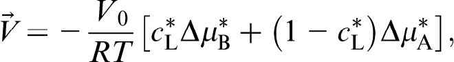
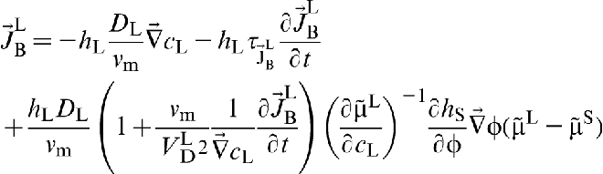
 in terms of the effective mobility approach is expressed as
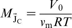
 is the interfacial solute diffusion velocity, R is the gas constant and T is the temperature.
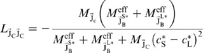
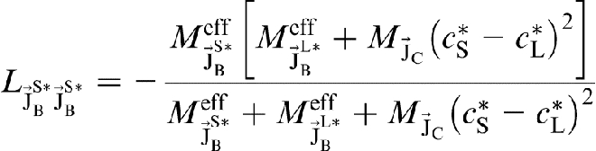
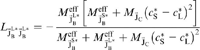
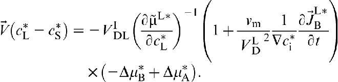
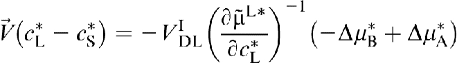
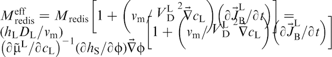
Substituting equations (8) and (14) into the extremal condition equation (13) and then eliminating the Lagrange multiplier λ by equation (9), one obtains the evolution equations for the bulk phases
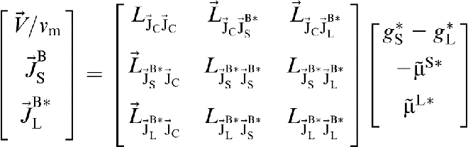
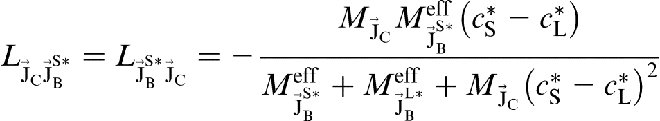
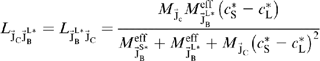
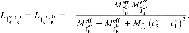
Adopting the effective mobilities ((equations (19)–(25)), by setting  and using equations (9) and (16), are rewritten as
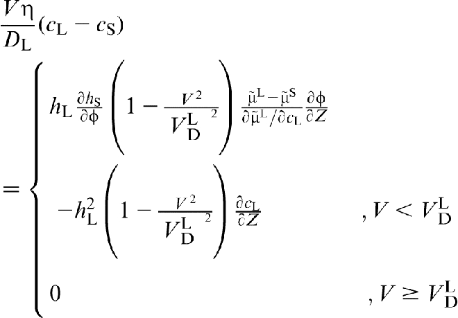
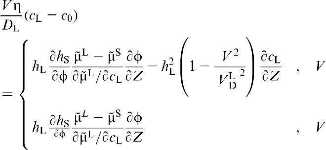
 . The two dissipative processes at the interface are summarised in Fig. 3. In the case of one-dimensional steady state growth, a standard coordinate transformation
  reduces equation (27) to
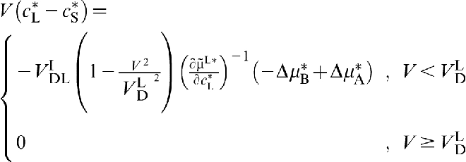
 ,
,  and
and  , i.e. complete solute trapping happens.

Molar Gibbs free energy diagram for isothermal solidification of binary alloys: if solute diffusion in solid is negligible at sharp interface, there are two independent dissipative processes, i.e. trans-interface diffusion and interface migration with fluxes respectively as
and  ;2,3 please see equations (26) and (27)
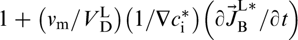
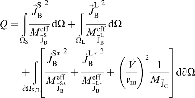
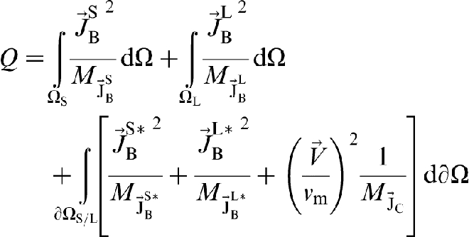
If the kinetic energy approach
13
is adopted, the total free energy dissipation Q is defined as
 and
and  , substituting equations (12) and (29) into equation (13) and then eliminating the Lagrange multiplier λ by equation (9) lead to the Maxwell–Cattaneo equation (equation (1)) for long range solute diffusion in bulk phases and
 (
( ) thereof is substituted by
  (
( ). Setting
  and using equation (9), equation (30) reduces to
If the interface dissipation by solute diffusion in solid (i.e. the first term in the brace of (equations (19) and (30)) reduce to the previous work, 3 which rederives the sharp interface model of Hillert et al.29,30 by TEP.31–37 The consideration of interface dissipation by solute diffusion in solid in the current work makes the sharp interface models equations (19) and (30) completely comparable with the phase field models21,23 as described in what follows.
Phase field modelling of rapid solidification of binary alloys
Phase field modelling of NESD upon rapid solidification of binary alloys was carried out recently.17,21,23 It was found that the kinetic energy approach 13 introduces the NESD to long range solute diffusion but not short range solute redistribution, thus resulting in an inhomogeneous solute profile within the interface even when diffusion less solidification has occured.17,21 The effective mobility approach 23 is able to introduce the NESD to both long range solute diffusion and short range solute redistribution and thus predicts an abruptly concurrent occurrence of complete solute trapping and absence of solute drag. To show clearly the difference between the kinetic energy approach 13 and the effective mobility approach 23 as well as the relation between phase field model and sharp interface model, the previous work21,23 is described concisely in what follows.
Total free energy and its change rate
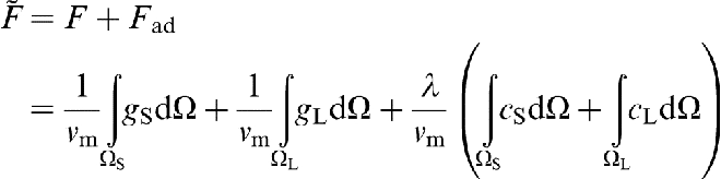
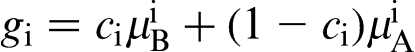
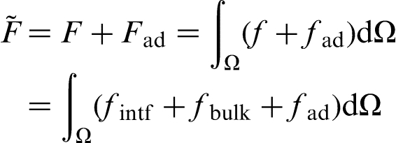
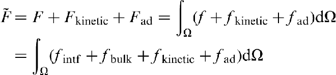
In the case of a diffuse interface, the generalised total free energy  in the entire volume Ω (see Fig. 4) is expressed as38,39

 ,
,  ) is the interpolation function,
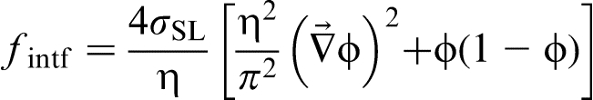
  is defined as the double obstacle potential
40
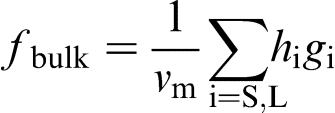
such that the interfacial width η remains finite uponsolidification, fbulk is assumed to be a mixture of gS and gL, and fad with the associated Lagrange multiplier λ is included such that the solute conservation is ensured to describe the additional constraint
is defined as the double obstacle potential
40
such that the interfacial width η remains finite uponsolidification, fbulk is assumed to be a mixture of gS and gL, and fad with the associated Lagrange multiplier λ is included such that the solute conservation is ensured to describe the additional constraint  thermodynamically consistently. The change rate of total free energy is
23
thermodynamically consistently. The change rate of total free energy is
23
 in equation (38)) is similar to that of interface migration at a sharp interface(e.g.
  in equation (8)). The conjugative driving force for solute diffusion
  can be rewritten as
  . The first term reduces to
  for solid where
  and
and  for liquid where
  (i.e. the driving forces for long-rage solute diffusion), whereas the second term corresponds to the driving forces for short range solute diffusion by noting that
  is similar to
  for short range solute diffusion at the sharp interface (see equation (8)). In other words, long and short range solute diffusions are integrated uniformly by phase field modelling but not described separately.
41
for short range solute diffusion at the sharp interface (see equation (8)). In other words, long and short range solute diffusions are integrated uniformly by phase field modelling but not described separately.
41

Schematic diagram for isothermal rapid solidification of binary alloys: in such diffuse interface separated by phase field
, the overall molar fraction c and solute diffusion flux  change continuously from boundary between interface and solid where
  and
and  to the boundary between interface and liquid where
  and
and 
The three dissipative processes are constrained by the solute balance that is given by the terms with the Lagrange multipliers λ in equation (37)
 with
with 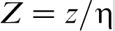 that is similar to
  in equation (10). The second term on the right hand side of equation (41) is the free energy production for long range solute diffusion in solid and liquid. The molar free driving energies from the bulk contribution are summarised in Fig. 5.
Molar Gibbs free energy diagram for isothermal solidification of binary alloys: if solute diffusion in solid is significant, there are three dependent dissipative processes (i.e. phase field propagation, solute diffusion in solid and liquid) and one additional constraint from solute balance within diffuse interface (i.e. equation (40)), which is similar to sharp interface as shown in Fig. 2
Adding the kinetic energy terms, i.e.  (
( ), to equation (33), we have
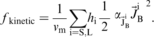
 (
( ),
13
the change rate of total free energy density is
21
),
13
the change rate of total free energy density is
21
 (
( ) from the kinetic energy is introduced to long range solute diffusion (i.e. the second term on the right hand side of equation (44)), whereas for phase field propagation, its free energy production is a non-bilinear expression in the flux and thermodynamic driving force (i.e. the first term on the right hand side of equation (44)). These outcomes are also comparable with the sharp interface equation (12).
Evolution equations
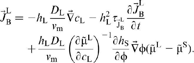
The evolution equations for the phase field propagation, solute diffusion in solid and liquid21,23 follow also the Onsager's reciprocal relation
31
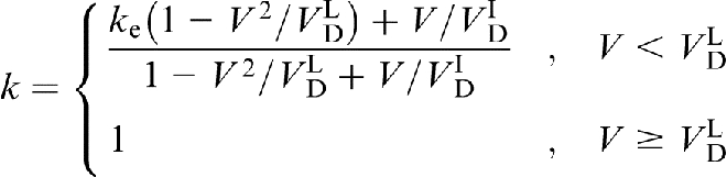
and are similar to equations (19) and (30) for sharp interface. In bulk phases, the governing equation for solute diffusion is the same as the Maxwell–Cattaneo evolution equation (equation (1)). In the case of negligible solute diffusion in solid, i.e. 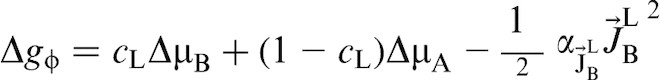 , the phase field model derived from the effective mobility approach
23
reduces to
, the phase field model derived from the effective mobility approach
23
reduces to
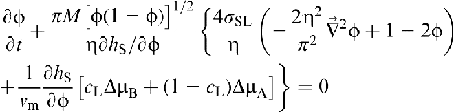
 and
and  . In the case of one-dimensional steady state growth, equation (46) in terms of the dimensionless coordinate
  reduces to
 . Furthermore, at
  ,
,  and
and  , i.e. complete solute trapping happens. Therefore, the effective mobility approach is able to predict a sharp concurrence of diffusionless solidification and absence of solute drag.
23
In this case, the local total molar driving free energy for phase field propagation and solute redistribution is
, i.e. complete solute trapping happens. Therefore, the effective mobility approach is able to predict a sharp concurrence of diffusionless solidification and absence of solute drag.
23
In this case, the local total molar driving free energy for phase field propagation and solute redistribution is  from the bulk contribution. The parts corresponding to the former and latter are respectively
  and
and  ; please see Fig. 6.
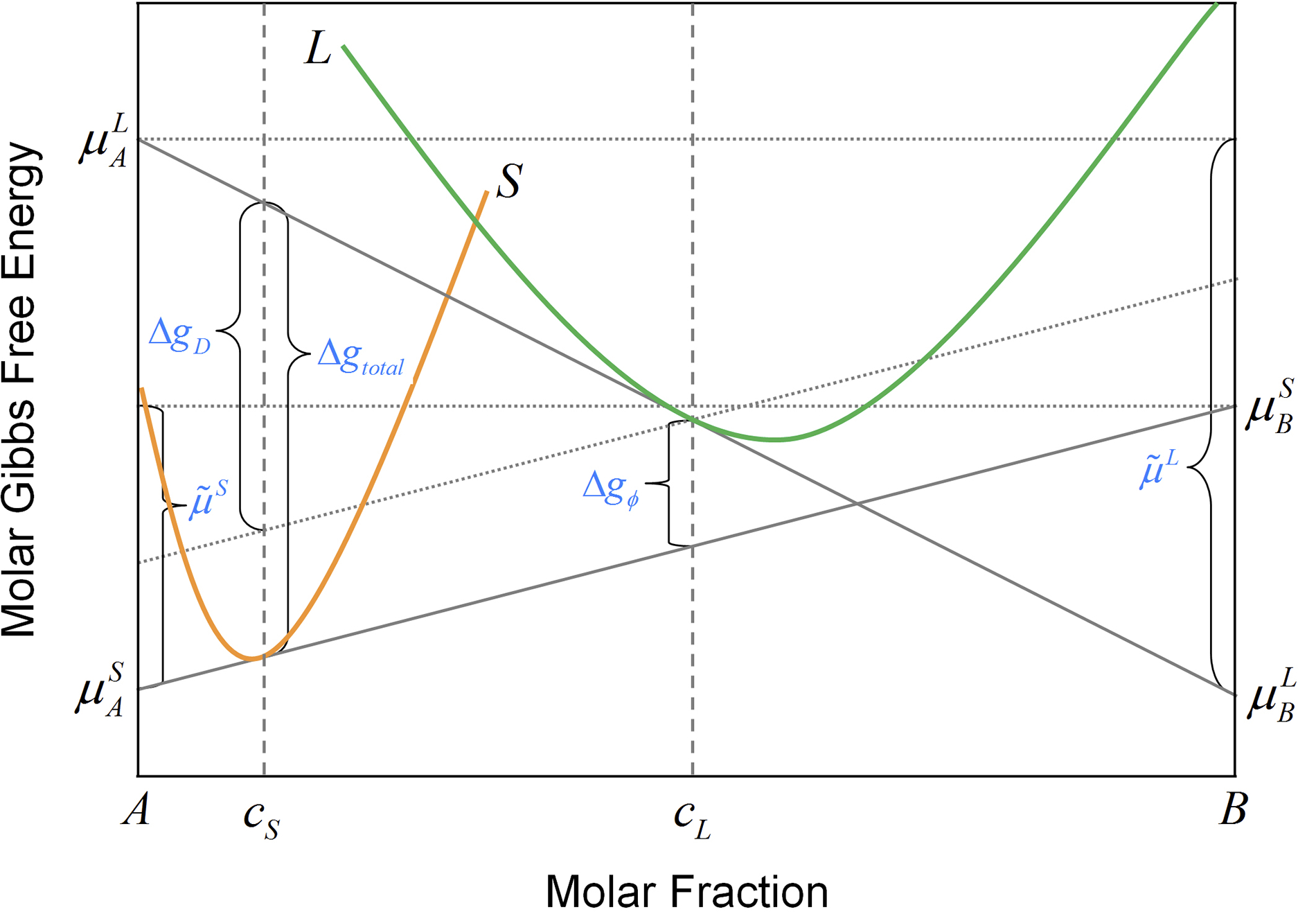
Molar Gibbs free energy diagram for isothermal solidification of binary alloys: if solute diffusion in solid is negligible, there are two independent dissipative processes, i.e. phase field propagation and solute diffusion in liquid; please see equations (45) and (46); two independent dissipative processes are totally comparable with interface migration and trans-interface diffusion at sharp interface as shown in Fig. 3
The phase field model derived from the kinetic energy approach
21
in the case of negligible solute diffusion in solid reduces to
 is similar to the case at the sharp interface (equation (31)).The NESD effect is introduced to long range solute diffusion (i.e. the second term on the right hand side of equation (49)) but not short range solute redistribution (i.e. the third term). This is the reason why solute diffusion still happens within the diffuse interface even at
  . For example, in the case of one-dimensional steady state growth, equation (49) in terms of the dimensionless coordinate
  reduces to
 . However,
  holds at
  , i.e. complete solute trapping
  occurs.
Conclusions
The effective mobility approach
23
is compared with the kinetic energy approach
13
in terms of sharp interface modelling and phase field modelling of NESD upon rapid solidification of binary alloys. The current work is helpful not only for modelling of NESD but also for understanding of non-equilibrium phenomena (e.g. in undercooled metals).
42
Our main conclusions are as follows.
The effective mobility approach
23
introduces the NESD effect to both long range solute diffusion in bulk phases and short range solute diffusion at the sharp interface or within the diffuse interface. It allows complete solute trapping in the case when a sharp interface happens abruptly at a finite interface velocity that is equal to the solute diffusion velocity in liquid, and in the case when a diffuse interface occurs together with the absence of solute drag. The kinetic energy approach
13
includes the NESD effect into long range solute diffusion but not short range solute diffusion either at the sharp interface or within the diffuse interface. For the sharp interface modelling, it needs to be combined with the effective diffusion coefficient of Sobolev,
10
which is a special case of effective mobility to predict complete solute trapping. For phase field modelling, it allows complete solute trapping to happen at a finite interface velocity but with unreasonable solute diffusion within the interface. As a useful principle for modelling of non-equilibrium dissipative systems with additional constraints, the TEP of Svoboda et al.34–37 is adopted to derive the evolution equations. Compared with the kinetic energy approach,
13
which results in a non-bilinear expression in the flux and thermodynamic driving force in the free energy production of interface migration (equation (12)) or of phase field propagation (equation (44)), the effective mobility approach
23
allows the TEP of Svoboda et al.34–37 workable for modelling of NESD without any arbitrary approximation.
Acknowledgements
Haifeng Wang thanks the support of Alexander von Humboldt Foundation for a research fellowship and Professor P. K. Galenko for useful discussions. Authors are grateful to the National Basic Research Program of China (973 Program, grant no. 2011CB610403), National Science Funds for Distinguished Young Scientists (grant no. 51125002), Natural Science Foundation of China (grant no. 51371149), the Fundamental Research Funds for the Central Universities (No. 3102015AX003) and Free Research Fund of State Key Lab. of Solidification Processing (grant no. 92-QZ-2014).