
Abstract
Phase transformation with a moving interface occurs under far from local equilibrium conditions when the interface moves with sufficiently high velocity. This deviation cannot be adequately described by the classical irreversible thermodynamics with diffusion equation of parabolic type because it assumes local equilibrium hypothesis. The local non-equilibrium diffusion model has been developed to take into account the deviation from local equilibrium during binary alloy solidification using the hyperbolic diffusion equation. The model introduces a finite propagation velocity of concentration disturbances in the bulk liquid VD as the characteristic diffusion parameter and predicts a sharp transition from diffusion controlled to diffusionless and partitionless solidification at V = VD due to the deviation from local equilibrium. This review does not intend to be extensive, but rather to illustrate the main advances of the local non-equilibrium diffusion approach in rapid alloy solidification. Applications of the local non-equilibrium model to other phase transformation processes such as solid–solid transformation, colloidal and multicomponent alloy solidification have been briefly discussed. The parallels and possible combinations of the model with molecular dynamics, phase field, phase field crystal and cellular automata methods have been considered.
Keywords
Introduction
The modelling of phase transformation with moving phase interface such as binary and multicomponent alloy solidification, colloidal solidification and solid state transformation typically considers the transport of mass and heat through the bulk of the one or both of the phases as well as the phase transformation kinetics at the interface.1–6 In the near equilibrium limit, transformation occurs slowly enough that the growing phase has the equilibrium composition, given by the equilibrium phase diagram. But when the interface velocity V increases, the transformation process begins to deviate from equilibrium.1–97 The non-equilibrium nature of phase transformation has made it possible to produce supersaturated solid solutions, metastable compounds, highly disordered intermetallic compounds, ceramic materials, glasses and other advanced engineering materials with unique characteristics.1–97 The most obvious manifestation of the deviation from local equilibrium during rapid alloy solidification is solute trapping, which reduces the solute segregation at the solid/liquid interface.1–37 The solute trapping phenomenon is often accompanied by grain refinement7–9,11,14–17 and is analogous to disorder trapping14–17 and density trapping.
38
Therefore, the development of capability in predicting solute trapping phenomena, especially at far from local equilibrium conditions, is an important task in designing new materials and new processes. The degree of solute trapping is usually quantified by the partition coefficient K, defined as the ratio of the concentration of solute in the solid CS to that in the liquid CL at the interface. Several models of the solute trapping during solidification of binary alloys have been proposed.18–37 Continuous growth model (CGM) by Brice
33
and Aziz et al.34,35 (see also discussion in Ref. 36) leads to the following K versus V dependence
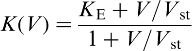
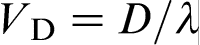 , where D is the solute diffusion coefficient in the bulk liquid, and λ is the interatomic spacing. In this case, the characteristic solute trapping velocity is given as
 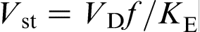 , where f is a fraction of solute atoms that reach the solid surface and join the solid phase, i.e. a fraction of active surface growth sites. The model of Aziz et al. treats Vst as the interface diffusive velocity Vi, which was given by the ratio Di/λ, where Di is the coefficient for interdiffusion across the interface, and λ is the interatomic spacing
34
or the interface width.
35
In spite of some arbitrariness about how Vi is treated, it can be considered as a solute partitioning parameter, which is the growth rate at which K(V) is in midtransition between KE and unity.
35
Both Di and Vi are not subject to direct experimental determination: the values for Vi have been inferred by fitting the observed dependence of K on V.
35
Assuming that Vst is identical for both models, we obtain
, where f is a fraction of solute atoms that reach the solid surface and join the solid phase, i.e. a fraction of active surface growth sites. The model of Aziz et al. treats Vst as the interface diffusive velocity Vi, which was given by the ratio Di/λ, where Di is the coefficient for interdiffusion across the interface, and λ is the interatomic spacing
34
or the interface width.
35
In spite of some arbitrariness about how Vi is treated, it can be considered as a solute partitioning parameter, which is the growth rate at which K(V) is in midtransition between KE and unity.
35
Both Di and Vi are not subject to direct experimental determination: the values for Vi have been inferred by fitting the observed dependence of K on V.
35
Assuming that Vst is identical for both models, we obtain 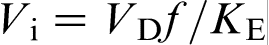 , which corresponds to experimentally observed inverse correlation between Vi and KE.
35
, which corresponds to experimentally observed inverse correlation between Vi and KE.
35
According to the most recent solute trapping theory of Jackson et al.,
37
K(V) is described as a power law given as
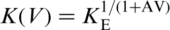
Local non-equilibrium diffusion approach to rapid alloy solidification
Local non-equilibrium diffusion model (LNDM): Simplest version
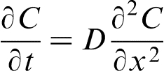
There exists an extensive body of literature on the heat mass transfer theories that go beyond the local equilibrium assumption (see, for example, Refs. 39–44 and references therein). The extended irreversible thermodynamics
39
is one of the most elaborated versions of the thermodynamic theories. It is remarkable that all these approaches lead to the hyperbolic diffusion equation (HDE) as the first step generalisation of PDE for the local non-equilibrium case
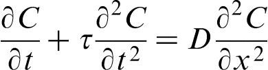
 .18–32,39–44 When
  , HDE reduces to PDE, which implies an infinite velocity of concentration disturbances
 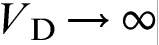 . The local equilibrium assumption holds for relatively slow processes when the characteristic time of the process tchand breaks down for fast processes when
 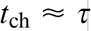 . In terms of the solid/liquid interface velocity V, the local equilibrium assumption holds at
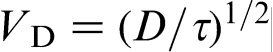
 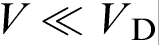 and breaks down at V∼VD. In the last case, the diffusion process occurs under far from local equilibrium conditions, and it should be described by HDE (equation (3)).18–22,39–44 For metallic alloys, VD is of the order 10–20 m s− 1,7–9,11 whereas for intermetallic compounds, it is in the range from 0.2 to 3.8 m s− 1.12,14–17 Note that the diffusion velocity VD defined by HDE as the speed of concentration wave (concentration disturbances) in the bulk liquid is a purely diffusion parameter. In contrast, the interface diffusive velocity Vi in CGM characterises the solute segregation at the interface and is a solute trapping parameter. To stress the difference between Vi and VD, we sometimes call the later as the bulk liquid diffusion velocity.18–22
In the context of the moving phase transformation zone, HDE has been first used to describe temperature distribution around the ultrafast moving energy source (see Ref. 40 and references wherein). Later, this approach has been modified to develop the LNDM18–22 for rapid solidification of binary alloys, which takes into account the local non-equilibrium solute diffusion in the bulk liquid at high interface velocity V∼VD.
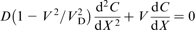
The exact mathematical treatment of the solute diffusion problem may be found by solving the time dependent HDE (equation (3)), subject to appropriate initial and boundary conditions in both the solid and the liquid phases. But to avoid mathematical difficulties, the steady state approximation is usually used. It assumes that, after a short initial transient period, the solid/liquid interface begins to move with constant velocity V, and the solute concentration is time independent in the reference frame attached to the interface. In the steady state approximation, equation (3) gives18–27,40
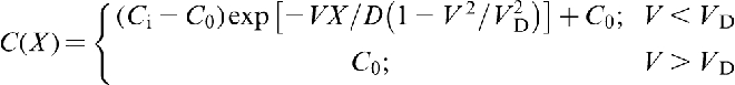
 and at the interface (X = 0) respectively. Equation (5) predicts that the local non-equilibrium diffusion effects qualitatively change the solute diffusion head of the fast moving interface: the solute diffusion field remains undisturbed at V ≥ VD. This result has a clear physical meaning: a source of concentration disturbances, i.e. the interface, moving with a velocity higher than the maximum velocity of the disturbances, i.e. the diffusive velocity VD, cannot affect the media ahead of itself.
40
This phenomenon is analogous to supersonic effect. Thus, when the interface velocity V exceeds the critical point V = VD, the local non-equilibrium diffusion effects lead to an abrupt transition from diffusion controlled to diffusionless solidification.18–22 Figure 1 plots the steady state local non-equilibrium concentration profiles around the interface region (equation (5)), for different ratios V/VD (solid curves). The corresponding local equilibrium solute concentration distributions
and at the interface (X = 0) respectively. Equation (5) predicts that the local non-equilibrium diffusion effects qualitatively change the solute diffusion head of the fast moving interface: the solute diffusion field remains undisturbed at V ≥ VD. This result has a clear physical meaning: a source of concentration disturbances, i.e. the interface, moving with a velocity higher than the maximum velocity of the disturbances, i.e. the diffusive velocity VD, cannot affect the media ahead of itself.
40
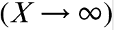
This phenomenon is analogous to supersonic effect. Thus, when the interface velocity V exceeds the critical point V = VD, the local non-equilibrium diffusion effects lead to an abrupt transition from diffusion controlled to diffusionless solidification.18–22 Figure 1 plots the steady state local non-equilibrium concentration profiles around the interface region (equation (5)), for different ratios V/VD (solid curves). The corresponding local equilibrium solute concentration distributions  obtained from PDE (see, for example, Refs. 1 and 2) are placed for comparison. When V < VD (Fig. 1a and b), there is a concentration spike C(X)>C0 ahead of the interface due to the solute segregation at the interface and solute diffusion in the bulk liquid. In such a case, the solidification mechanism is essentially controlled by solute diffusion. As the interface velocity increases, the local non-equilibrium diffusion effects became more significant, and the concentration spike is getting smaller and narrower (compare solid and dashed lines in Fig. 1a and b). When the interface velocity V exceeds the diffusion velocity VD, the solute diffusion ahead of the moving interface is totally depressed by the local non-equilibrium effects and the solute concentration in the liquid phase does not change, i.e. and C(X) ≡ C0 (see solid line in Fig. 1c). In contrast, the local equilibrium models1,2 predict that the diffusion layer and the concentration spike at the interface exist even at V>VD (see dashed line in Fig. 1c). The value of the local non-equilibrium characteristic diffusing length (boundary layer) δLNDM is defined by equation (5) as18–22 (see curve 3 in Fig. 2)
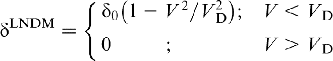
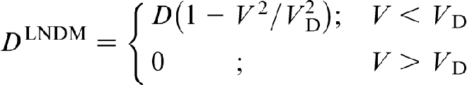
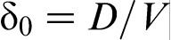 is the characteristic diffusion length for the local non-equilibrium case1,2 (curve 4 in Fig. 2). As interface velocity V increases, the effective diffusion length δLNDM (equation (6)), shrinks more rapidly than δ0 and equals zero at V>VD, whereas δ0>0 at any value of V (see curves 3 and 4 in Fig. 2). A comparison of the local non-equilibrium solute distribution ahead of the moving interface (equation (5)) with the local equilibrium one allows us to introduces the effective (velocity dependent) diffusion coefficient in the form18–22
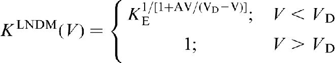
 , when the interface velocity V passes through the critical point V = VD (curve 5 in Fig. 2).18–29 The result is in agreement with experimental data19,20,22 and has been confirmed by molecular dynamics (MD),58–60 phase field (PF) model
61
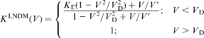
and phase field crystal (PFC) model.62–64 Note that the local equilibrium models (equations (1) and (2)) predict complete solute trapping K → 1 only asymptotically at V → ∞ (curve 1 in Fig. 2). Substituting D for DLNDM in the non-dilute CGM expression for partition coefficient,
36
one can easily obtain the non-dilute LNDM partition coefficient in the form24,25
, when the interface velocity V passes through the critical point V = VD (curve 5 in Fig. 2).18–29 The result is in agreement with experimental data19,20,22 and has been confirmed by molecular dynamics (MD),58–60 phase field (PF) model
61
and phase field crystal (PFC) model.62–64 Note that the local equilibrium models (equations (1) and (2)) predict complete solute trapping K → 1 only asymptotically at V → ∞ (curve 1 in Fig. 2). Substituting D for DLNDM in the non-dilute CGM expression for partition coefficient,
36
one can easily obtain the non-dilute LNDM partition coefficient in the form24,25
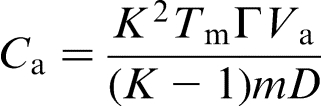
 at a given Ca, which implies that the local non-equilibrium diffusion effects stabilise the interface due to depressed solute diffusion. Moreover, the local non-equilibrium diffusion effects set the limit
 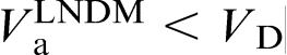 .19,20,22
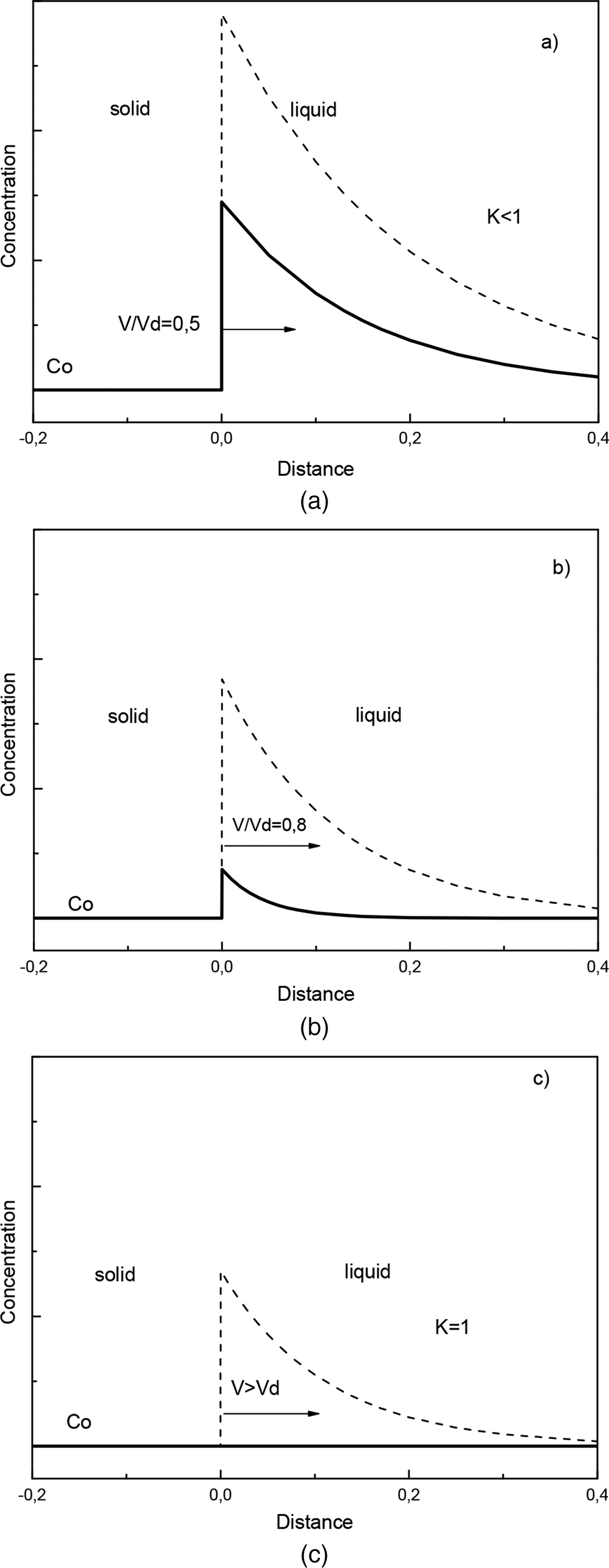
a V/VD = 0·5: long range diffusion growth; b V/VD = 0·9: short range diffusion growth; c V>VD: diffusionless growthConcentration profiles near interface region versus position obtained at different values of non-dimensional interface velocity V/VD [solid lines: prediction of LNDM with HDE (eq. (5); dashed lines: prediction of PDE (VD → ∞)]

Local equilibrium partition coefficient K, equations (1) and (2) (curve 1); non-dimensional effective diffusion coefficient DLNDM/D, equation (7) (curve 2); non-dimensional local non-equilibrium boundary layer δLNDM, equation (6) (curve 3); non-dimensional local equilibrium boundary layer
(curve 4); and local non-equilibrium partition coefficient KLNDM, equation (8) (curve 5) as functions of non-dimensional interface velocity V/VD
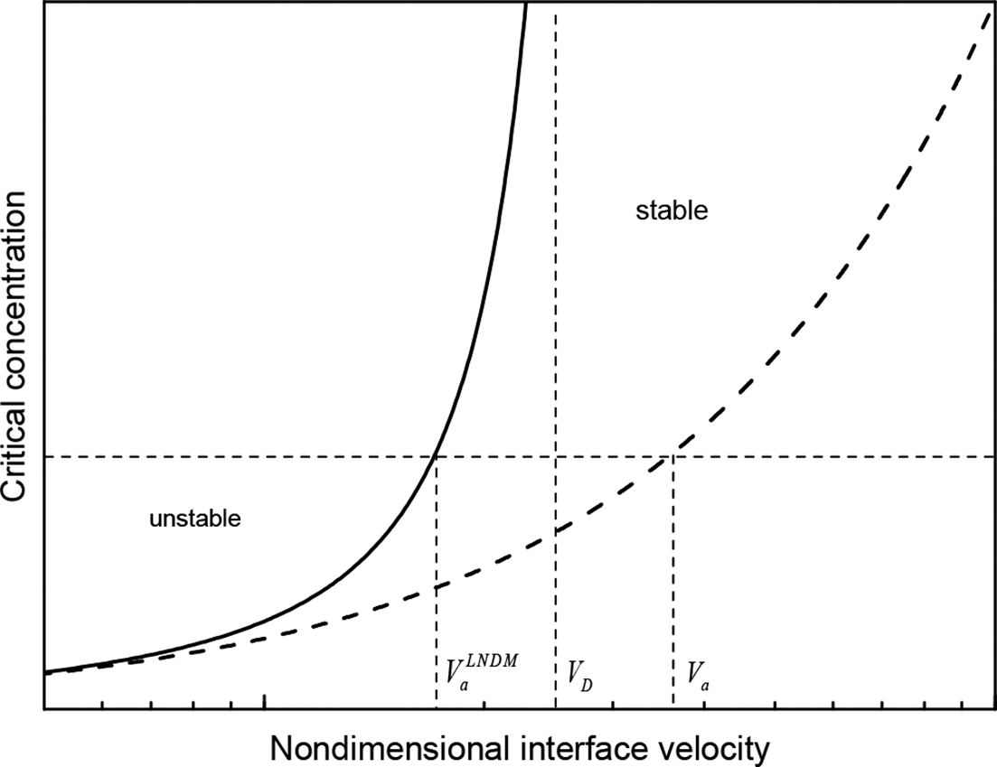
Critical concentration Ca as function of non-dimensional velocity Va/VD (solid curve: prediction of LNDM; dashed curve: local equilibrium Mullins and Sekerka theory)
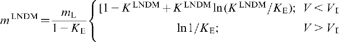
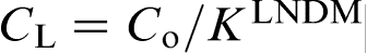
The slope of the local non-equilibrium liquidus line mLNDM can be written as19–22
 and
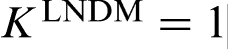
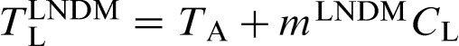
and  respectively, where TA is the melting temperature of the major component. As the interface velocity V increases, the effective solidus temperature increases, and the effective liquidus temperature decreases due to the solute trapping effects. At V = VD (when KLNDM = 1), they coincide reaching the T0 temperature, i.e. the temperature of equal free energy of two phases, and at V>VD, they do not change any more. The interface temperature for steady state planar growth with allowance for local non-equilibrium effects is given as

 (curve 1) and for the fixed solute concentration at the interface in the liquid
 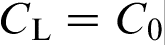 (curve 2). The sharp change in the effective partition coefficient KLNDM (equation (8) or (9)), during the transition to diffusionless solidification at
  leads to the corresponding sharp change in the effective liquidus slope mLNDM (equation (10)), which, in turn, leads to the sharp break of the interface temperature versus interface velocity function
  (equation (11)). At
  , the growth is mainly solute diffusion controlled (second term on the right hand side of equation (11)). When the interface velocity V exceeds the critical point
  , equation (11) can be rewritten in terms of T0 temperature as
  , which implies that, at these velocities, the alloy solidifies as a ‘pure metal’ with melting temperature T0. The transition to diffusionless and partitioned solidification occurs at
  , i.e. rather close to the T0 line.19–22,27 The prediction of LNDM that the local non-equilibrium diffusion effects lead to the sharp transition from diffusion controlled solidification to diffusionless and partitionless growth at
  , which is accompanied by the break in the
  function, is consistent with experimental data.7–17,19–27 For example, measurements of interface velocity as a function of undercooling during rapid solidification of Cu–Ni and Cu–Ni–B,7,8 Ni–B,9,11,14 Ag–Cu,
10
Co–Si,11,12,14 Ti–Ni,
13
Fe–Ge (Ref. 16) and β Ni3Ge (Ref. 17) reveal a sharp break in the velocity–undercooling relationship at relatively high interface velocity, which is accompanied by almost partitionless solidification.9,11 The experiments show that it is not the critical undercooling that initiates the break, but rather the critical solidification velocity, which approximately equals the diffusive speed VD. Note that the classical solidification approach based on PDE can describe the transition to diffusionless solidification with complete solute trapping only asymptotically at V → ∞.
function, is consistent with experimental data.7–17,19–27 For example, measurements of interface velocity as a function of undercooling during rapid solidification of Cu–Ni and Cu–Ni–B,7,8 Ni–B,9,11,14 Ag–Cu,
10
Co–Si,11,12,14 Ti–Ni,
13
Fe–Ge (Ref. 16) and β Ni3Ge (Ref. 17) reveal a sharp break in the velocity–undercooling relationship at relatively high interface velocity, which is accompanied by almost partitionless solidification.9,11 The experiments show that it is not the critical undercooling that initiates the break, but rather the critical solidification velocity, which approximately equals the diffusive speed VD. Note that the classical solidification approach based on PDE can describe the transition to diffusionless solidification with complete solute trapping only asymptotically at V → ∞.

Non-dimensional interface temperature T/TA versus non-dimensional interface velocity V/VD: curve 1, steady state, i.e.
at interface; curve 2,  at interface
The transition from diffusion controlled to thermally controlled growth with the sharp break in the  (or interface velocity versus interface undercooling) function is often accompanied by disorder trapping and grain refinement.7–9,11,14–17 Disorder trapping is a phenomenon quite analogous to solute trapping: at high interface velocity, the atoms can no longer sort themselves by diffusion to build up the superlattice of the intermetallic phase, which leads to a disordered structure. This implies that the local non-equilibrium diffusion effects set the limit Vcrit < VD on the critical velocity Vcrit at which an ordered structure can still form. Indeed, at V>VD, there is no diffusion ahead of the interface, and an ordered structure cannot form at such velocity. Moreover, estimates of a solute boundary layer under local non-equilibrium conditions demonstrate that, if one or two diffusive jumps of solute atoms are needed to build up the superlattice, the critical velocities are Vcrit = 0.6VD or Vcrit = 0.4VD respectively.
27
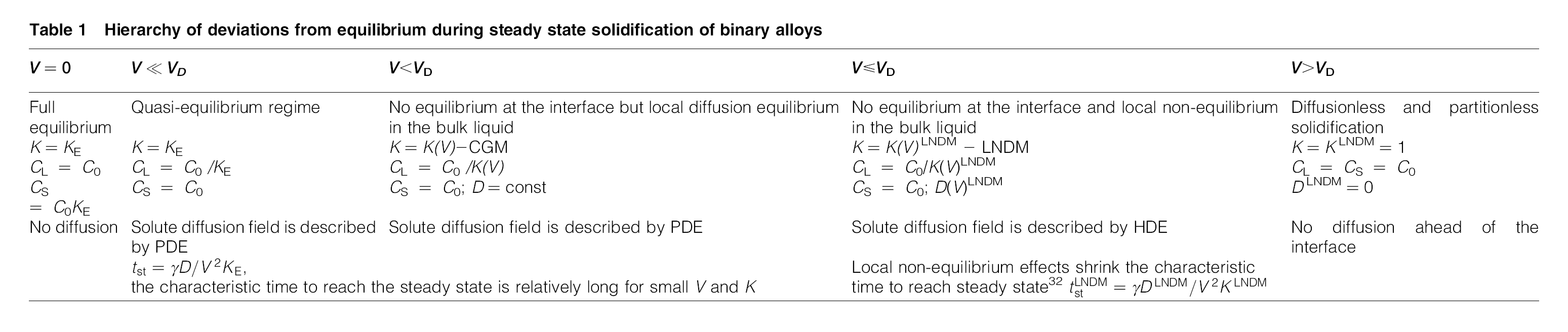
Thus, as the interface velocity increases, the deviation from equilibrium also increases, which affects the solute partitioning at the interface and solute diffusion in the bulk liquid. The hierarchy of deviations from equilibrium with increasing interface velocity V is summarised in Table 1.
(or interface velocity versus interface undercooling) function is often accompanied by disorder trapping and grain refinement.7–9,11,14–17 Disorder trapping is a phenomenon quite analogous to solute trapping: at high interface velocity, the atoms can no longer sort themselves by diffusion to build up the superlattice of the intermetallic phase, which leads to a disordered structure. This implies that the local non-equilibrium diffusion effects set the limit Vcrit < VD on the critical velocity Vcrit at which an ordered structure can still form. Indeed, at V>VD, there is no diffusion ahead of the interface, and an ordered structure cannot form at such velocity. Moreover, estimates of a solute boundary layer under local non-equilibrium conditions demonstrate that, if one or two diffusive jumps of solute atoms are needed to build up the superlattice, the critical velocities are Vcrit = 0.6VD or Vcrit = 0.4VD respectively.
27
Thus, as the interface velocity increases, the deviation from equilibrium also increases, which affects the solute partitioning at the interface and solute diffusion in the bulk liquid. The hierarchy of deviations from equilibrium with increasing interface velocity V is summarised in Table 1.
Hierarchy of deviations from equilibrium during steady state solidification of binary alloys
Extensions of LNDM
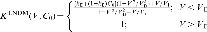
Local non-equilibrium diffusion model,18–22 briefly referred to in the previous section, is the simplest model to describe the local non-equilibrium diffusion effects during rapid solidification of binary alloys. It assumes that the plane interface is sharp and the liquidus and solidus are linear lines. Many recent papers3–5,23–32,45–56 extend LNDM to more general cases. A number of solute trapping models beside CGM have been modified for the local non-equilibrium case using the effective diffusion coefficient (equation (7)).24,25 All the modified models predict complete solute trapping K = 1 at V>VD due to depressed solute diffusion 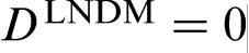 (see equation (7)). The dimensionless growth parameter found in the Monte Carlo simulations as the important parameter for solute trapping
37
has been modified for the local non-equilibrium diffusion case taking into account that the probability that an atom will be trapped into the crystal under local non-equilibrium conditions depends on V
D
.
26
In such a case, the Jackson et al. model (equation (2))
37
yields
26
(see equation (7)). The dimensionless growth parameter found in the Monte Carlo simulations as the important parameter for solute trapping
37
has been modified for the local non-equilibrium diffusion case taking into account that the probability that an atom will be trapped into the crystal under local non-equilibrium conditions depends on V
D
.
26
In such a case, the Jackson et al. model (equation (2))
37
yields
26
Applications to other systems
Multicomponent alloy solidification
All the above analysis focuses on binary alloys, while most industrial alloys are multicomponent alloys.29,66–71,94,96 Local non-equilibrium diffusion model version for multicomponent alloys
29
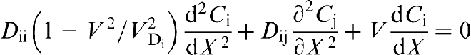
leads to the solute diffusion equations in the form
 diffusion matrix. In general, the diffusion coefficients are not symmetric
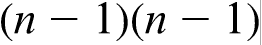
 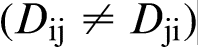 . The diagonal terms Dii are so called the ‘main terms’ of the diffusion matrix because they are commonly larger than the off-diagonal terms Dij and similar in magnitude to the binary values.
For a steady state growth of a ternary system  with plane interface, equation (13) reduces to
29
with plane interface, equation (13) reduces to
29
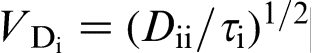 . If the diffusional interaction between the species is ignored, the solute distributions are independent from each other, and a two-step transition to diffusionless solidification occurs: at
 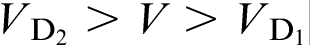 , the growth is partly diffusionless, i.e. it is diffusionless with regards to the solute 1, and at
 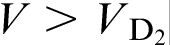 , the growth is completely diffusionless. At a relatively weak diffusional interaction, the solute concentrations ahead of the interface change monotonically with the distance, but a strong interaction between the components may lead to a maximum or a minimum of solute concentrations in the liquid phase.29,68 Diffusion velocity values in the multicomponent systems change due to the interaction between the components,
29
which, in turn, changes condition for solute trapping at the interface. Wang et al.70,71 modified the local non-equilibrium approach to the multicomponent concentrated alloys. For the time being, however, use of analytical solutions is limited by the lack of measured diffusion coefficients and methods to determine the off-diagonal terms.
, the growth is completely diffusionless. At a relatively weak diffusional interaction, the solute concentrations ahead of the interface change monotonically with the distance, but a strong interaction between the components may lead to a maximum or a minimum of solute concentrations in the liquid phase.29,68 Diffusion velocity values in the multicomponent systems change due to the interaction between the components,
29
which, in turn, changes condition for solute trapping at the interface. Wang et al.70,71 modified the local non-equilibrium approach to the multicomponent concentrated alloys. For the time being, however, use of analytical solutions is limited by the lack of measured diffusion coefficients and methods to determine the off-diagonal terms.
Solid state transformations
Solid state transformation is receiving increasing interest in the material science community both from experimental and theoretical point of view.3,36,72,73,93 Solid state transformations provide an interesting setting to test theoretical models in new regimes that are not usually accessible in a solidification context, such as the transitions to absolute morphological stability and to diffusionless solidification with complete solute trapping at high interface velocity. As the critical velocities required for transition to absolute stability Va and to diffusionless (and partitionless) solidification VD are proportional to the solute diffusion coefficient, these typical velocities are very high in alloy solidification and very difficult to produce. The solid state diffusion coefficients, and hence the critical velocities in solid state transformations, are orders of magnitude smaller and can be easily reached. For example, in directional transformation of a hypoperitectic Fe–17.5 at-Co alloy, flat cells were observed at 7 μm s− 1, while the plane front γ was clearly seen at 10 μm s− 1.
72
The authors concluded that the experimentally determined Va value is between these two growth rates, which agrees well with the calculated value of Va = 9.2 μm s− 1 obtained from the local equilibrium theory with  . At relatively low interface velocity V = 1 μm s− 1, the concentration spike was observed at δ/γ interface, but at higher rate V = 10 μm s− 1, no concentration spike was detected.
72
However, it was concluded that a spike existed according to classical approach, but it was not detected with the electron probe micro-analyser (EPMA) technique because it was very thin. It should be stressed that there is an appreciable uncertainty in the experimental values of the diffusion coefficient in Fe–Co system. For example, assuming
. At relatively low interface velocity V = 1 μm s− 1, the concentration spike was observed at δ/γ interface, but at higher rate V = 10 μm s− 1, no concentration spike was detected.
72
However, it was concluded that a spike existed according to classical approach, but it was not detected with the electron probe micro-analyser (EPMA) technique because it was very thin. It should be stressed that there is an appreciable uncertainty in the experimental values of the diffusion coefficient in Fe–Co system. For example, assuming  , we obtain VD = 8 μm s− 1, which is less than the higher rate V = 10 μm s− 1 obtained in the experiment.
72
This implies that at V = 10 μm s− 1, the diffusionless transformation regime with complete solute trapping was reached in the experiment. The absence of a concentration spike at δ/γ interface (Fig. 6b in Ref. 72) corresponds to this conclusion. The authors
72
also proposed that the interface velocity must be >10 cm s− 1 to reach the regime of complete solute trapping, whereas LNDM predicts VD = 0.825 cm s− 1 at the same value of the diffusion coefficient, which is at least one order of magnitude lower. Using the Gibbs energy dissipation approach, Hillert et al.36,73 estimated that the partitionless growth of α (bcc) phase from γ (fcc) phase in the FeNi system at 900 K and an alloy composition of 6 mol.-Ni can be reached at a velocity ∼10− 12 m s− 1. This approach also predicts that diffusionless and partitionless transformation can occur rather close to the T0 line, which corresponds to our prediction
, we obtain VD = 8 μm s− 1, which is less than the higher rate V = 10 μm s− 1 obtained in the experiment.
72
This implies that at V = 10 μm s− 1, the diffusionless transformation regime with complete solute trapping was reached in the experiment. The absence of a concentration spike at δ/γ interface (Fig. 6b in Ref. 72) corresponds to this conclusion. The authors
72
also proposed that the interface velocity must be >10 cm s− 1 to reach the regime of complete solute trapping, whereas LNDM predicts VD = 0.825 cm s− 1 at the same value of the diffusion coefficient, which is at least one order of magnitude lower. Using the Gibbs energy dissipation approach, Hillert et al.36,73 estimated that the partitionless growth of α (bcc) phase from γ (fcc) phase in the FeNi system at 900 K and an alloy composition of 6 mol.-Ni can be reached at a velocity ∼10− 12 m s− 1. This approach also predicts that diffusionless and partitionless transformation can occur rather close to the T0 line, which corresponds to our prediction  .19–22,27 Thus, owing to the small diffusion coefficients in solids, and hence low corresponding diffusion velocity, the solid state transformation appears to be a promising field to experimental study of local non-equilibrium diffusion effects.
Colloidal solidification
In materials science, the rapid solidification of colloidal or nanosuspensions is receiving increasing interest owing to the novel microaligned structures that can be produced for a wide range of applications such as organic electronics, microfluidics, molecular filtration, nanowires, cryopreservation and tissue engineering.23,74–78 Using the freezing of colloids to template the porosity in materials is known as ice templating or freeze casting.
74
The phenomenon is very similar to unidirectional solidification of binary alloys, with ice playing role of a fugitive second phase. Typical velocities used when processing materials through solidification of colloidal suspensions are of the order of 10–100 μm s− 1, which implies that the system in these conditions is likely to be out of equilibrium.23,74–78 The investigation of the structure and dynamics of the crystal/fluid interface of colloidal hard spheres in real space by confocal microscopy demonstrates that the deviation from equilibrium leads also to the interface broadening from 8 to 9 particle diameters close to equilibrium to 15 particle diameters far from equilibrium.
78
The diffusive speed VD in colloidal solidification can be treated as the maximum speed with which an individual particle moves in the bulk liquid, i.e. the ‘molecular’ velocity of the particles, which depends on the particle size.23,75 For alumina particle size of 2–20 μm, the estimated diffusion velocity falls in the range of 10–125 μm s− 1,
23
which can be likely of the order of the experimentally observed interface velocity in colloidal solidification.
76
Partitioning of polystyrene impurity particles during colloidal solidification has been studied by Nozava et al.
77
It was observed that, for each sample with different impurities, K approached unity as the growth rate increased. The diffusion coefficient of each particle was determined using the Stokes–Einstein equation, and the results were found to be similar for the different particles and on the order of 10− 12 m2 s− 1. Assuming that the particle jump distance in the liquid phase is of the order of the host particles size R = 500 nm, the diffusion velocity can be estimated as  , which gives VD = 7.2 mm h− 1. This value corresponds to the critical velocity for complete solute trapping observed in the experiment.
77
Thus, the low values of diffusion velocity and the big size of colloidal particles make colloidal suspensions increasingly important as model systems to study local non-equilibrium phase transformations.
, which gives VD = 7.2 mm h− 1. This value corresponds to the critical velocity for complete solute trapping observed in the experiment.
77
Thus, the low values of diffusion velocity and the big size of colloidal particles make colloidal suspensions increasingly important as model systems to study local non-equilibrium phase transformations.
Parallels and combination with other approaches
Molecular dynamics simulations
In recent years, a fundamental understanding of alloy solidification has been gained through MD.1,2,58–60,79,80 Cook and Clancy58,59 have used non-equilibrium MD simulation method to study solute trapping in an AxB1 − x Lennard–Jones alloy. The complete solute trapping was found when the interface velocity attained its steady state value of 4 m s− 1. It has been stressed that neither the CGM nor periodic stepwise growth theories of solute segregation, which are based on CIT, predicted the complete trapping observed in the MD simulations. The most recent work Yang et al. 60 calculated solute concentration profile around the interface region from an “LJ simulation with a relatively low velocity and the highest velocity considered. For the slow V, the concentration profile demonstrates a peak on the liquid side of the interface, which corresponds to LNDM predictions at V < VD. For the high V case, the MD simulation results in the nearly flat concentration profile, indicating clearly solute trapping behaviour (Fig. 1 in Ref. 60), which is consistent with diffusionless solidification predicted by LNDM at V>VD. Yang et al. 60 also calculated solute partition coefficient K versus V and compared the result with theoretical models. Continuous growth model and the model of Jackson et al. fit the data only for the lower velocities. At higher interface velocity, the MD date of Yang et al. 60 predicts transition to partitionless solidification at a finite value of the interface velocity (see the upper panel of Fig. 2 in Ref. 60), which is in agreement with LNDM predictions18–27 (see also equations (8) and (12)) and cannot be explained in the frameworks of CGM and the model of Jackson et al.
In recent years, particular interest has centred on the hybrid continuum atomistic models of laser–materials interactions, which combine the advantages of MD method with a continuum description.79,80 Molecular dynamics is used in the very phase transformation region, where active processes of rapid non-equilibrium phase transformations, damage and ablation take place, whereas the continuum equations are solved in a much wider region affected by the heat mass transfer in the system. In particular, the local non-equilibrium phase transformations in metals have been studied by MD simulations combined with the continuum two-temperature (2T) model.79,80 The continuum 2T model has been widely used to describe energy transfer in metals under ultrashort laser irradiation.41,44,79,80,90 It assumes that the lattice and electrons can be described by separate temperatures, which space–time evolution is described by two coupled heat conduction equations. The parabolic 2T model, which assumes that the electron gas is at local equilibrium, uses the classical transfer equation of parabolic type for the electron gas. For far from local equilibrium processes, when the relaxation time of the electrons is of the order of the characteristic time of the process (e.g. the laser pulse duration), the hyperbolic 2T model41,44,90 should be used. A combination of the hyperbolic 2T model with MD methods provides better description of ultrafast laser beam interaction with metals. 79
Phase field models
The PF models consider the diffuse character of the solid/liquid interface with a finite thickness and describe the dynamical phenomena in both the bulk phases and the interface region by the minimisation of some specified free energy functional.1,2,61,81–85 The jump in the concentration at the interface, which is typical for a sharp interface formulation disappears and is replaced by a continuous profile. The detailed description of the interface region seems to be more realistic, but it is achieved at the expense of rather complicated mathematical formulation. Phase field studies with the parabolic form of the dynamic equations1,2,81–84 have been modified to their hyperbolic form using HDE (equation (3)), for solute concentration and PF variables.61,85 The hyperbolic PF model61,85 confirms the result contained earlier by LNDM18–22 that the sharp transition to diffusionless and partitionless solidification occurs at V = VD; yet, the mathematical formulation of the PF model becomes rather complicated. Indeed, the transition is caused by the local non-equilibrium diffusion effects in the bulk liquid, which depress solute diffusion at high interface velocity V → VD.18–27 It implies that the transition to diffusionless solidification has a purely diffusion nature, and it does not depend on details of the phase transformation kinetics, whereas solute segregation at the interface depends on transformation kinetics at V < VD.
Phase field crystal models
The PFC method,38,62–65,86 a continuum method operating on atomistic length scales and diffusive time scales, has helped bridge the multiple scale gap between MD and phase field. The PFC model captures the atomic scale structure analogous to MD, yet its diffusive time scale is of the same order as regular PF models. Furthermore, the PFC is motivated from classical density functional theory and contains only a minimal number of parameters, which, in principle, can be derived from fundamental liquid state properties through the direct correlation functions controlling the excess energy. Humadi et al.62–64 have incorporated two time scales into PFC model of a binary alloy to explore different solute trapping properties as a function of crystal/melt interface velocity. They considered inertial dynamics in both the concentration and density field using HDE (equation (3)), which converts the parabolic type PFC model into the hyperbolic one. Humadi et al.62–64 calculated the solute concentration profiles for both parabolic and hyperbolic cases. With only diffusive (parabolic) dynamics, the concentration ahead of the interface is higher than the solid concentration even in extremely fast velocities (see Fig. 3b in Ref. 63), which implies that the segregation coefficient K approaches unity in the limit of infinite velocity. When the second time derivative is activated in the concentration and density fields, there is a substantial amount of trapping even in the low velocity regime (see Fig. 3c in Ref. 63). In the high velocity regime, the liquid concentration ahead of the interface equals the averaged solid concentration through the interface, i.e. there is no solute concentration peak ahead of the interface (compare Fig. 3d in Ref. 63 with Fig. 1c in the present paper). The complete solute trapping K = 1 is achieved at a finite interface velocity (compare Figs. 4 and 5 in Ref. 63 with Fig. 2 curve 5 in the present paper).
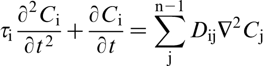
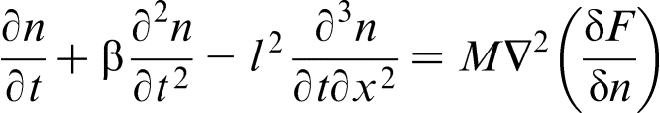
The next step to extend the hyperbolic PF and PFC models is to include the third order mixed derivative in the dynamical equations, which is responsible for space non-local effects.30,31,41–44 In such a case, the governing equation for the dimensionless local number density n (and concentration) can be rewritten as
Note that the conventional modelling of rapid solidification phenomena as well as PF and PFC approaches have used thermodynamic potentials to calculate the rate of non-equilibrium phase transformation. Although a non-zero free energy change means that there is a driving force for solidification, the rate of non-equilibrium phase transformation is not specified by the free energy change value. Strictly speaking, the rate is a kinetic parameter, which should be calculated from reaction rate theory.
Cellular automata and discrete heat mass transfer models
Cellular automata (CA) have been used to predict the interface evolution during binary alloy solidification due to their high computational efficiency.87–90 In particular, CA have been successfully combined with PF methods to predict the dendrite growth of multicomponent and multiphase alloys during the solidification process.
90
The microscale CA model was built to track the dendrite morphology evolution and associated variation of temperature–concentration fields, while PF model was used to calculate the growth kinetics. Cellular automata approach is analogous to the discrete heat mass transfer model, which introduces the discrete time τ and length h scales of the process and gives the transfer equations in the discrete form. According to its definition,30,41,91,92 the discrete model takes into account both time τ and space h non-locality of transfer processes and can be used directly in the discrete form as highly efficient tool for computer simulation. In the continuum limit  and
and  , the discrete model gives hierarchy of parabolic and hyperbolic continuum diffusion equations depending on the scaling law of the continuum limit.30,41,91,92 If
  and
and  so that
  has a finite value, then the continuum limit gives hierarchy of parabolic diffusion equations including classical diffusion equation as a first order approximation. The second order approximation gives the parabolic diffusion equation with two additional terms: second order time derivative and third order mixed derivative, which are responsible for the time and space non-local effects respectively. If
  and
and  so that
  has a finite value, then the continuum limit gives hierarchy of hyperbolic diffusion equations including HDE (equation (3)) as a first order approximation. The discrete model for the heat mass transfer processes can be also combined with MD, PF or PFC methods.
Conclusions
The local non-equilibrium diffusion effects play a decisive role in rapid alloy solidification: they lead to a sharp transition from diffusion controlled to diffusionless, thermal controlled solidification when the interface velocity V passes through the critical point  . The transition is accompanied by complete solute trapping and a sharp break of velocity–undercooling (or interface temperature–velocity) relationship. The local non-equilibrium diffusion effects and relevant phenomena, such as disorder and density trapping, grain refinement, absolute stability, etc., which have met substantial experimental difficulties in liquid–solid transformations, may be favourably investigated during solid state transformations and colloidal solidifications owing to the small diffusion coefficients and, hence, small diffusion velocities in such systems. The hybrid models, which combine the advantages of the continuum local non-equilibrium modelling with MD, PF and PFC methods, give us a new powerful tool to study real alloy solidification processes under extreme conditions. Molecular dynamics, PF and PFC methods can be used in the very phase transformation region, where active processes of phase transformations take place, whereas the continuum local non-equilibrium models are more efficient in a much wider region affected by the heat mass transfer in the system. The discrete heat mass transfer models and CA, which also take into account the local non-equilibrium effects, are particularly convenient for computer simulations because they do not need to be translated to the language of discrete mathematics and can be also used in combination with MD, PF and PFC methods.
Acknowledgements
The reported study was partially supported by RFBR, research project no. 14-48-03535.