Optimised recrystallisation model using multiobjective evolutionary and genetic algorithms and k -optimality approach

Abstract

The meta-models are constructed for static recrystallisation of dual phase steels using evolutionary neural nets (EvoNN). Four mutually conflicting objectives—(i) overall kinetics, (ii) grain size, (iii) the amount of strain and (iv) the precipitate volume fraction—are optimised simultaneously using an emerging k-optimal approach incorporated in the EvoNN, using a predator–prey genetic algorithm. The first objective involved minimisation of error with respect to experimental observation. The grain size and the amount of strain were minimised, whereas the precipitate volume fraction was maximised. The aim is to control the recrystallisation process in order to achieve desired material properties of dual phase steel during the final stages of heat treatment.

Keywords

Multiobjective optimisation Recrystallisation Genetic and evolutionary algorithms

Introduction

The data driven modelling has attracted enormous attention in recent times due to abundant supply of noisy data from various resources. The sources of data may vary from industry to scientific or engineering experiments and simulations, where the underlying physics of the process is often difficult to understand. Hence, the purpose of a data driven model is to construct a system model without directly referring to the underlying physics behind it, and at the same time, it attempts to efficiently capture any physical trend embedded in the data itself. In the current decade, multiobjective genetic algorithms based evolutionary neural net (EvoNN) algorithm proposed by Pettersson et al.¹ has efficiently performed the task of data driven modelling and optimisation for problems of diverse nature in the domain of materials design and processing.^2–9 Multiobjective evolutionary based machine learning processes are now quite established, as evident from some recent work^10–11; the application ranged from alloy design¹⁰ to machining and manufacturing.¹¹ In the recent past, a tree encoding based sister algorithm, known as bi-objective genetic programming (BioGP), has further augmented its scope.^12,13 The capability of genetic programming is already established in the metallurgical arena,¹⁴ and the advent of BioGP further augments it. Both EvoNN and BioGP are tuned to make intelligent models. These algorithms are capable of distinguishing between the essential and non-essential inputs, and use only the inputs that are deemed appropriate. In addition, they are capable of learning from the data trends the models that will lead to neither overfitting nor underfitting of the data.¹ Moreover, they are able to detect the trends of influence of each variable on the output.² Such features are not available in a traditional curve fitting exercise. These algorithms work quite efficiently in a situation where two objective functions are mutually conflicting and needed to be optimised simultaneously. However, in engineering or real world problems, the number of criteria to be optimised is often large, in which the abovementioned versions of EvoNN and BioGP cannot handle comfortably. The mathematical definition of Pareto optimality does not allow any objective of a candidate optimum solution to be inferior to the corresponding objective in another.^15–18 This is a very rigid requirement, quite difficult to implement in an evolutionary environment when the number of objectives is large. This leads to a problem in most multiobjective evolutionary algorithms, EvoNN and BioGP included. The remedy is to use some alternate less rigid optimal conditions.^19–21 One such option is to use the k-optimality condition recently proposed by Farina and Amato.²² The conditions implemented here allow a limited amount of inferiority in some of the objectives. It is thus more relaxed and less restrictive in terms of the possibility of locating the optimum solutions. The present study is an attempt to implement it in the context of a physical metallurgy problem related to the static recrystallisation of a dual phase (DP) steel. The study also incorporates other strategies like cellular automata and finite element method along with it. Further details are provided below.

Plan of action

The overall procedure of complete course of action is presented in Fig. 1. At first, the illustration based on different aspects of static recrystallisation (SRX) model is presented. Initially, a real microstructure is converted into digital form using digital material representation (DMR) technique. It is then incorporated into the SRX model. DMR provided the initial two-phase ferritic–pearlitic digital microstructure. This digital microstructure is then implemented into non-uniform finite element (FE) meshes to scale the macrobehaviour such as strain, temperature and stress of material in order to simulate the cold rolling process. Next part is the development of cellular automata (CA) model for processing SRX mechanism. The data collected from FE model are transferred into CA model using smoothed particle hydrodynamic (SPH) interpolation method in order to simulate the SRX process. The data obtained after simulating the complete SRX are incorporated into a data driven meta-modelling strategy in order to initiate the optimisation steps in the present investigation. During optimisation, the meta-models are formed by training the data set obtained from SRX model using evolutionary algorithm to capture the physical trends. Once the meta-models are formed, the optimisation task is performed using a modified predator–prey genetic algorithm (PPGA) described elsewhere.^1,4

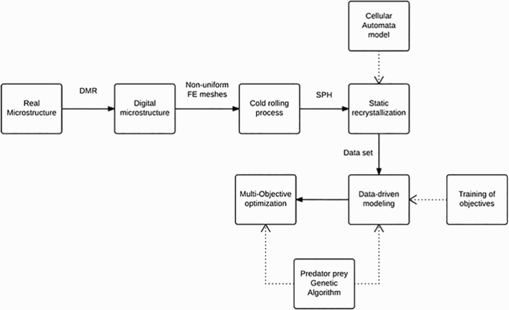
Flowchart describing different stages of overall process adopted

Further details of these computing methods and the associated concepts are briefly explained in the following section.

Concept adopted

Pareto optimality

Quite often in real world problems, situations arise where the objectives that need to be optimised are mutually conflicting to each other, i.e. none of the objectives will attain their individual best once an attempt is made to optimise them simultaneously. This leads to the situation of Pareto optimality, where a set of best possible tradeoffs between the objectives would constitute the optimum.²³ This notion of Pareto optimality does have a strong mathematical foundation²⁴ and forms the backbone of the data driven modelling as implemented in the present study.

Predator–prey genetic algorithm

The algorithm emulates the forest inhabitants such as predators and preys in a computational grid. The preys basically are the probable solutions for a given problem that need to be optimised, whereas the predators are computational entities, constructed to eliminate the weakest prey in their neighbourhood. Each computational grid may be occupied by either predator or prey, or it may be empty. A well defined hunting rule regulates the movement of both predator and prey. The predator moves to the grid occupied by the weakest prey after killing. The overall hunting process is terminated when the number of moves for all predators gets exhausted. Next, the breeding process starts with crossover and mutation. In crossover, two neighbouring solutions exchange few of their gene information and placed the children in any unoccupied grid randomly to achieve better gene pool mixing. In mutation, random alterations are made in gene values to obtain slightly different solution. The better individuals survive after prescribed generations are further screened through a ranking procedure to obtain the final Pareto tradeoffs.⁵ Evolutionary algorithms are far from a random search. The mathematics of this is very well established²⁵ and is beyond the scope of the present work.

Evolutionary neural nets

This algorithm applies PPGA to a population of neural networks of flexible topology and architecture.^1–9 Like the conventional artificial neural network, EvoNN also uses a lower layer, a hidden layer and an upper layer, but one striking difference is that it evolves optimally by computing a Pareto tradeoff between the network complexity and associated network training error. As explained in details earlier,¹ the number of weights in the lower layer of the network is taken as a measure of complexity in EvoNN. In BioGP, the same is defined as an average of the depth of the tree and the number of function nodes, as elaborated elsewhere.¹³ This is achieved by applying PPGA to a population of networks, and no separate training algorithm, for example, back propagation,²⁶ is used.

SRX model and k-optimality condition applied to recrystallisation

The ferrite recrystallisation is the initial stage in the manufacturing of DP steel, where new strain free grains are formed from previously deformed grains as a result of cold rolling process. Recrystallisation controls the overall mechanical and physical properties of DP steel. The size of new strain free grains is important for controlled nucleation and growth of austenite during intercritical annealing and also influences the cooling process. Earlier, a model called SRX model was proposed,²⁷ which could successfully simulate the recrystallisation process including cold rolling. The SRX model is complex in nature and associated with large number of process parameters. The optimisation of these process parameters is important in order to achieve desired properties of DP steel. The Pareto optimality condition¹⁵ that is conventionally applied in multiobjective problems is very difficult to implement through genetic and evolutionary algorithms, as a large number of solutions tend to become practically as good as each other and further improvements gets stalled. Hence, an alternative but less rigid optimal condition known as k-optimality proposed by Farina and Amato²² previously tested for a large number of objectives was implemented in EvoNN during this study in order to optimise the SRX model. The models created by the present strategies are well in accord with the standard Pearson's test. This is elaborated earlier³ and not repeated here. The details of SRX model and k-optimality condition are discussed below.

SRX model description

As stated before, the SRX process starts with the implementation of real microstructure into digital format using DMR technique.²⁸ DMR converts the real microstructure into digital material model via image processing algorithm to exactly replicate the complex detailing like different phases and different grains. This technique is very useful for detailed virtual analysis of microstructure. DMR provides the initial two-phase ferritic–pearlitic digital microstructure for performing cold rolling and recrystallisation processes. Next, the digital microstructure is incorporated into non-uniform FE meshes in order to capture the material behaviour. A diversification in the flow curves is applied to each grain due to different crystallographic orientation using introduction of Gaussian distribution. Hence, each adjacent grain differs slightly by flow stress values. The macroscale behaviour of material is modelled here by providing the information about general strain, stress, temperature in macroscale level and microstructural behaviour in microscale level in the FE meshes. At first, macroscale simulation is carried out for cold rolling process, and after that, microscale information are collected on the basis of macroscale simulation. Numerical simulation results of cold rolling process are obtained using this procedure.²⁷ Next part is the development of CA model for SRX. 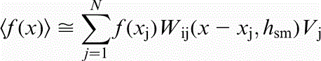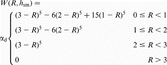First, data from FE model are transferred into CA model using SPH interpolation method.²⁹ The value of integral representation of function at location x is known in a finite set of discrete point, and then it can be written as follows: (1) where is the kernel approximation, is the kernel function, is the smoothing length, and is the volume of the j th particle. The value of function at point x is calculated by adding all the contributions from set of neighbouring j particles from support domain of x particle. The kernel function should meet certain consistency conditions in order to become applicable in SPH method. Out of several forms, the present work is using quintic spline kernel function. (2) where

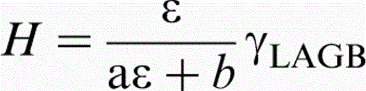
After successful interpolation and transfer of data into CA computational space, the strain field is converted into accumulated energy. (3) is the equivalent strain, a and b are the coefficients, and is the energy of low angle grain boundary.

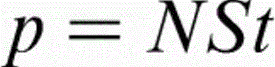
All the obtained data serve as the input for the simulation of CA-SRX model. The model is created in two-dimensional spaces with 2114 × 183 cells, where each cell equaled 0.229 μm with respect to physical dimension. The cells resembled either of the two states: recrystallised or unrecrystallised. In case of unrecrystallised cell state, the probability of formation of recrystallised nuclei is determined by (4) where S is the volume in which nucleus appeared, t is the time, and N is the coefficient.

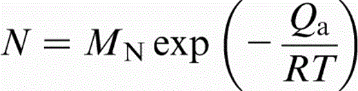
The coefficient N is computed by Arrhenius equation type: (5) where is the activation energy for nucleation, R is the universal gas constant, T is the temperature, and is another coefficient that is computed based on equation: (6) where is the parameter related with scaling, is the energy in the cell, and is the critical energy required for nucleation.

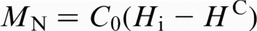
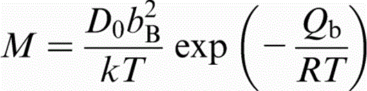
Once the nuclei appeared in the microstructure, grain growth process starts. Two major factors are controlling the growth process of recrystallisation: stored energy and grain boundary curvature. The latter was calculated as: (7) where P is the net pressure on grain boundary and M is the mobility factor of grain boundary that is calculated as: (8) where is the diffusion constant, is the Burger's vector, k is the Boltzmann's constant, and is the activation energy of grain boundary movement.

Hence, during simulation of SRX, the above procedure incorporates the cold deformed strain induced two-phase microstructure that occurs in this system.

k-optimality condition

The definition of Pareto optimality states that any solution in feasible space is considered better only if it is at least as good as any other solution in terms of all the objectives and strictly better in terms of at least one objective. This Pareto condition becomes restrictive when the objectives are large, as the number of solutions that satisfy this condition becomes small. Hence, an alternative strategy, known as k-optimality condition,²² is implemented here. In this version of optimality, any objective in a candidate solution can be better, equivalent or worse compared to the corresponding objective in another. Thus, a candidate solution for k-optimality, when considered in terms of all the objectives, can be assigned any of these three possible states to its constituent objectives, while in Pareto criteria, only better and equivalent solutions are considered. As for example, suppose there are 10 objectives, if a candidate solution is the same for six objectives when compared with second solution, then, in order to dominate the second solution, the first solution must be strictly better in the remaining four objectives. Hence, in Pareto's condition, there is no room for a worse performance in terms of any of the objectives. A worse performance, however, is possible to accommodate in k-optimality, as illustrated below.

If and are two candidate solutions in feasible domain space Ω so that . Three different functions , and take into account the number of objectives M for which solution is better, equivalent and worse respectively as compared to solution . According to the definition of k-optimality, solution is considered better than solution , if and only if the following conditions are satisfied: (9) (10) Hence, for k = 1, , in principle, even half of the feasible solutions could be inferior. For k = 0, we get back the original Pareto optimality condition. Generally, the larger the number of objectives, the higher could be the chosen k value.

Problem formulation

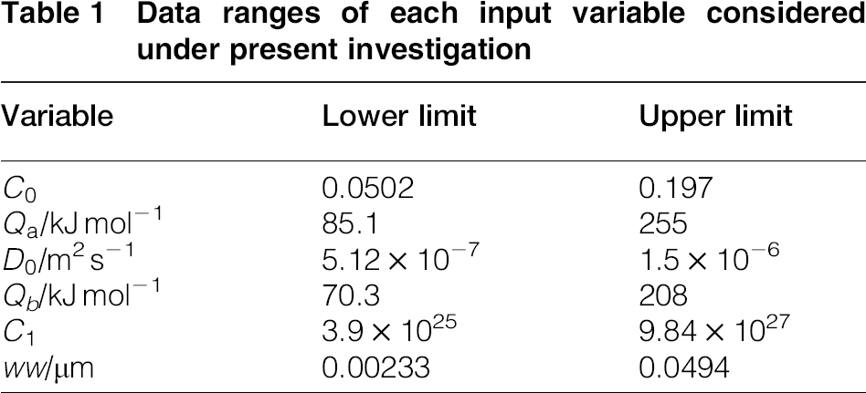
Many variables are used for the simulation of SRX process. In the present study, four parameters have been identified as important for the optimisation task using meta-modelling technique. These parameters are as follows: overall kinetics of the recrystallisation process with respect to experimental observation, grain size after SRX, amount of strain during SRX process and precipitate volume fraction. The first parameter tracks the difference in kinetics of recrystallisation predicted by the model with respect to experimental observation. By optimising first objective, one can obtain an accurate prediction of recrystallisation process. The second objective, grain size, is very essential for good mechanical as well as for physical properties of steel. As the recrystallised grain size decreases, the grain boundaries increase and act as the favourable nucleation sites of austenite during intercritical annealing. The overall grain refinement is enhanced when the recrytallised grains are small. The third objective, the amount of strain during recrystallisation process, determines whether the static or dynamic recrystallisation process occurs. If the strain crosses a critical limit, then the SRX is replaced by dynamic recrystallisation. The SRX model, as the name suggests, is modelled for SRX process. Hence, if strain value crosses the critical limit, then the overall calculations become wrong. The fourth parameter, precipitate volume fraction, directly controls the grain size during recrystallisation process by arresting the movement of grain boundary. Hence, these four parameters are selected for optimisation using k-optimality code. The input variables that control all these objectives are as follows: , scaling parameter during nucleation; , activation energy for nucleation; , diffusion constant; , activation energy of grain boundary movement; , scaling parameter to estimate the influence of recovery; ww, particle radius of precipitate under consideration of Zener pinning effect.³⁰ The data range of the input variables used for present investigation is shown in Table 1.

Table 1

Data ranges of each input variable considered under present investigation

Variable	Lower limit	Upper limit
	0.0502	0.197
/kJ mol^− 1	85.1	255
/m² s^− 1	5.12 × 10^− 7	1.5 × 10^− 6
Q_b/kJ mol^− 1	70.3	208
	3.9 × 10²⁵	9.84 × 10²⁷
ww/μm	0.00233	0.0494

This study, in view of the above discussions, required simultaneous optimisation of four objectives as listed below: 1

Optimise overall kinetics of recrystallisation (minimise the error between predicted model kinetics and experimental observation)

Minimise recrystallised grain size

Minimise amount of strain

Maximise precipitate volume fraction.

A total of ∼450 data entries were collected for the optimisation task. The meta-models were created to optimise the four selected objectives. In the first part, all the 450 data entries were trained using the EvoNN. It intelligently learned the different data patterns by avoiding the outliers and noises present inside the data entries. Each objective was trained individually with the same set of input variables. The training was ran for 300 generations where other genetic algorithms parameters like lattice size, predator population, prey population, kill interval and number of nodes were set at 50, 200, 500, 20 and 10 respectively. In the next step, all those trained models were optimised at different k values. The k values were varied from 0 to 1 with 0.25 interval gap. Therefore, the five different k values selected were 0, 0.25, 0.5, 0.75 and 1. While running the k-optimisation algorithm, some target values were first set for individual objectives, and later, the error was minimised with respect to those target values. The minimum values for F1, F2 and F3 in data ranges were 2.21, 0.8 μm and 0.1, whereas the maximum value of F4 in the data set was 2.99 volume fraction. Based upon these, the target values for four objectives were chosen as 0, 0, 0.1 and 3 respectively. The purpose of this task is to set the target that matches with the minimum or maximum limit of the data ranges in order to achieve the minimisation or maximisation task respectively. On the other side, slightly modified form of PPGA was implemented in k-optimality algorithm. In the modified version, the criterion of killing preys was modified. Here, it was achieved using highest k-dominance factor instead of worst fitness evaluated around the predators. In the modified version of k-optimality algorithm, the mutation was taking single probability value of 0.1 instead of randomly chosen one- and two-point crossovers with probability of 0.95 set in the algorithm.

Results and discussion

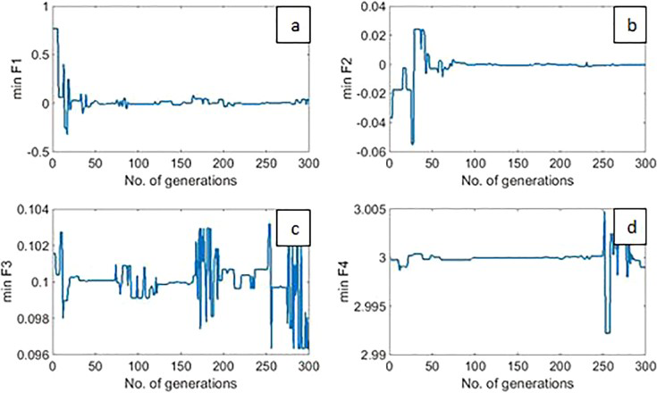
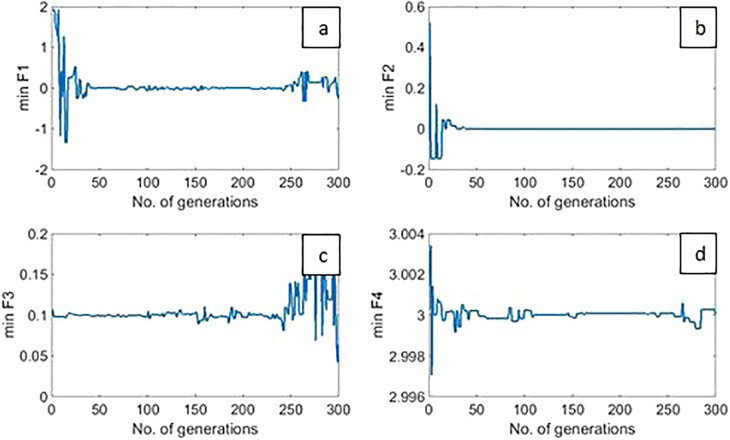
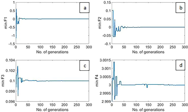
The k-optimal fronts at different k values are shown in Fig. 2a– e . At k = 0, it indicates the real Pareto optimality. In Fig. 2, the x axis represents the number of generations for which the code was running and y axis indicates different objectives. Here, F1, F2, F3 and F4 in y axes are overall kinetics, grain size, amount of strain and precipitate volume fraction respectively. The first three objective functions F1, F2 and F3 have been minimised, whereas F4 has been maximised. Figure 2 shows the best solutions that are closest to the target values at each generation.

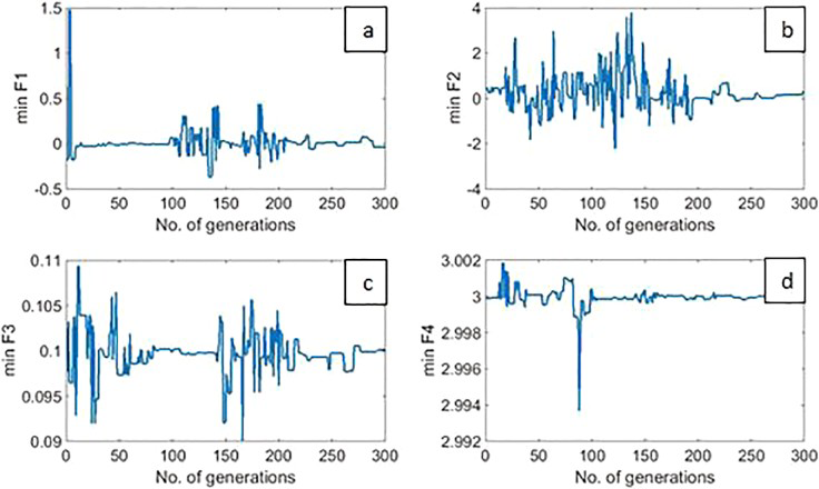
Optimised results at k = 0 after 300 generations for objectives a overall kinetics, b recrystallised grain size, c strain and d precipitate volume fraction

Optimised results at k = 0.25 after 300 generations for objectives a overall kinetics, b recrystallised grain size, c strain and d precipitate volume fraction

Optimised results at k = 0.5 after 300 generations for objectives a overall kinetics, b recrystallised grain size, c strain and d precipitate volume fraction

Optimised results at k = 0.75 after 300 generations for objectives a overall kinetics, b recrystallised grain size, c strain and d precipitate volume fraction

Optimised results at k = 1 after 300 generations for objectives a overall kinetics, b recrystallised grain size, c strain and d precipitate volume fraction

The objective F1 is related with the overall kinetics of phase transformation during recrystallisation process. The initial part of conventional S shape kinetics curve is associated with the nucleation that is followed by growth at constant rate in the middle period and the effect of impingement sets in and at the final stage when the process of growth slows down. In Fig. 2a– e , for all k values, a close approximation of the kinetics of transformations is achieved with respect to experimental observation. It implies that the closer the approximation with experiments, the more exact nucleation in terms of number and time was activated during the recrystallisation process. This effect leads to small grain size due to formation of large number of recrystallised nuclei. The SRX model considered SRX, where nucleation and growth only occurred during the heat treatment process. Hence, the amount of strain F3 should be lower enough to hinder the occurrence of nucleation and growth during deformation via the cold rolling process. The target of objective F3 was best achieved in case of k equals to 0, 0.25 and 1. The objective F4 arrested the movement of grain boundary during growth of recrystallised nuclei and that helps to achieve small grain size. The maximum limit for F4 was set at 3 of total volume fraction, and it was achieved in most cases of k values. The input variables like activation energy for grain boundary movement, diffusion coefficient, precipitate particle radius and activation energy for nucleation are playing important roles in order to achieve such good optimised results. The activation energy for nucleation is the rate determining step of recrystallisation and should be higher. The lower diffusion constant is anticipated, as the movement through the grain boundary is faster compared to bulk due to the presence of large defects. The precipitate particle size influences the objective F2 more profoundly. The larger size would help to restrict the grain boundary movement. The activation energy for grain boundary movement is an important aspect to control the overall objectives. The grain boundary motion is greatly influenced by the effect of recovery, strain heterogeneity, precipitate particle size and precipitate volume fraction. Lower activation energy during boundary motion would help to maintain the balance. More detailed analysis is provided later to understand the exact behaviour of each input variables.

In Fig. 2a– e , apart from initial inconsistency, the algorithm made adjustment accordingly to find the optimum, where all the objectives are converged and further improvement is not possible. Figure 3 provided the information of overall root mean square error (RMSE) of each k value selected for investigation. The least RMSE in case of all k values is calculated by adding the individual RMSE of four objectives. The other interesting information in Fig. 3 is that the RMSE values at k equals to 0 and 0.25 are not smooth enough, whereas the RMSE values for the remaining three k values are smooth and linearly improve the solutions.

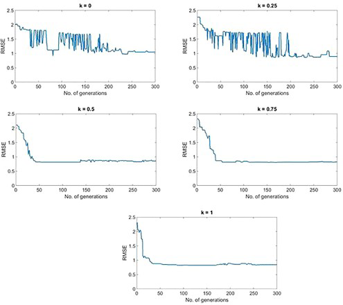
RMSE obtained for 300 generations in case of five different k values

The generation at which the least RMSE is calculated for each k value is shown in Fig. 4. The least RMSE values are calculated by analysing the result presented in Fig. 3. The least RMSE for 0 k value was found at 81st generation, and the value was ∼0.91269. Similarly, for k values 0.25, 0.5, 0.75 and 1, the least RMSE of 0.85766, 0.8145, 0.80928 and 0.82037 was found at 160th, 97th, 113th and 110th generations respectively. The RMSE of 0.80928 for k = 0.75 is the lowest among all the values and hence considered the best k. The reason for such behaviour is obvious since the relaxation in dominance criteria (in terms of increasing k value) increases the chances of survival for more optimum solutions, which finally provided the better solutions. This comparison indicated that the Pareto's optimal condition is not sufficient when the number of criteria to be optimised is high.

Plot of least error found at different k values and particular generations

Further, the values are analysed for solution that showed least RMSE for k = 0.75 at 113th generations. The values of both input and output variables are the following. The best solution showed Y1, Y2, Y3 and Y4 as 0.071418, 0.007829 μm, 0.191784 and 0.036761 percent of total volume respectively. All the output results are quite close to target value except the fourth variable, where the difference is enormous. Similarly, for best solution, the input variables X1, X2, X3, X4, X5 and X6 are 0.1568, 192.3380 kJ mol^− 1, 5.18 × 10^− 7m² s^− 1, 75.43 kJ mol^− 1, 9.2 × 10²⁷ and 0.0309 μm respectively. When the individual input variables are compared with the lower and upper limit of the range provided in Table 1, then the physical trend of the input variables can be analysed. The trend is like that—the values for X1, X2, X5 and X6 are found to be on the higher side and the rest showed the values on the lower side. The same results are analysed for the second best solution for k = 0.5 at 97th generation and found that the trend is similar. Hence, for better result, the values of input variables , , and ww need to be on the higher side, whereas the values related with diffusion constant and activation energy for grain boundary movement need to be on the lower side. This behaviour of input variable exactly matches the expectation as mentioned above.

The literature indicated that the activation energy of grain boundary motion is ∼140–150 kJ mol^− 1.^31,32 The current analyses of the optimised results reported the activation energy of 75.43 kJ mol^− 1. The deformation considered in the present investigation during cold rolling is ∼50–70, which is high enough to generate large dislocation density. The driving force for grain boundary motion is dependent on the density of defects, e.g. dislocation. An excess density of defects in the growing grain boundary is a powerful source of driving force for faster diffusion of growing atom as compared to regular lattice diffusion. On the other hand, the precipitate of 0.036761 of total volume in case of optimised results is achieved, which exerts very little solute drag effect to hinder the movement of growing grain boundary. In addition, the solute drag effect is significant when there is some interaction energy between boundary and second phase particle in order to segregate in grain boundaries, and to some extent, it depends on the position of the second phase particles. All these effects resulted into low activation energy of grain boundary movement. The other parameter, activation energy for nucleation in case of optimised results, is in the vicinity of the literature values. For deformation inhomogeneities where the concentration of defects is large, stored energy is high and it restricts the movement of interfaces. This condition promotes the formation of new stable phase (heterogeneous nucleation) with less stored energy due to annihilation of dislocations. However, in the present model, homogeneous nucleation is also considered, which possesses higher activation barrier. Therefore, the optimised results reported a mid-range value of 192 kJ mol^− 1 as compared to 170 kJ mol^− 1 reported in the literature. Although, for exerting pinning effect, many criteria like position and volume fraction of second phase particle are important, the size of precipitate particle is, however, the most important factor in order to arrest the movement of grain boundaries. When the size of precipitate particle crosses the critical mean radius, then it exerts maximum force to restrict the motion of boundaries. As expected, the optimum points from the obtained result show a trend towards the higher side of particle size in the data set.

Conclusions

The present study successfully optimises four objectives simultaneously obtained from SRX model of DP steels using a less restrictive k-optimality condition incorporated in the modified EvoNN algorithm. The k values of 0, 0.25, 0.5, 0.75 and 1 were selected for the present investigation to optimise four objectives simultaneously: (i) optimum overall kinetics of recrystallisation, (ii) minimise recrystallised grain size, (iii) minimise the amount of strain and (iv) maximise the precipitate volume fraction. The optimisation runs for 300 generations. The best solution was obtained for the k value of 0.75 at 113th generation, evaluated by adding the RMSE values of the individual objectives. Expectedly, the worst solutions were obtained at k = 0, which corresponds to Pareto condition, as true Pareto optimality could not be generated in the presence of four objectives. By analysing the best solutions at each k values, the optimum was obtained when the input parameters such as activation energy of grain boundary movement and diffusion constant were low and the remaining input parameters were high. The optimum achieved for individual input parameter ensures that the kinetics of model is in close approximation with the experimental results, and minimum recrystallised grain size, minimum strain value and appropriate precipitate volume fraction are obtained to provide desired macro- and microproperties for intercritical annealing during austenite transformation that will affect the final material properties of DP steels.

References

Pettersson

, Chakraborti

and Saxen

: ‘A genetic algorithms based multi-objective neural net applied to noisy blast furnace data’, Appl. Soft Comput., 2007, 7, 387–397. doi: 10.1016/j.asoc.2005.09.001

Mohanty

, Cahndra

and Chakraborti

: ‘Genetic algorithms based multi-objective optimization of an iron making rotary kiln’, Comp. Mater. Sci., 2009, 45, 181–188. doi: 10.1016/j.commatsci.2008.03.056

Jha

, Sen

P. K.

and Chakraborti

: ‘Multi-objective genetic algorithms and genetic programming models for minimizing input carbon rates in a blast furnace compared with a conventional analytic approach’, Steel Res. Int., 2014, 85, (12), 219–232. doi: 10.1002/srin.201300074

Mondal

D. N.

, Sarangi

, Pettersson

, Sen

P. K.

, Saxen

and Chakraborti

: ‘Cu–Zn separation by supported liquid membrane analyzed through multi-objective genetic algorithms’, Hydrometallurgy, 2011, 107, 112–123. doi: 10.1016/j.hydromet.2011.02.008

Halder

, Madej

, Pietrzyk

and Chakraborti

: ‘Optimization of cellular automata model for the heating of dual phase steel by genetic algorithm and genetic programming’, Mater. Manuf. Process., 2015, 30, 552–562. doi: 10.1080/10426914.2014.994765

Rajak

, Tewary

, Das

, Bhattacharya

and Chakraborti

: ‘Phases in Zn-coated Fe analyzed through an evolutionary meta-model and multi-objective genetic algorithms’, Comp. Mater. Sci., 2011, 50, 2502–2516. doi: 10.1016/j.commatsci.2011.03.034

Rajak

, Ghosh

, Bhattacharya

and Chakraborti

: ‘Pareto-optimal analysis of Zn-coated Fe in the presence of dislocations using genetic algorithms’, Comp. Mater. Sci., 2012, 62, 266–271. doi: 10.1016/j.commatsci.2012.05.002

Hariharan

, Nguyen

N. T.

, Chakraborti

, Lee

M. G.

and Barlat

: ‘Multi-objective genetic algorithms to optimize variable drawbead geometry for tailor welded blanks made of dissimilar steels’, Steel Res. Int., 2014, 85, 1597–1607. doi: 10.1002/srin.201300471

Hariharan

, Chakraborti

, Barlat

and Lee

M. G.

: ‘A novel multi-objective genetic algorithms-based calculation of Hill's coefficients’, Metall. Mater. Trans. A, 2014, 45A, 2704–2707. doi: 10.1007/s11661-014-2274-5

10.

Arisoy

Y. M.

and Ozel

: ‘Machine learning based predictive modeling of machining induced microhardness and grain size in Ti–6Al–4V alloy’, Mater. Manuf. Process., 2015, 30, 425–433. doi: 10.1080/10426914.2014.961476

11.

Jha

, Pettersson

, Dulikravich

G. S.

, Saxen

and Chakraborti

: ‘Evolutionary design of nickel-based superalloys using data-driven genetic algorithms and related strategies’, Mater. Manuf. Process., 2015, 30, 488–510. doi: 10.1080/10426914.2014.984203

12.

Giri

B. K.

, Hakanen

, Miettinen

and Chakraborti

: ‘Genetic programming through bi-objective genetic algorithms with a study of a simulated moving bed process involving multiple objectives’, Appl. Soft Comput., 2013, (5), 2613–2623. doi: 10.1016/j.asoc.2012.11.025

13.

Giri

B. K.

, Pettersson

, Saxen

and Chakraborti

: ‘Genetic programming evolved through Bi-objective genetic algorithms applied to a blast furnace’, Mater. Manuf. Process., 2013, (7), 776–782. doi: 10.1080/10426914.2013.763953

14.

Kovacic

: ‘Modeling of total decarburization of spring steel with genetic programming’, Mater. Manuf. Process., 2015, 30, 434–443. doi: 10.1080/10426914.2014.961477

15.

Chakraborti:

: ‘Critical assessment 3: the unique contribution of multi-objective evolutionary and genetic algorithms in materials research’, Mater. Sci. Technol., 2014, 30, 1259–1262. doi: 10.1179/1743284714Y.0000000578

16.

Chakraborti

: ‘Promise of multiobjective genetic algorithms in coating performance formulation’, Surf. Eng., 2014, 30, 79–82. doi: 10.1179/1743294413Y.0000000219

17.

Chakraborti

: ‘Evolutionary data-driven modeling—informatics for materials science and engineering’ 71, ; 2013, Oxford, Butterworth-Heinemann.

18.

Chakraborti

: ‘Strategies for evolutionary data-driven modeling in chemical and metallurgical systems—applications of metaheuristics in process engineering’ 89, ; 2014, Basel, Springer.

19.

Adeyemo

J. A.

and Olofintoye

O. O.

: ‘Evaluation of combined Pareto multiobjective differential evolution on tuneable problems’, Int. J. Simul. Model., 2014, 13, (3), 276–287. doi: 10.2507/IJSIMM13(3)2.264

20.

Coello

C. A. C.

and Becerra

R. L.

: ‘Evolutionary multiobjective optimization in materials science and engineering’, Mater. Manuf. Process., 2009, 24, (2), 119–129. doi: 10.1080/10426910802609110

21.

Zhou

, Qu

B. -Y.

, Li

, Zhao

S. -Z.

, Suganthan

P. N.

and Zhang

: ‘Multiobjective evolutionary algorithms: a survey of the state of the art’, Swarm Evolut. Comput., 2011, 1, (1), 32–49. doi: 10.1016/j.swevo.2011.03.001

22.

Farina

and Amato

: ‘On the optimal solution definition for many-criteria optimization problems’. Proc. Int. Conf. on ‘NAFIPS-FLINT International Conference’, Piscataway, NJ, IEEE Service Center, June 2002, 233–238.

23.

Deb

: ‘Multi-objective optimization using evolutionary algorithms’, 30–34; 2001, New York, Wiley.

24.

Steponavice

, Ruuska

and Miettinen

: ‘A solution process for simulation-based multiobjective design optimization with an application in the paper industry’, Comput. Aided Design, 2014, 47, 45–58. doi: 10.1016/j.cad.2013.08.045

25.

Vose

M. D.

: ‘The simple genetic algorithm: foundations and theory’; 1999, Cambridge, MA, MIT Press.

26.

Wang

, Zeng

and Chen

: ‘Back propagation neural network with adaptive differential evolution algorithm for time series forecasting’, Expert Syst. Appl., 2015, 42, 855–863. doi: 10.1016/j.eswa.2014.08.018

27.

Madej

, Sieradzki

, Sitko

, Perzynski

, Radwanski

and Kuziak

: ‘Multi scale cellular automata and finite element based model for cold deformation and annealing of a ferritic–pearlitic microstructure’, Comp. Mater. Sci., 2013, 77, 172–181. doi: 10.1016/j.commatsci.2013.04.020

28.

Madej

, Wang

, Perzynski

and Hodgson

P. D.

: ‘Numerical modeling of dual phase microstructure behaviour under deformation conditions on the basis of digital material representation’, Comp. Mater. Sci., 2014, 95, 651–662. doi: 10.1016/j.commatsci.2014.08.035

29.

Longshaw

S. M.

and Rogers

B. D.

: ‘Automotive fuel cell sloshing under temporally and spatially varying high acceleration using GPU-based smoothed particle hydrodynamics (SPH)’, Adv. Eng. Softw., 2015, 83, 31–44. doi: 10.1016/j.advengsoft.2015.01.008

30.

Moidownik

M. A.

: ‘Zener pinning’, 2nd edn, ‘Encyclopedia of materials: science and technology’, 9855–9859; 2001, New York, Elsevier.

31.

Zheng

, Xiao

, Li

and Li

: ‘Microstructure prediction of the austenite recrystallization during multi-pass steel strip hot rolling: a cellular automaton modeling’, Comp. Mater. Sci., 2008, 44, 507–514. doi: 10.1016/j.commatsci.2008.04.010

32.

Yang

B. J.

, Chuzhoy

and Johnson

M. L.

: ‘Modeling of reaustenitization of hypoeutectoid steels with cellular automaton method’, Comp. Mater. Sci., 2007, 41, 186–194. doi: 10.1016/j.commatsci.2007.04.001