Digital image correlation for grain scale strain measurement in interstitial free high strength steel

Abstract

Deformation measurement of materials and structures subjected to various loading conditions is an important task of experimental solid mechanics. Apart from the widely used point wise strain gauge technique, various full field non-contact optical methods are used for this purpose. In this work, an automated scheme to measure the grain level deformation in tensile deformed interstitial free high strength steel has been introduced. The method is based on digital image correlation technique. The proposed scheme utilised high resolution scanning electron images of the specimen surface that are sequentially captured during tensile loading. It is found that grain to grain there is large variation in deformation response at a given load. The present work also reveals point to point variation of strain within a grain interior.

Keywords

Image correlation Strain measurement Grain segmentation Micrograph processing IFHS steel

Introduction

Deformation measurement of materials and structures subjected to various loading conditions (mechanical or thermal) is an important task of experimental solid mechanics. The deformation behaviour of different materials under load that are routinely studied is an average response of the microstructure of a material. It is by now established and well documented in the literature that plastic deformation in polycrystalline materials is never homogeneous, whether the material consists of a single phase or multiple phases. Orientation difference of individual grain with respect to the loading axis is responsible for grain to grain variation in plastic deformation even when deformation is macroscopically homogeneous.^1–3 Further, deformation heterogeneity also exists within individual grain. Raabe et al.⁴ have elaborately discussed the occurrence of deformation heterogeneity within individual grain in coarse grained aluminium specimen. In order to know the influence of different grains and other phases constituting the material's microstructure, sophisticated experimental and finite element modeling techniques are often used. Nowadays, electron back scatter diffraction technique in conjunction with scanning electron microscopy (SEM) is being exploited to understand the deformation heterogeneity in polycrystalline materials. Deformation experiments directly under SEM also provide scope for studying the deformation response of individual grain under load. In this technique, the grain structure and other constituting phases of the material are directly observed during deformation. It is known that the deformation characteristic of individual grain depends on its crystallographic orientation and also on the orientation of the surrounding grains with respect to loading axis. Collectively, the deformation of individual grain controls the average deformation behaviour of a material. As a result, investigation towards understanding the nature of microlevel deformation has gained impetus over the last few years.^5–11 It is worth mentioning that strain measurements at any point in an area of interest are required for better understanding of the deformation behaviour of materials and structural components. For this reason, researchers are interested on a strain map over a specimen surface. Use of digital image processing techniques has enabled such measurements.

Digital image correlation (DIC) is an optical method that uses a mathematical correlation analysis to examine digital image data taken while the specimens are subjected to incremental load. As discussed and reviewed by Qian et al.¹², two-dimensional DIC is a practical and effective tool for quantitative in-plane deformation measurement of a planar surface, and it is widely accepted where contact method of strain measurement is difficult. Measurement of small difference in the images supports such correlation.¹³ Electronic speckle photography offers a simple and fast technique for measuring in plane displacement fields in solid and fluid mechanics. An improved algorithm for measuring the correlation between subimages has been presented by Sjodahl.¹⁴ The Vic2D presented by Cintron et al.¹⁵ is an innovative approach that uses the DIC technique for strain measurements in a two-dimensional contour map of planar surfaces. But it cannot provide displacement and strain maps after the specimens show cracks because of poor correlation. The maps obtained from the specimen images that show cracks are not adequate to determine the strain values at some locations inside the area of interest. It is also reported that the DIC technique can also used to determine the heterogeneity and severity of deformation in polycrystals.¹⁶ Besides, in situations where it is difficult to measure the strain directly, this technique finds application in knowing macroscopic strain during creep deformation.¹⁷

A novel microscopic strain mapping technique based on DIC has been developed in recent years for various applications in materials characterisation. In these cases, input is a series of SEM images, and strain mapping is done based on the topographic features of the images. For this purpose, many researchers^18,19 use commercially available optical strain measurement system (ARAMIS), which utilises the DIC methodology. Cao et al.²⁰ have proposed a simple and efficient non-contact method to overcome the difficulties of determining Poisson's ratio using traditional contact method. They used DIC method in their work and obtained the relative deformation of specimens using calibrated CCD images.

Interstitial free high strength (IFHS) steels of 1 to 2 mm thickness find extensive applications in automotive industries for their very good cold formability and reasonable strength properties. Volumes of work have already been done correlating processing parameters with the development of texture that controls the formability of the steel. Our interest is, however, different, and we focused our attention to develop an automated methodology for knowing the deformation pattern of individual grain when a specimen made of 1 mm thick IFHS steel is subjected to incremental load. The impetus for developing such automated methodology stems from the fact that the commercial DIC software that is used to know the local strain distribution using the images as an input works as a black box. This automated methodology has been developed by employing image analysis procedure on scanning electron micrographs captured during deformation.

Experimental

The IFHS steel sheet of 1 mm thickness received from TATA Steel, Jamshedpur, India, has been used in the present investigation. The chemistry of the steel in wt. pct is: Fe–0.0029C–0.39Mn–0.004Si–0.007S–0.05P–0.005Si–0.018Cr–0.044Al – 0.005Cu – 0.001Nb – 0.042Ti–0.0018N. Optical microscopy reveals that the microstructure of the steel consists of polyhedral grains of ferrite, as shown in Fig. 1. The two-dimensional average grain size of the steel is about ASTM 10. Tensile properties of the steel deformed at a strain rate of 10^− 3 sec^− 1 are: Y.S = 189 MPa, T.S = 374 MPa, Uniform elongation = 21 pct, Total elongation = 37 pct.

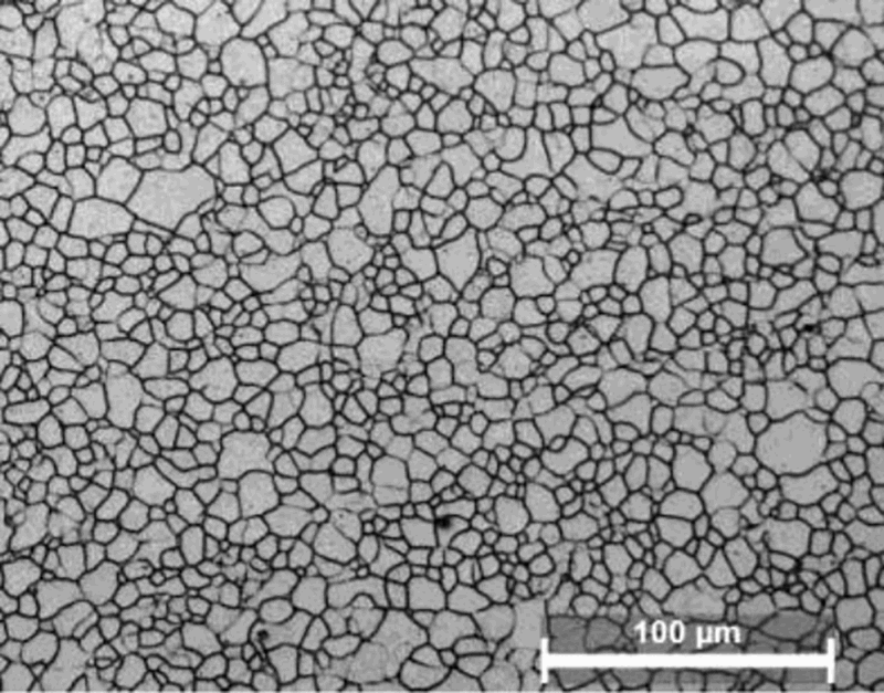
Optical microstructure of investigated IFHS steel

Tensile deformation experiments were also done directly under SEM using miniature sized tensile specimen fabricated by wire electrodischarge machining process while keeping the specimen axis parallel to the rolling direction. One surface of the specimen was metallographically polished in successive steps, and final polishing has been done using 1 μm diamond paste. The polished specimen has been thoroughly cleaned, dried and then etched with Marshall's reagent in order to reveal the grains lying on the surface. The polished and etched specimen has been deformed under tensile loading at a deformation rate of 1 mm per minute inside the vacuum chamber of an SEM (FEI, Quanta 450). The loading device was screw driven GATAN, UK make tensile/bending deformation stage.

It should be noted here that from a number of trial experiments, we observed that the pin loading arrangement of the tensile deformation stage that we used in the present investigation does not accurately measure the specimen strain because of slackness of the loading arrangement, particularly at the low load level. To overcome this difficulty, we measured the specimen strain between two collinear microindentation marks separated by 2000 μm put on the polished and etched specimen surface placed before the deformation experiment. The specimen was then loaded in steps, and high resolution secondary scanning electron images were captured after each step of loading. The strain measured within these two microindentation marks is termed here as global strain. Thus, a series of scanning electron micrographs were obtained until complete fracture of the specimen. These images were subsequently processed to find the grain level deformation pattern. Here, the image in the undeformed condition is called as reference image, and image correlations have been done with respect to this undeformed image to find the grain level deformation. Figure 2 shows a sequence of secondary scanning electron images corresponding to different load levels. The present study is based on these images. The stress and strain corresponding to the images are shown in Table 1.

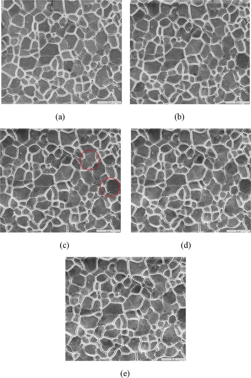
Sequence of secondary scanning electron images at different loads

Table 1

Global stress–strain behaviour corresponding to captured micrographs

Micrographs	Stress/MPa	Strain measured experimentally/
Micrograph 1 (Fig. 2a)	0	0.00
Micrograph 2 (Fig. 2b)	116	1.14
Micrograph 3 (Fig. 2c)	174	2.56
Micrograph 4 (Fig. 2d)	233	6.00
Micrograph 5 (Fig. 2e)	282	8.26

Proposed methodology for evaluating grain strain

In general, a micrograph reveals the size, shape and distribution of different constituting phases or grains. During deformation of the specimen, grain shape is changed depending upon its size, crystallographic orientation and load level. Additionally, deformation features, for example, slip lines, also become visible in the high resolution scanning electron micrographs of the deformed specimen. However, crystallographic orientation of the grains with respect to loading axis has not been considered in the present work. The major steps involved in the present study are grain segmentation, tracking the grains in the sequentially captured micrographs and grain level strain measurement. It should be noted here that in the present study the estimation of grain level strain has been done only in the loading direction, that is along the tensile axis, which coincides with the horizontal direction of every image frame.

Grain segmentation

Image segmentation refers to the automatic extraction of the regions of interest from the image. Ideally, a region should be homogeneous in terms of a certain property that characterises the region. Identifying such property is an important task in the segmentation process. A closed boundary separates the segmented region from the rest. One common approach of segmentation is to detect the boundary. Since our aim is to develop an automated process for studying the grain level strain distribution, it becomes necessary to extract the individual grain present in a micrograph.

A sample micrograph composed of a number of grains is shown in Fig. 3a. It is observed that a grain is normally enclosed within a boundary that separates it from the adjoining grains. It is also observed that mostly the grains consist of pixels with low intensity values. On the contrary, the boundary pixels are of high intensity values. Our motivation is to detect the closed (without any break/discontinuity) boundary encompassing a grain. However, a simple intensity based threshold technique does not always serve the purpose. There may be weak boundaries with not so high intensity value. Again, different grains may have different intensity levels even though a grain is more or less uniform in terms intensity. Thus, it is possible to have an overlap between the intensity values of the pixels inside the grains and those in the boundaries. As a result, some pixels in the grain may be incorrectly marked as boundary. On the other hand, part of the boundary (weak portions) may be missed out and will give rise to discontinuity. Thus, obtaining the desired closed contours that enclose the grain is a major challenge. Furthermore, the selection of proper intensity value as the threshold is also very difficult. Therefore, a suitable property of the image other than the intensity value is to be explored for segmentation purpose. Careful observation of the micrographs reveals that contrast can act as a suitable property in the segmentation problem under consideration. Contrast stands for the difference in intensity values between two regions in the image. The grain boundary in the micrograph becomes visible provided there is a perceivable change in contrast between the boundary and the grain interior. With these observations, we look forward to adopt a suitable scheme that generates a closed contour/boundary of the grains.

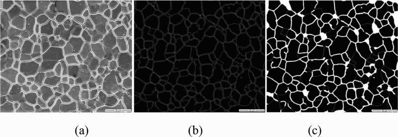
Grain segmentation: a sample micrograph; b output of Watershed algorithm; c final output after refinement

Determination of grain contours

Active contour models and its variants^21,22 are widely used to determine the closed contour of the objects present in an image. For this purpose, an initial guess of the object contour is required. The final contour is then evolved through minimisation of an energy function. The energy function is defined based on the image feature (e.g., intensity gradient). It has an external energy component that guides the contour towards the object boundary, and the internal energy component resists the deformation of the contour. The major drawback of the active contour model is that it requires an initial guess for the contour of each object, and it fails for the touching objects. In our context, the micrograph consists of multiple grains. It is prohibitive for the user to provide the initial guess for the contour of each grain. Moreover, one grain touches another. Hence, the active contour model does not satisfy our requirement.

Watershed transform based algorithms^23–26 are also commonly used in image segmentation, and they also provide a closed contour of the objects present in the image. The concept of watershed was introduced in 1970s. Since then, many improvements have been made on it. In this approach, a gray scale image is considered as a topographic relief where intensity value is thought of as the altitude in the relief. The intuitive idea is to classify the landscape regions as catchment basins and watershed lines. Catchment basins are low altitude regions in the landscape that holds water, and watershed lines (as if, mountains) are of high altitude acting as the barrier between the basins. In a gray scale image, a dark/low intensity area corresponds to basin, and watershed lines are light/high intensity area. A drop of water falling on a topographic relief flows along a path and finally reaches local minima. Intuitively, the watershed of a relief corresponds to the limits of the adjacent catchment basins of the drops of water. The algorithm identifies the basins and the watershed lines separating the basins. In the context of our problem, the grains correspond to the basin, whereas the grain boundaries are the watershed lines.

Watershed based segmentation algorithms can be classified into two major categories. One category focuses on detecting the basins, and the other focuses on finding the watershed lines. Flooding^23,24 belongs to the first category. Such schemes have a tendency of oversegmenting the regions. In a micrograph, the intensity values within and across the grains (basins) vary, and flooding is likely to split a grain into multiple regions. Moreover, a flooding based approach does not preserve the contrast. A topological watershed²⁶ is directed towards the generation of watershed lines. A graph based implementation is provided in the work of Couprie et al.,^26,27 and the mathematical foundation of the work has also been established.²⁸ A topological watershed algorithm works with the gradient image. Thereby, instead of absolute intensity value, it relies on the local contrast. It focuses on the detection of the contour separating the adjacent basins. The detection uses a parameter (t) that specifies the minimal altitude separating the catchment basins. Physically, t can be interpreted as the contrast between the grain interior and the grain boundary. Topological watershed preserves contrast and provides closed contour of the grains as desired in our study.

Applying the topological watershed algorithm, the closed contours of the regions are obtained. The value of the parameter t needs to be chosen carefully. A low value of t oversplits a region as it becomes sensitive to smaller intensity variation. On the other hand, a high value of t will accommodate more variation within a region and overlook weak boundaries. In our experiment, a moderate value for t is estimated, which approximates the contrast between the grain region pixels (low intensity value) and boundary pixels (high intensity value), and t has been taken as 2*σ, where σ is the standard deviation of the intensity values present in the image. The extracted contour for the grains shown in Fig. 3a has been presented in Fig. 3b, where the white lines are the contour lines.

Refinement of contour

The grain boundaries detected by the watershed algorithm are shown in white in Fig. 3b. However, all the enclosed regions shown in black are not grains. It is observed in Fig. 3a that the grain boundaries are quite thick because of the deep etching used to reveal them. As a result, the watershed algorithm detects the contrast difference around both inner and outer contours of the white thick boundaries. Finally, all the edges of the thick boundaries are extracted as watershed lines. The small patches enclosed between such lines are also identified as basins (grains). Thus, refinement is required to get rid of such regions that are actually part of the boundary. It is achieved by removing the black regions that are of very small area or by applying morphological closing operation.²⁹ It may be noted that in this process very small grains may be missed out. Figure 3c shows the final output of segmentation obtained after applying the refinement process on Fig. 3b. The black region enclosed within the white boundary corresponds to a grain.

Tracking of grains

Once the grains are segmented, each of them has to be uniquely marked in every sequential micrograph. Given the sequence of micrograph, correspondence between the grains also has to be established to enable the measurement of strain at grain level. It involves two steps:

Component labelling

Finding grain correspondence across the micrographs

In the segmented output, black pixels are part of the grain. Component labelling^29,30 starts with a black pixel and marks it with a label. It also marks the black pixels in its four-neighbourhood with the same label. The process goes on recursively with newly marked pixels. It stops when no further growth is possible. Thus, all the pixels in a particular grain are marked with the same label. The process then continues starting from another unmarked black pixel with a new label. Thus, when no unmarked black pixel is available, all the grains in the micrograph are uniquely labelled.

Pixels with same label belong to same grain. Because of the deformation, grains may undergo changes in terms of their size, shape, displacement and physical orientation. Thus, corresponding grains in two consecutive micrographs may not bear the same label. Therefore, it is not possible to link them based on the assigned labels. In this work, we establish the correspondence based on the proximity of the centroid (CG) of the grains in the consecutive micrographs in the sequence. 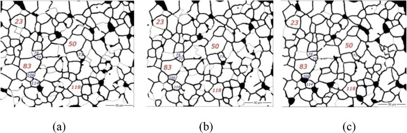The CG of a grain is computed based on the spatial moments.²⁷ The moment of order (p, q) of a grain can be defined by (1) where f (r, c) is the intensity of the grain pixel at (r, c), r and c spread over the grain. m(0,1) and m(1,0) are the first order moments. m(0,0) is known as the mass of the object. The coordinate of the CG is computed as follows (2) The CGs of the grains are computed in each micrograph. Let (r_ij, c_ij) denote the CG of a grain g_i in the ith micrograph. Corresponding to (r_ij, c_ij), the nearest CG is searched in the (i+1)th micrograph. Suppose the nearest one corresponds to the grain g_k in the (i+1)th micrograph. Then, g_i is tracked as g_k in the next micrograph. The process continues over the pairs of successive micrographs, and thereby, the grains are linked. Figure 4 shows the tracking of a few marked grains.

Tracked grains in sequence of micrographs: a reference micrograph, b and c corresponding micrographs under deformed condition

Strain measurement: DIC based technique

For measuring the grain level strain, the intensity values of each micrograph are first normalised. It reduces the impact of contrast/brightness variation (if any) during the capturing of different images. After tracking the individual grain of interest in the series of micrograph, a two-dimensional grid is drawn on that grain for correlation among consecutive images. In this technique, physical grids are not laid on the specimen surface as practised by lithography.^31–34 But in this experiment, an imaginary grid is placed on the reference image. It has been done in a manner so that the grid covers the grains over the area of interest on the specimen surface (Fig. 5a). The corresponding grid patterns on subsequent images of the deformed specimen are generated by the correlation technique, as shown in Fig. 5b–e.

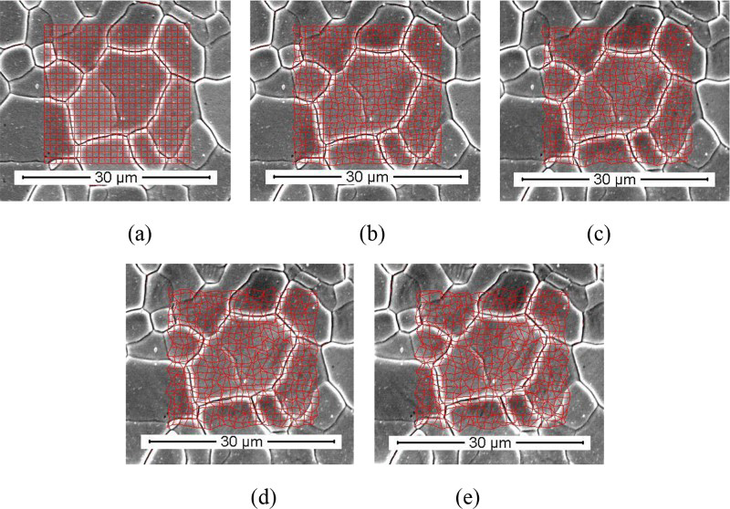
a grid drawn on portion of reference micrograph and b–e grid drawn by DIC technique on corresponding portion of subsequent micrographs

Correlation among the consecutive micrographs has been established using intensity based similarity. The schematic diagram of image correlation process is shown in Fig. 6. An imaginary grid is placed on the reference image. Figure 6a shows such horizontal and vertical grid lines in red colour, and the black squares represent the image pixels. Red squares formed by the intersecting grid lines are referred as subgrids. Each subgrid covers a small region of an image (10 × 10 pixels in our case). Let S_r denotes the set of intersection points of the vertical and horizontal grid lines (i.e. corner pixel of the subgrids) in the reference image. Corresponding to each element in S_r, the corresponding pixel in the next image is determined using intensity based correlation. Let p be an element in S_r with coordinates (X_p, Y_p). There may be a number of pixels in the next image with intensity similar to that of p. To surmount this problem, block matching is considered instead of individual pixel intensity based matching. This is similar to the commonly used approach in estimating the motion in video.

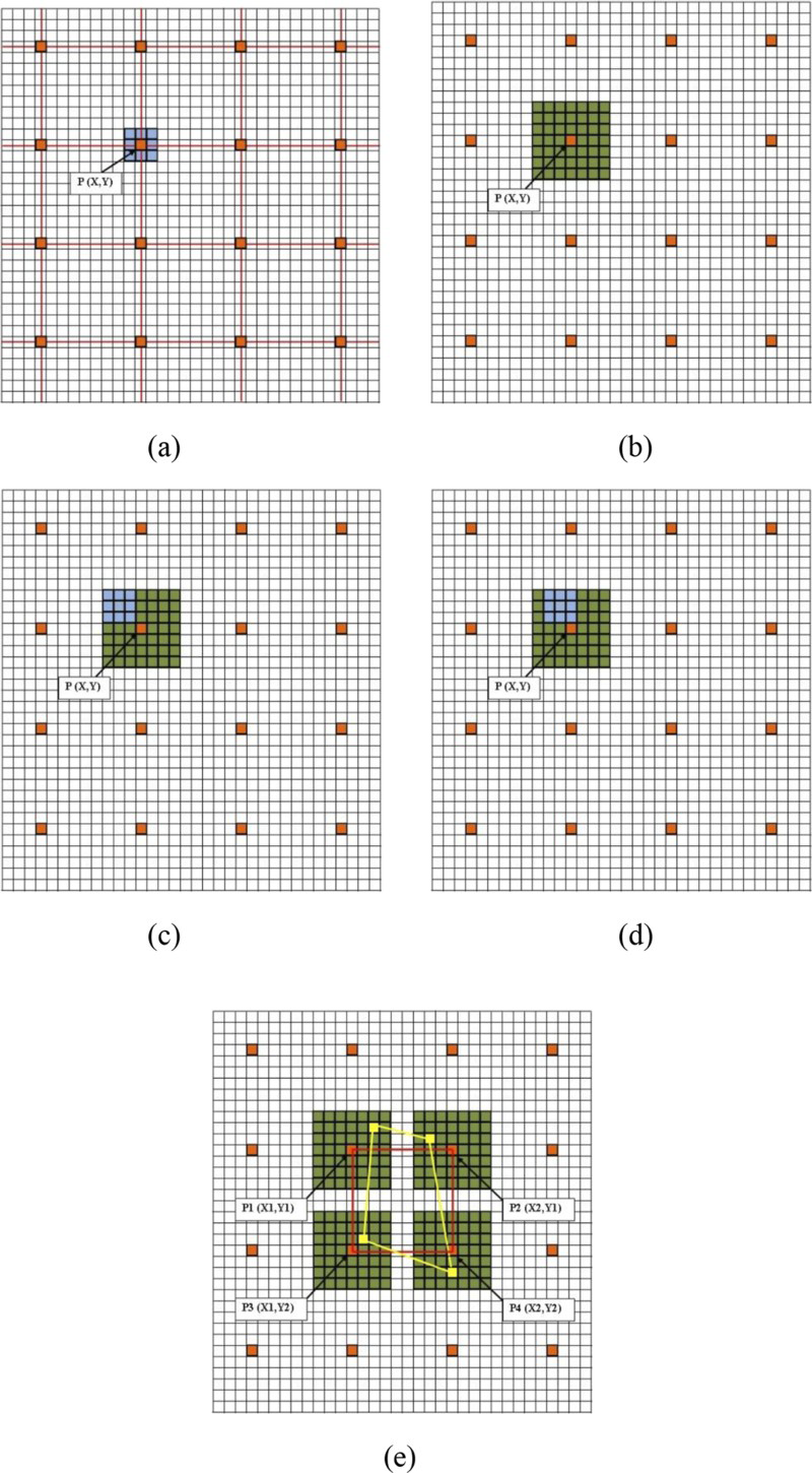
a imaginary grid and block of 8-neighbour pixels (in blue) corresponding to P(X, Y), subgrid corner in reference image; b search window (in green) for P(X,Y) in image following reference image; c, d search process to find match for block around P(X,Y) in search window; e subgrid of reference window (in red) and corresponding deformed subgrid (in yellow) superimposed on reference image

As shown in Fig. 6a, a block Br (in blue) centred at p is taken. In our case, the size of the block is 3 × 3 pixels, and it comprises of the pixel p along with its 8-neighbours. To search the best match for B_r, a search window (SW) is considered in the next image. The search window is of size K × K (must be larger than the block size), and it is centred at (X_p, Y_p), as shown in green in Fig. 6b. In our experiment, K is taken as 11. The best match for B_r is exhaustively searched in SW. A few cases are shown in Fig. 6c and d . B_r and a block in SW are compared based on the sum of absolute difference (SAD) of the intensity values of corresponding pixels in the blocks. The block in SW with minimum SAD is the adjudged as the match for B_r. The centre pixel of the matched block in SW is taken as the correlated pixel for p. Thus, for each pixel in S_r, a set of correlated points (S_c) in the next image is obtained. Figure 6e shows four corner points of a subgrid of reference image in red, and correlated points are in yellow. Correlated points corresponding to each side of the reference subgrid are joined by straight lines, and a deformed subgrid (shown in yellow) is obtained. To continue the correlation process for the subsequent images, S_c obtained in the previous step is taken as S_r for the next image, and the same process is followed.

To measure the grain level strain at a load, we restrict ourselves within the part of the grid covering the grain of interest. Let the rectangular bounding box with upper left corner (X_l, Y_l) and bottom right corner (X_r, Y_r) enclose the grain in the reference micrograph. After deformation, the bounding box may vary. To accommodate such variation, the rectangular region of the grid with upper left corner (X_l − 20, Y_l − 20) and bottom right corner (X_r +20, Y_r +20) in the reference micrograph is considered. Furthermore, the subgrids lying in the grain interior are taken into consideration for strain measurement.

Let the length of a side of the subgrids in the reference micrograph be l₀, and l be the length of the corresponding side on the micrograph of subsequent image in the loading direction. Then, the strain is calculated as [(l − l₀) / l₀]. The average strain of the grain is determined by averaging the strain of all such sides that are inside the grain. It should be noted here that the deformation of all the subgrids does not always follow the same direction as that of the applied load. As a result, in presence of tensile load, negative deformation of the subgrids frequently occurs. However, the overall deformation of individual grain consisting of subgrids has been found positive. Few grains over which the experiment has been carried out are marked in the reference image and shown in Fig. 7. The average strains for these grains on varying stress are shown in Fig. 8. The detailed strain distribution over the marked grains is also studied. Figure 9 shows the strain distribution over the grain marked 50, as an example, for different load values. The figure also shows the global strain of the particular grain at different loads. Note that the x axis represents the subgrids in the grain in raster scan order.

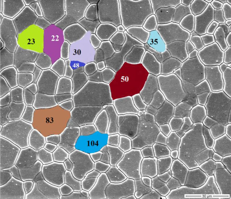
Marked grains in reference image

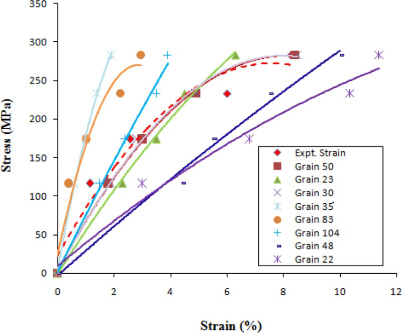
Stress–strain behaviour of different grains obtained using DIC method; macroscopic behaviour is shown in dashed line

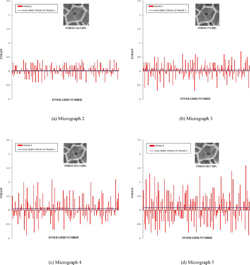
Strain distribution of individual subgrid over grain 50

Discussion

It is known that plastic deformation of metals and alloys occurs through movement of dislocations on slip planes. This mechanism of plastic deformation is known as slip. Although each grain of a polycrystalline material is in itself a single crystal, the orientation difference of the grains with respect to the loading axis does not permit all the grains to deform to the same extent. In the present study, it is observed that the slip lines (identified by red circle in Fig. 2c) become visible only when stress exceeds 174 MPa. The corresponding global strain at this load level is 2.56 pct. The slip lines are oriented at 45° to the loading axis, which coincides with the horizontal direction of the micrographs. It should be noted that using standard tensile specimen, the experimentally determined tensile yield strength of the steel is found as 189 MPa. The difference of 15MPa between the measured yield strength and the stress corresponding to the first visible slip lines in some grains arises from the differences in tensile deformation behaviour between macroscale and microscale (grain scale). With further increase of load, the slip lines become prominent and found in many grains as expected. All these observations point to the fact that all the grains do not deform to the same extent and at the same instant. The reason behind such grain to grain variation in strain arises because of the orientation difference of the grains with respect to the loading axis.³⁵

To verify the above conclusion, a methodology has been developed based on the DIC technique to estimate the local strain. It is found that all the grains do not deform to the same extent, but the extent of average deformation of any grain increases with the increase of load. Similar heterogeneous deformation in tensile deformed 1 mm thick commercial interstitial free steel has also been reported by Ghadbeigi et al.³⁶ In order to find the grain level strain, we have selected the grains quite arbitrarily and run our programme. It is observed that all the selected grains do not deform plastically within the experimental domain, and these grains are termed as hard grains; hard in the sense of their orientation with respect to the loading axis. In the present investigation, it is observed that one or two grains out of eight different grains studied follow the global deformation pattern. Ghadbeigi et al.³⁶ also reported a similar observation in interstitial free steel, even for very large global deformation.

The methodology that has been developed and followed for measuring grain level strain also brings out that even within a grain there is substantial point to point variation of deformation. This variation also exists in those grains that closely follow the global specimen deformation. The point to point variation of strain within a grain leads to infer that the very local activation of slip systems even within a grain is different. However, detail characterisation of the activation of slip systems in individual grains using electron back scatter diffraction technique is necessary to support this inference. Qualitatively, it is also found that the density of slip lines is less in those grains that are comparatively smaller in size. This observation is well connected with the well known Hall–Petch relationship. According to the Hall–Petch relationship, plastic deformation becomes difficult with lowering of grain size. It means that with lowering of grain size, the onset of plastic deformation occurs at higher load. It should be noted that the present methodology to find the grain level strain fails at large global deformation. This happens because of the undulation of the specimen surface due to out of the plane movement of the grains.

The DIC methodology developed and used in the present study for measuring local strain is, however, not free from error. The sources for error are (i) the difficulties associated with correlating the subgrid corners in deformed images and (ii) drifting of electron beam in SEM. The difficulty of correlating the subgrid corners also arises with change of contrast and brightness of the images of deformed specimens. To minimise the corresponding error, normalisation of intensity values in all images has been done at the very beginning. Besides, to correlate the subgrid corners instead of point matching, a block based matching has been adopted. The best match for the block of size 3 × 3 centred at the subgrid corners (say, coordinate x,y) has been searched in a bigger search window of size 11 × 11 centred at (x,y) in the next image. The concept of block has been used so that it captures the neighbourhood of the particular point. Such procedure minimises the possibility of mistracking of the subgrid corners. Tracking of the grains over the series of micrographs and matching the blocks in a bigger search window minimise the error introduced by drifting of electron beam.

In our study, we have estimated the error over a number of reference images, that is, of undeformed specimen, captured at different time intervals, which is about 5 minutes. Hence, the effect due to drifting of electron beam remains in the captured images. Additionally, to find the effect of brightness/contrast on the correlation process, the images of specimens were captured at different brightness/contrast levels. Based on the proposed image correlation technique, it has been found that the error associated with the tracked grains lies within the range of 0.1 to 0.6. The error range takes account of all sources of error.

Implementation of our methodology on images of tensile deformed IFHS steel shows that for a global strain of 8.26 pct, the average strains of the marked grains (Fig. 7) are different. As an example, while for grain no. 35, the average strain is 1.9 pct, and it is 11.37 pct for grain no. 22. As already mentioned, such a large variation in the average strain at the grain level arises due to orientation difference of the grains with respect to the loading axis. In our study, we also found grain to grain variation in the maximum local strain value in the loading direction. In conformity with the observation of Ghadbeigi et al.,³⁶ in our study, it is also found that local maximum tensile strain varies across the grains. For example, while the local maximum tensile strain is 180 pct in grain no. 83, it is 70 pct in grain no. 48.

Conclusions

From the results and discussion presented above, it is concluded that tensile deformation of the investigated IFHS steel occurs heterogeneously. The heterogeneity of deformation not only exists among different grains but also within a grain itself. The DIC methodology developed to segment and track the grains considerably reduced the error in measuring the grain level average strain and also the local strain within a grain varying between 0.1 and 0.6 pct. This error value also takes into account the error due to contrast/brightness of the images. The present methodology is capable to segment and track all the grains without any intervention of the user. Finally, the technique developed measures the average strain and local strain of each grain. However, it is necessary to incorporate electron back scattering diffraction characterisation of the specimen in the undeformed and deformed conditions at the individual grain level so to correlate the slip system activation of the individual grain with the measured strain. The beauty of the present methodology is that it uses artificial grids over the images and does not require any other sophisticated experimental technique to lay the grids on the specimen surface itself. The present methodology reveals that deformation is heterogeneous, and for an applied global strain of 8.26 pct locally within the grain interior, strain is magnified by many times reaching as high as 150 percent. Further, this local magnification of strain increases with the increase of global strain.

Footnotes

Acknowledgement

The authors deeply acknowledge the Ministry of Steel (GOI) and TATA Steel Ltd., Jamshedpur, India, for providing research grant (file no. 11(7)/SDF/2007-TW) to create the experimental facility and carry out the investigation.

References

Hashimoto

and Margolin

: ‘The role of elastic interaction stresses on the onset of slip in polycrystalline alpha brass-I Experimental determination of operating slip systems and qualitative analysis’, Acta Metall., 1983, 31, 773–785. doi: 10.1016/0001-6160(83)90093-7

Musienko

, Tatschl

, Schmidegg

, Kolednik

, Pippan

and Cailletaud

: ‘Three-dimensional finite element simulation of a polycrystalline copper specimen’, Acta Mater., 2007, 55, 4121–4136. doi: 10.1016/j.actamat.2007.01.053

Kamaya

, Kawamura

and Kitamura

: ‘Three-dimensional local stress analysis on grain boundaries in polycrystalline material’, Int. J. Solids Struct., 2007, 44, 3267–3277. doi: 10.1016/j.ijsolstr.2006.09.020

Raabe

, Sachtleber

, Zhao

, Roters

and Zaefferer

: ‘Micromechanical and macromechanical effects in grain scale polycrystal plasticity experimentation and simulation’, Acta Mater., 2001, 49, 3433–3441. doi: 10.1016/S1359-6454(01)00242-7

Makarov

P. V.

, Schmauder

, Cherepanov

O. I.

, Yu

, Smolin

V. A.

, Ramanova

R. R.

, Balokhonov

, Saraev

Yu.

, Soppa

, Kizler

, Fischer

, Hu

and Ludwig

: ‘Simulation of elastic-plastic deformation and fracture of materials at micro-, meso- and macro levels’, Theor. Appl. Fract. Mech., 2001, 37, 183–244. doi: 10.1016/S0167-8442(01)00078-7

Rusinko

: ‘Non-classical problems of irreversible deformation in terms of the synthetic theory, Acta Polytech’, Hung, 2010, 7, (3), 25–62.

Gunel

E. M.

and Basaran

: ‘Micro-deformation mechanisms in thermoformed alumina trihydrate reinforced poly (methyl methacrylate)’, Mater. Sci. Eng. A, 2009, A523, 160–172. doi: 10.1016/j.msea.2009.05.064

Kurzydlowski

K. J.

: ‘Microstructural refinement and properties of metals processed by severe plastic deformation’, Bull. Pol. Acad. Tech. Sci., 2004, 52, (4)

Okipnyi

, Maruschak

, Sorochak

and Sergejev

: ‘Measurement of deformation hardening of heat-resistant steel of the WWER-type reactor’, Proc. 8th Int. DAAAM Baltic Conf. on ‘Industrial engineering, Tallinn, Estonia, April 2012, DAAAM Baltic, Tallinn University of Technology, 694–699.

10.

Piwnik

and Mogielnicki

: ‘Deformations in micro extrusion of metals’, Arch. Foundry Eng., 2010, 10, (3), 87–90.

11.

Pradhan

P. K.

, Dash

P. R.

, Robi

P. S.

and Roy

S. K.

: ‘Micro void coalescence of ductile fracture in mild steel during tensile straining’, Frattura ed Integrità Strutturale, 2012, 19, 51–60.

12.

Qian

, Xie

and Asundil

: ‘Two dimensional digital image correlation for inplane displacement and strain measurement: a review’, Meas. Sci. Technol., 2009, 20, (6)

13.

Ulstad

M. S.

: ‘An algorithm for estimating small scale differences between two digital images’, Pattern Recognit., 1973, 5, (4), 323–333. doi: 10.1016/0031-3203(73)90024-1

14.

Sjodahl

: ‘Electronic speckle photography: Increased accuracy by non integral pixel shifting’, Appl. Opt., 1994, 33, (28), 6667–6673. doi: 10.1364/AO.33.006667

15.

Cintron

and Saouma

: ‘Strain measurements with the digital image correlation system Vic 2d’, ‘Technical report, University of Colorado, Boulder, CO, USA’; 2008.

16.

Rugg

: ‘Materials for future gas turbine applications’, Mater. Sci. Technol., 2014, 30, (15), 1848–1852. doi: 10.1179/1743284714Y.0000000609

17.

Davenport

J. R.

, Mendez-Garcia

, Purkayastha

, Hancock

M. E.

, Stearn

R. J.

and Clegg

W. J.

: ‘Material needs for turbine sealing at high temperature’, Mater. Sci. Technol., 2014, 30, (15), 1877–1883. doi: 10.1179/1743284714Y.0000000527

18.

Kang

: ‘Microscopic strain mapping based on digital image correlation’, Int. Cong. Expo. on Experimental and Applied Mechanics, Society for Experimental Mechanics, Orlando, FL, USA; 2008.

19.

Gom

: ‘Aramis-deformation measurement using the grating method’, User's Manual, V5.3.0-8, Braunschweig, Germany; 2003.

20.

Cao

, Bi

, Wei

and Xie

: ‘Determination of poissons ratio of kraft paper using digital image correlation’, Mech. Eng. Technol. Adv. Intell. Soft Comput., 2012, 125, 51–57. doi: 10.1007/978-3-642-27329-2_8

21.

Kass

, Witkin

and Terzopoulous

: ‘Snakes: active contour models’, Int. J. Comput. Vision, 1988, 1, (4), 321–331. doi: 10.1007/BF00133570

22.

McInerney

and Terzopoulous

: ‘T-snake: Topology adaptive snakes’, Med. Image Anal., 2000, 4, (2), 73–91. doi: 10.1016/S1361-8415(00)00008-6

23.

Beucher

and Lantuéj

: ‘Use of watershed in contour detection’, Int. Workshop on ‘Image processing, real-time edge and motion detection’, Rennes, France, 1979. Available at: http://cmm.ensmp.fr/beucher/publi/watershed.pdf.

24.

Meyer

and Beucher

: ‘Morphological segmentation’, J. Visual Commun. Image Represent., 1990, 1, (1), 21–46. doi: 10.1016/1047-3203(90)90014-M

25.

Beucher

: ‘The watershed transformation applied to image segmentation’, Scanning Microsc., 1992, 299–314.

26.

Couprie

and Bertrand

: ‘Topological grayscale watershed transform’, SPIE Vision Geom. Proc., 1997, 3168, 136–146. doi: 10.1117/12.292778

27.

Couprie

, Najman

and Bertrand

: ‘Algorithms for the topological watershed’, Proc. Int. Conf. on ‘Discrete geometry for computer imagery, Poitiers, France, April 2005; Springer, 172–182.

28.

Bertrand

: ‘On topological watersheds’, J. Math. Imaging Vision, 2005, 22, (2-3), 217–230. doi: 10.1007/s10851-005-4891-5

29.

Chanda

and Majumder

D. D.

: ‘Digital image processing and analysis’; 2009, New York, Prentice Hall India.

30.

Gonzalez

R. C.

and Woods

R. E.

: ‘Digital image processing’; 1992, Upper Saddle, NJ, Prentice Hall.

31.

Stoshi

, Kazuhiro

, Yanada

, Minami

, Kimura

and Ikeda

: ‘Direct drawing method for microfabrication based on selective metal plating technology’, Sens. Actuators A, 103A, 2003, 135, 142.

32.

Jacobsen

S. C.

, Wells

D. L.

, Davis

C. C.

and Wood

J. E.

: ‘Fabrication of micro-structures using non-planar lithography (NPL)’, Proc. MEMS’91, Nara, Japan, January 1991, IEEE. 74–79.

33.

Beuret

, Racine

G. A.

, Gobet

, Luthier

and Rooij

N. F.

: ‘Microfabrication of multidirectional inclined structure by uv lithography and electroplating’, Proc. MEMS'94, Oiso, Japan, January 1994, IEEE, 81–85.

34.

Konishi

, Honsho

and Sugiyama

: ‘Direct drawing for micro-fabrication without photolithography’, Proc. MEMS'99, Florida, USA, January 1999, IEEE, 194–199.

35.

Tschopp

M. A.

, Bartha

B. B.

, Porter

W. J.

, Murry

P. T.

and Fairchild

S. B.

: ‘Microstructure dependent local strain behaviour in polycrystals through in-situ scanning electron microscope tensile experiments’, Metall. Mater. Trans. A, 2009, 40A, (10), 2363–2368. doi: 10.1007/s11661-009-9938-6

36.

Ghadbeigi

, Pinna

and Celotto

: ‘Quantitative strain analysis of the large deformation at the scale of microstructure: comparison between digital image correlation and microgrid techniques’, Exp. Mech., 2012, 52, (9), 1483–1492. doi: 10.1007/s11340-012-9612-6