An overview of first-principles calculations of NMR parameters for paramagnetic materials

Abstract

Many technologically important materials exhibit paramagnetism, for example, lithium intercalation materials for lithium-ion batteries and platinum nanoparticles for catalysis. In order to study their properties, for example, their electron transport properties or catalytic efficiency, and hence tailor them to specific engineering applications, information on their structure and bonding needs to be acquired. Solid state nuclear magnetic resonance (NMR) is an excellent experimental method for achieving this; however, the resulting spectra are often difficult to interpret. Calculations based on quantum mechanics therefore provide an invaluable aid for decoding these experimental spectra.

The dominant interaction in paramagnetic materials is the hyperfine interaction. This is the interaction between the spin of a nucleus and the spin of an unpaired electron. The hyperfine interaction affects the appearance of NMR spectra, both by shifting the frequencies at which resonance occurs and by removing degeneracies so that a single resonance frequency splits into several frequencies. This review examines the methods and current limitations for calculating hyperfine interaction parameters, placing this in the context of experimental NMR investigations for lithium intercalation materials and platinum nanoparticles. In this way, the importance of developing increasingly accurate methods for calculating hyperfine parameters is illustrated.

Literature review motivation

Nuclear magnetic resonance (NMR) is an extremely powerful and flexible experimental technique. It employs the sensitivity of a nuclear spin to its atomic environment to probe the structure and bonding of the material and hence provide insight into the material's mechanical, electrical, magnetic and chemical properties. Owing to its high sensitivity and transferability, NMR now forms part of the standard tool kit at the experimentalist's disposal.

The large number of interactions influencing the behaviour of the nuclear spins results in experimental spectra being difficult to analyse. While it is often possible to interpret experimental NMR spectra for liquids, solid-state spectra present a greater challenge. This is because the inherent anisotropy of solids leads to a high degree of broadening of the peaks about the resonant frequencies, which makes the individual contributions of different interactions harder to separate. Simulated NMR spectra are therefore an invaluable tool for decoding the experimental spectra. They can also be used to predict the properties of exotic materials in advance of conducting experiments and therefore guide the experiments themselves.

The simulations for solid-state NMR are obtained using a first-principles approach, without the use of empirical parameters. Since the resonance of nuclear spins is a fundamentally quantum mechanical phenomenon, the calculations are based on solving the quantum mechanics of the system. Such calculations would not have been possible in practice were it not for theoretical advances such as density functional theory (DFT), the development of iterative algorithms as implemented in modern codes and high performance computers.

It is currently possible to calculate relevant NMR parameters for diamagnetic materials.^1–3 These calculations have proved so successful that the methodology has been widely adopted by the experimental community.^4,5 The methodology for first-principles calculations of NMR parameters for paramagnetic materials (those materials containing unpaired electrons) has yet to be fully developed.

The dominant interaction in the NMR of paramagnetic materials is the hyperfine interaction. This is the interaction between the spin of a nucleus and the spin of an unpaired electron. Of particular importance is the isotropic component of the hyperfine interaction, the Fermi contact term, which manifests in a wide range of materials science applications, including lithium-ion cathode materials and platinum nanoparticles for catalysis.

Introduction to magnetic resonance

In 1922, Stern and Gerlach discovered that nuclei possess their own intrinsic magnetic moment (spin).⁶ Just over a decade later, Stern, continuing his molecular beam experiments along with Estermann and Frisch, succeeded in measuring the magnetic moment of the proton.^7–10

Rabi is often credited with inventing the magnetic resonance technique. In 1938, building on Stern and other's achievements and the under-acknowledged work of Gorter,¹¹ he and his group succeeded in measuring the frequency at which the magnetic moment of lithium atoms resonated in a beam of LiCl molecules (see Fig. 1.¹² A year later, they measured the magnetic resonances of Li⁶, Li⁷ and F¹⁹ in LiCl, LiF, Li₂ and NaF molecules.¹³ His achievements earned him the 1944 Nobel Prize in Physics.¹⁴

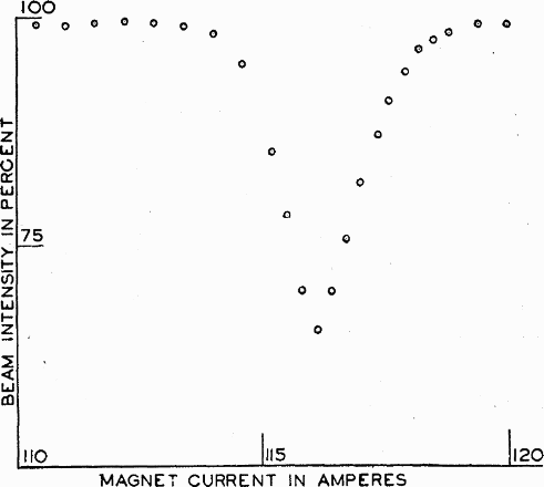
The first magnetic resonance spectrum from Rabi et al.¹² (reproduced in Hurwitz¹⁶). This was obtained by Rabi et al. for lithium in a molecular beam of LiCl. ‘MAGNET CURRENT IN AMPERES’ relates to the magnitude of the homogeneous magnetic field. Rabi and his group found that this produced more accurate results than the modern method of keeping the magnetic field constant and varying the frequency of the radiation. ‘BEAM INTENSITY IN PERCENT’ refers to the intensity of the LiCl beam. The plot minimum occurs at the resonance frequency of the lithium atoms (reprinted from Ref. 12 with permission: © 1938 American Physical Society)

Since then, the supreme sensitivity and transferability of the technique has resulted in countless applications in chemistry, physics, biology, materials science and medical imaging, and has produced an additional six Nobel Prizes. An excellent review on the early history of magnetic resonance has been written by Ramsey.¹⁵

Principle of magnetic resonance

Nuclei possess an intrinsic spin angular momentum, I, and with it an associated spin magnetic dipole moment μ_I according to 1 γ is the gyromagnetic ratio for a nucleus, which can also be expressed as , where g_I is the dimensionless g-factor for a free nucleus, μ_N is the nuclear magneton and ħ is the reduced Planck constant. The magnitude of γ is specific to each isotope and is expressed in terms of 10⁷ rad T^− 1 s^− 1, or sometimes MHz^− 1 T^− 1, with a conversion factor of 2π between the two units.

When there is no external magnetic field, all nuclear spin I orientations are degenerate. Applying an external magnetic field, B ₀, however, removes the degeneracy in the spin states, such that the energy, E, of a certain spin state is given by

2 where B is the magnetic field experienced by a certain nucleus. The energy difference, ΔE, between two spin states increases according to 3 where m is the magnetic quantum number. An external pulse of electromagnetic radiation of frequency, ν, may excite a spin state into a higher energy spin state provided that the resonance condition, (where h is Planck's constant) and the transition selection rule, Δm = ± 1, are satisfied. Thus, the frequency of the radiation required for NMR, termed the Larmor frequency, is 4 Equations (2)–(4)) contain the local magnetic field experienced by the nucleus, B. This differs from the external magnetic field, B₀, because B₀ induces current loops in the surrounding electrons, which in turn induce an additional local magnetic field that is also experienced by the nuclear magnetic moment. This leads to a chemical shift, δ, in the resonance frequencies, which is specific to the chemical environment, thus enabling valuable information to be deduced about the structure and bonding of a sample.

The additional local magnetic field, B_in, is related to the applied magnetic field, B₀, through the absolute magnetic shielding tensor, σ, by 5 Under isotropic conditions, such as in solution-based NMR or solid-state NMR under magic angle spinning (MAS) (see the ‘Solid-state NMR’ section), the anisotropic components average out so that σ becomes the isotropic shielding σ_iso (a third of the trace of σ).

Experimentally, the chemical shift, δ, is measured relative to a standard reference σ_ref so that δ is conventionally defined as 6 A good introduction on NMR is, for example, presented in Hore's book.¹⁷

Hyperfine interaction

In the field of magnetic resonance, the hyperfine interaction is defined as the interaction between the spin of the nucleus, I, and the spin of the electron, S (Refs. 18, p. 211 and 19, p. 97).

The Hamiltonian for hyperfine coupling, , can be expressed as the interaction between the magnetic dipole moment, μ_I, of the nucleus with the magnetic field generated by the atomic electrons, B_e, according to 7

Since the nuclear spin magnetic dipole moment, μ_I, is directly proportional to I (equation (1)), and B_e is directly proportional to the total angular momentum of the electron J (Ref. 19, p. 97–101), equation (7) becomes 8 where A is a constant. For light elements, relativistic effects do not have a measurable effect on the hyperfine interaction.^20,21 In these cases, spin orbit effects can be excluded and the hyperfine Hamiltonian can be expressed as 9

Incorporating into the hyperfine Hamiltonian the interaction between the electron and M nuclear spins I_l, where l denotes the l^th nucleus at position R _l, equation (9) becomes 10 where A^(l) is the hyperfine coupling tensor for the l^th nucleus.²² This can be separated into two parts corresponding to the isotropic Fermi contact interaction and the anisotropic spin–dipolar interaction according to 11 where a^(l) is the isotropic hyperfine (Fermi contact) interaction, is the anisotropic hyperfine (spin-dipolar) interaction, δ_ij is the Kronecker delta, and i and j are cartesian axes.

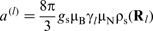
Physically the Fermi contact interaction is the magnetic (spin–spin) interaction between the electron and the nucleus when the electron is inside the nucleus. The strength of the Fermi contact interaction is directly proportional to (Ref. 23, p. 465) and can therefore be expressed in atomic units as 12 where ρ_s(R_l) is the electron spin density ( ) at the centre of the l^th nucleus, γ_l is the gyromagnetic ratio for the l^th nucleus, g_s is the dimensionless g-factor for a free electron, γ_e is the gyromagnetic ratio for a free electron, μ_B is the Bohr magneton and μ_N is the nuclear magneton.²² Since ρ_s is directly proportional to the square of the electron wavefunction at the centre of the nucleus, , the Fermi contact interaction is only affected by s-like electrons, because only s-like wavefunctions are non-zero at the nucleus. The calculation of poses several computational problems outlined in the ‘First-principles calculations of hyperfine parameters’ section. By contrast, the spin–dipolar interaction is affected by non s-like electrons.

The hyperfine interaction emerges as a large measurable shift in resonance frequencies in paramagnetic NMR spectra. It is related to the Knight shift in the NMR of metallic systems (see the next section).

Knight shift

First observed by Knight in 1949,²⁴ this is a systematic shift in the resonance frequencies of metallic systems, which is not observed in the resonance frequencies of the same element in non-metallic systems. To a first approximation, this shift occurs because an external magnetic field will induce a magnetisation, M, in the paramagnetic material. The magnetisation arises from the unequal change in energy of the conduction electrons (those close to the Fermi energy, E_F) between those with spin- and those with spin- . Thus, the material acquires a magnetisation, characterised by the average spin of the conduction electrons ⟨S_z⟩ or by the Pauli spin susceptibility χ_s, where (where g_s is the free electron g-factor and N is Avogadro's number). This net electron spin creates a magnetic field, additional to B ₀, which interacts with the nuclear spin magnetic moment via the hyperfine interaction. This produces a shift in energy levels, which manifests as a shift in resonance frequencies. The Knight shift, K, is defined as (Ref. 25, p. 478) 13 where a^(l) is the Fermi contact constant as defined for the l^th nucleus in equation (12). Thus, K is proportional to the value of the electron spin density at the nucleus according to 14 The theoretical evaluation of poses some difficulties as outlined in the ‘First-principles calculations of hyperfine parameters’ section.

The magnitude of the Knight shift at each crystallographically distinct nucleus in a sample will differ. This is observed as an inhomogeneous broadening in the resonance peak.²⁶

Solid-state NMR

The main difficulty when acquiring experimental solid-state NMR spectra is that there are very large amounts of line broadening due to the inherent anisotropy of the solid samples. This leads to difficulties pertaining to the sensitivity and resolution of spectra. Notable anisotropic interactions include shielding/chemical shift anisotropy (CSA), dipolar coupling (the interaction between two magnetic moments through space (Ref. 18, p. 24)) and quadrupolar coupling (an electric interaction affecting nuclei with spin greater than (Ref. 18, p. 28)). While it may be desirable to remove these interactions from spectra to aid interpretation, the interactions themselves can provide further valuable information about the sample. Dipolar coupling provides information on the distances between nuclei and atomic structure, CSA can provide structural information and J-coupling can provide information on chemical bonding and geometry. There therefore exist methods for selectively reintroducing interactions in spectra. An overview of the methods to both remove and reintroduce interactions is presented in Bonhomme et al.'s extensive review paper.⁴

The most common technique for removing broadening from CSA and dipolar coupling is MAS. Relevant interactions in NMR involve a dependency on the orientation of the crystal relative to the applied magnetic field of the form θ − 1, where θ is the angle between the crystallographic principal axis and the applied magnetic field. Associated broadening can therefore be removed by rapidly spinning the sample at the ‘magic angle’ 54.736° to the applied magnetic field. A detailed explanation can be found in Harris et al.'s book on solid-state NMR (Ref. 18, p. 32). Rotation rates tend to be 5–70 kHz⁴; however, rates of up to 110 kHz may be used.²⁷ In the case of paramagnetic materials, where there are unpaired electrons present, the anisotropy associated with the hyperfine interaction can be very large and therefore very high rotation rates are required in order to achieve spectra of a suitable resolution (Ref. 18, p. 213).

Despite the plethora of different techniques available for probing the structure, interactions and chemical environments in solids, the experiments are time consuming and restricted to certain systems, and it can be difficult to acquire spectra of sufficient resolution for analysis. Theoretical calculations of relevant NMR parameters therefore provide a much needed, if not essential, aid for the prediction and interpretation of experimental spectra in addition to valuable insights into the active mechanisms in a system.

Introduction to first-principles calculations

First-principles approaches aim to calculate properties of materials using only the postulates of quantum mechanics.²⁸ Since the mechanisms involved in NMR are quantum mechanical in origin, calculating their relevant parameters through this approach is most appropriate.

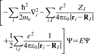
For a system containing electrons and nuclei, the time independent nonrelativistic Schrödinger equation, , can be expressed as 15 where r_i and R_I are the spatial coordinates of the electrons and nuclei respectively, M_I is the mass of the nucleus, m_e is the mass of the electron, Z_I is the absolute charge of the nucleus, ε₀ is the permittivity of free space and e is the charge of the electron (Ref. 28, p. 52). However, this cannot be solved exactly for more than a handful of electrons because the numerical calculation of the interaction between the electrons is too computationally expensive.²⁸ It therefore needs to be simplified.

Density functional theory

One method for simplifying equation (15) is the Hartree–Fock method. This involves treating the interaction between electrons as an interaction between a single electron and the mean field of all the other electrons.²⁹ However, this is still computationally expensive for solid systems. DFT is a significantly cheaper alternative and has been widely adopted by theoretical and experimental communities for calculating NMR parameters.⁴

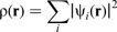
The DFT formalism begins from the premise that the total ground state energy, E₀, of a system is a unique functional of the total electron density, ρ, of the system, as formally proved by Hohenberg and Kohn in 1964³⁰: 16 Unfortunately, the functional E₀[ρ] cannot be exactly known. In 1965, Kohn and Sham found a way to get around this by assuming that there existed a system of fictitious non-interacting single electrons whose density was identical to that of the original ground state density of the interacting system.³¹ The many-body interactions were placed in an unknown exchange–correlation functional E_xc[ρ].

Thus, equation (15) becomes a set of single electron equations, which are coupled together through the electron charge density ρ(r) via

17 where is the single electron wavefunction.

The total energy E of the system can therefore be expressed as 18 where E_kin is the kinetic energy of the non-interacting electrons, E_N is the potential energy between the non-interacting electrons and the nuclei, E_H[ρ] is the Hartree energy which is the potential energy between each non-interacting electron and the mean field of the other electrons, and E_xc[ρ] is the exchange correlation energy.

These equations can be solved iteratively (see Fig. 2). However, to begin with, E_xc[ρ] still has to be approximated.

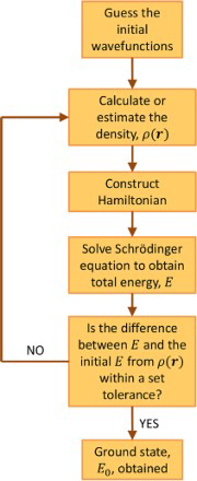
The iterative solving of the Kohn–Sham equations for the total energy, E. Self-consistency is reached when the difference in E between a set number of successive iterations is within a set tolerance

Exchange–correlation functionals

The simplest approximation for E_xc[ρ] is the local density approximation (LDA). This assumes that E_xc[ρ] depends only on the charge density at each point.^32,33 By additionally taking into account the gradient at each point, more advanced generalised gradient approximation (GGA) exchange–correlation functionals are obtained. The most commonly used exchange–correlation functional used for calculating NMR parameters is the GGA functional formulated by Perdew, Burke and Ernzerhof (PBE).³⁴

Practical implementation of DFT

In order to solve equation (18) in practice, a set of numerical approximations need to be made.

Basis set

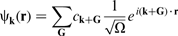
The wavefunction needs to be expressed as a ‘linear combination of simple mathematical functions’.⁴ These could be set of localised atom-centred orbitals, for example, the Gaussian type orbitals used in the CRYSTAL³⁵ and SIESTA³⁶ codes. Another possibility is a set of planewaves as used in the CASTEP code³⁷: 19 where k is an electron wavevector, G is a reciprocal lattice vector and Ω is the volume of the primitive cell. An energy cutoff is set to determine the maximum energy of the highest component plane wave.

Periodicity of structures

In order to reduce the number of atoms in the solid-state system to a computationally realistic level, the periodicity of the crystal lattice is exploited using Bloch's theorem (Ref. 25, p. 163): 20 where L is the real space lattice vector. Consequently, only the atoms within the first Brillouin zone need to be considered.

k point sampling

Calculating the charge density at a set of discrete points in the Brillouin zone provides a sufficiently accurate sum of the total charge density if enough points are sampled,

21 where N_k is the total number of points. These k points are chosen to form a grid as developed by Monkhorst and Pack.³⁸ Metallic systems, such as those exhibiting a Knight shift, require further care when setting these k points due to the partial occupancy of bands near the Fermi surface. In these cases, the contributions to the charge density at each k point may be smeared.^39–41

Pseudopotentials

Valence wavefunctions oscillate rapidly near the nucleus and therefore require a high energy cutoff in order to be accurately described. To reduce the energy cutoff, and thus increase computational efficiency, the potential close to the nucleus, defined within a radius r_c, is smoothed. This results in a pseudopotential and a correspondingly smoothed pseudowavefunction. Crucially, the energy eigenvalues are not affected. This is the pseudopotential approximation.

In most cases, only the valence electrons require pseudopotentials. The eigenvalues for the core electrons, since they are not involved in bonding, are assumed to be the same as those in an isolated atom and can therefore be easily calculated. This is the frozen core approximation. In the case of hyperfine parameters, this is not a valid approximation.

First-principles calculations of hyperfine parameters

The initial theory for calculating NMR parameters was developed by Ramsey in the 1950s.^42–44 Since then, computational methods pertaining to the NMR parameters for diamagnetic materials have been developed including the magnetic shielding tensor, σ, as defined in equation (5).^1,2 For metallic systems, there has been progress in the calculation of magnetic shielding tensors and Knight shifts.⁴¹ In terms of hyperfine parameters, early qualitative attempts to calculate Fermi contact shifts involved calculations on molecular solids using Hartree–Fock and DFT.^45–48 There is also wide interest in calculating the hyperfine interaction for single molecules (Refs. 29, 49, 50 and 51, p. 209).

Methodologies and challenges

In order to quantitatively calculate hyperfine parameters within the methodology outlined in the ‘Density functional theory’ section, two challenges must be overcome: (i)

Valence electrons—the wavefunctions for these are smoothed pseudowavefunctions within r_c. This leads to non-physical charge densities close to the nucleus and thus incorrect hyperfine parameters.

(ii)

Core electrons—these are calculated using the frozen core approximation. However, the spin of the valence electrons can cause spin polarisation of the core electrons. Because accurately computing the Fermi contact interaction relies on exactly knowing the spin density ( ) at the nucleus, failure to include this core polarisation will lead to significant errors.

Projector augmented wave method

Blöchl overcame the first challenge by recreating the true all-electron non-pseudised wavefunction for valence electrons from the pseudowavefunction within a region close to the nucleus bounded by a selected radius, r_c.⁵²

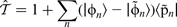
The pseudowavefunction is mapped onto the all-electron wavefunction by the operator according to 22 where 23 Within r_c, the pseudowavefunction is composed of a linear combination of pseudo atomic states . Equation (23) therefore corresponds to removing the section of located within r_c and replacing it with the equivalent all-electron atomic states . is a function strongly localised within r_c and is therefore used to ensure that only the section of within r_c is altered. A pictorial representation of equation (23) is given in Fig. 3.

Schematic of the projector augmented wave (PAW) method.⁵³ The x axis signifies the radial distance from the nucleus: a initial pseudowavefunction ; b two separate pseudo-atomic states ; c two corresponding all-electron atomic states ; d final reconstructed all-electron wavefunction (reprinted from Ref. 53 with permission: © 2010 Wiley)

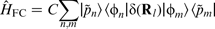
Extending the PAW methodology to the Fermi contact interaction results in the associated operator⁵³: 24 where C is a constant and δ(R_l) is the Dirac delta function positioned at the nucleus.

Core polarisation

Progress in overcoming the second challenge was begun by Yazyev et al. through the core spin–polarisation correction method.⁵⁴ Instead of calculating the core electron eigenstates from an isolated atom, the all-electron wavefunction for the core electrons was reconstructed in the presence of the valence electrons, with the valence states being approximated to those in an isolated atom. This produced a significant improvement on the Fermi contact term for a series of small molecules. Declerck et al. proposed an alternative hybrid method for the inclusion of core polarisation, which combined an all-electron calculation for the atom of interest with a pseudopotential calculation for all the others.⁵⁵ Not only could this hybrid method be applied to single atoms and small molecules, but it could also be applied to solids. The hyperfine interaction of the L-α-alanine R2 radical in a crystal of L-α-alanine molecules was calculated as an example of this. Bahramy et al. developed a further improvement through calculating the core polarisation using first-order perturbation theory.^56,57 In this way, the spin density at the nucleus was evaluated in two steps. First, the PAW method of Blöchl was used to reconstruct the all electron wavefunctions of the valence electrons within r_c. Second, the contribution to core polarisation from the core electrons was evaluated using first-order perturbation theory.⁵⁷ This methodology has been used by Filidou et al.²² to evaluate Fermi contact terms for small molecules and fullerene derivatives.

Materials applications

Lithium-ion battery materials and platinum nanoparticles are two paramagnetic systems that exhibit hyperfine interactions and are of significant importance to current and future engineering applications. The first-principles modelling methods discussed in the ‘Introduction to first-principles calculations’ and ‘First-principles calculations of hyperfine parameters’ sections provide an invaluable aid in the determination of their materials properties.

Lithium-ion battery materials

Lithium intercalation materials, as discussed here, are layered oxides with lithium ions in between the layers. Figure 4 shows the compound LiCoO₂ which formed the cathode in the first commercial Li-ion battery.⁵⁸ This has been widely used in laptops, mobile phones and cameras; however, the low abundance of cobalt makes it expensive to manufacture and it has a low theoretical charge capacity of ∼130 mAh g^− 1.⁵⁸ As a result, research on other lithium compounds is vast.⁵⁸

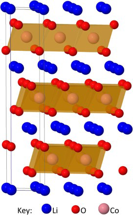
Structure of LiCoO₂, showing the layers of CoO₆ octahedra and Li⁺ ions

Solid-state NMR studies of cathode materials for lithium-ion batteries are extensive.^59,60 Spectra are dominated by interactions between electronic and nuclear spins, and exhibit Knight shifts (between the conduction electrons and nuclei) and other hyperfine shifts (between unpaired electrons and nuclei). Often, the ⁷Li and ⁶Li resonances are studied.^61–65 This is because neighbouring paramagnetic metal ions induce an electron spin density at the lithium nucleus, which experimentally emerges as large hyperfine shifts. Analysis of these hyperfine shifts provides insight into conduction mechanisms and structural changes from electrochemical recycling.

The hyperfine shift can be understood to originate from two competing mechanisms: spin delocalisation (or hybridisation) and spin polarisation.

Experimental hyperfine shifts

The Fermi contact shift has been experimentally measured in LiCoO₂,⁶⁶ and the related structure LiMnO₂.⁶⁷ These have an ABCABC layered ‘O3’ structure as characterised by Delmas et al. in their structural classification of the layered oxides.⁶⁸ Marichal et al. studied nickel doping of LiCoO₂.⁶¹ Other candidate compounds for which the hyperfine shifts have been measured include chromium doped LiCoO₂⁶⁶; the spinels LiMn_2 − xM_xO₄, for which LiMn₂O₄ has a large hyperfine shift >500 ppm in ⁶Li and ⁷Li MAS spectra^69–72; and lithium phosphates LiMPO₄, where M is Mn, Fe, Ni, Co,^73,74 La₄LiNiO₈,⁷⁵ La₄LiMnO₈,⁷⁶ and La₃SrLiMnO₈.⁷⁶

First-principles calculations

The first calculations of the hyperfine interaction in lithium-ion battery materials were conducted by Carlier et al.⁴⁸ They used DFT (see the ‘Density functional theory’ section) to calculate the electron spin density of the system and then integrated this within the vicinity of the nucleus to obtain the total electron spin density contributing to the Fermi contact shift. They used an integration radius of 0.8 Å, compared to the measured radius of a lithium ion in an octahedral site of 0.76 Å.⁷⁷ It is important to note that they used pseudopotentials with no PAW correction, which meant that their calculated charge density at the lithium nucleus was non-physical. This problem was partially bypassed because their integration radius would have been larger than the radius r_c within which the pseudopotential acted (see the ‘Pseudopotentials’ section), and so, they could assume that the integrated charge density was an indication of the hyperfine interaction. In most cases, their calculations display good comparisons to experiment. However, they also acknowledge that their calculations can only be used to predict the sign and rough magnitude of the shifts.

Interestingly, Carlier et al.'s calculations revealed that the previous assignment of experimental Ni peaks in the MAS NMR spectra for O₂ materials, by Marichal et al.,⁶¹ to Ni first and second nearest neighbours of the Li⁺ should have been reversed. Marichal et al. had used a set of generalised rules to assign the peaks. It had also been assumed that, out of the two competing mechanisms contributing to the hyperfine shift in these materials, the polarisation mechanism was negligible compared to the delocalisation mechanism. The calculations revealed that while delocalisation was important, there was also a significant contribution due to polarisation, leading to hyperfine shifts of opposite sign than previously supposed.

In the last decade, further calculations have been conducted using the CRYSTAL code.^78,79 Mali et al. used the PAW formalism to calculate the Fermi contact shift for ⁶Li in Li₂FeSiO₄ polymorphs⁸⁰ with excellent agreement to experiment (see Fig. 5).

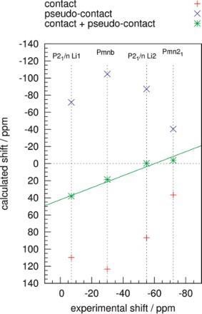
Comparison of calculated Fermi contact shifts (red cross) with experiment by Mali et al.⁸⁰ The pseudo-contact interaction is the spin–dipolar interaction expressed in equation (11) (reprinted from Ref. 80 with permission: © 2011 American Chemical Society)

Platinum nanoparticles

Platinum is a particularly interesting system to study using NMR. The only isotope that can be investigated using magnetic resonance is ¹⁹⁵Pt, which has a healthy abundance of 33.8 and a moderate gyromagnetic ratio of 5.80446 × 10⁷ rad T^− 1 s^− 1 (Ref. 81, p. 5), leading to good resonance intensities and therefore sensitivities compared to other nuclei. It has nuclear spin- and therefore no quadrupolar broadening. The dipolar interaction between nuclei and conduction electrons is rapid, resulting in only a very small dipolar broadening (see the ‘Solid state NMR’ section).⁸² Most importantly, bulk ¹⁹⁵Pt has a very large bulk Knight shift of − 3.4 even at low temperatures.^83,82

Measuring how the Knight shift varies as a function of particle size, temperature and surface conditions can be used to investigate the electronic, magnetic and chemical properties of platinum nanoparticles. This knowledge can be used to increase their catalytic efficiency in catalytic converters and fuel cells,⁸⁴ and to tailor their properties for electronic devices, gas sensing and medical diagnostics.⁸⁵

NMR studies on platinum ‘particles’ (diameters 3.3–20.0 nm) date back to the 1980s.^86–93 Yu et al. measured the linewidths of ¹⁹⁵Pt NMR resonances in platinum particles as a function of diameter, temperature and applied magnetic field.^86,87 The Knight shifts were found to be the same as in bulk platinum. The linewidth was independent of temperature but increased with decreasing particle diameter and increasing magnetic field (see Fig. 6). They suggested that the linewidth correlation to 1/diameter could be due to surface effects on the platinum Knight shift since the surface/volume ratio varies in the same way for a sphere. They also found that varying adsorbates on the particle surface (via chemisorption of hydrogen or oxygen) did not affect the spectra.

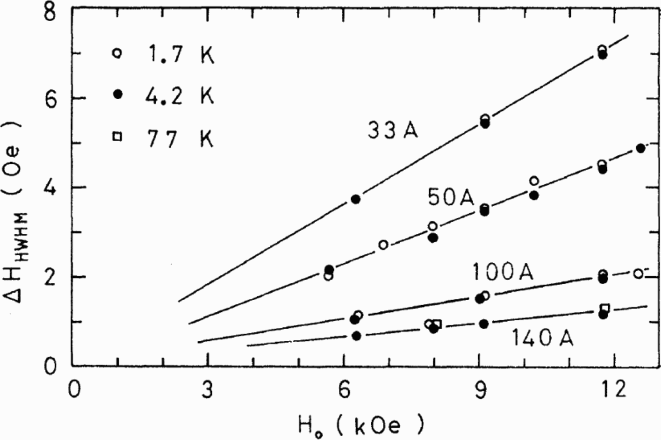
Measurements obtained by Yu et al. 87 showing how the half-width half-maximum of the main ¹⁹⁵Pt resonance peak varies as a function of particle diameter (in Å), applied magnetic field (H_o) and temperature (in K) (reprinted from Ref. 87 with permission: © 1980 American Physical Society)

Effect of particle size and temperature on the Knight shift

In general, the NMR spectrum for platinum nanoparticles consists of two peaks. One peak is at 1.138 G kHz^− 1, which is the same resonance observed in bulk platinum metal^94,95 and is therefore attributed to nuclei in a ‘bulk-like’ environment in the interior of the nanoparticle. The other at 1.100 G kHz^− 1 is attributed to nuclei on the surface.^84,96

Yano et al. measured the ¹⁹⁵Pt resonances on carbon-supported platinum nanoparticles ∼1–5 nm in diameter.⁹⁶ Their results in Fig. 7 clearly show these ‘surface’ and ‘bulk’ peaks. The intensity of a peak is proportional to the number of nuclei in that environment. Therefore, the smaller the nanoparticle, the larger the fraction of surface atoms and the higher the intensity of the surface peak at ∼1.100 G kHz^− 1. Similarly, the more atoms in the bulk-like interior of the nanoparticle, the larger the intensity of the bulk peak. Even small nanoparticles of 4.8 nm display significant bulk-like character. Conversely, in the smallest nanoparticles of 1.6 nm diameter, there is almost no evidence of any bulk-like behaviour except for some broadening in the surface peak, which suggests that even the few atoms in the interior of the nanoparticle are strongly influenced by those at the surface. The bulk peak present in the nanoparticles of diameter >2.6 nm varies with particle size, with the peak position tending to the bulk metal position of 1.138 G kHz^− 1 as the particle size increases. This would appear to contradict the previous conclusion by Yu et al. that the bulk peak position does not vary with diameter.^86,87 The majority of Yu et al.'s particles, however, were much larger than those studied by Yano et al., which suggests that the bulk peak tends to the bulk metal value in particles larger than ∼3–5 nm. Furthermore, Yano et al. observed hardly any change in the ‘surface peak’ position as a function of particle size. This implies that surface electronic properties are not affected by particle size (Fig. 7).

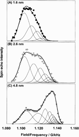
¹⁹⁵Pt NMR spectra for nanoparticles.⁹⁶ The symbols are the experimental intensities obtained from spin echo experiments on carbon-supported platinum nanoparticles. The thin solid lines are modelled resonances for individual layers and the thick solid lines are the sum of the thin solid lines to give an overall modelled NMR spectrum for each nanoparticle (reproduced from Ref. 96 with permission from the PCCP Owner Societies)

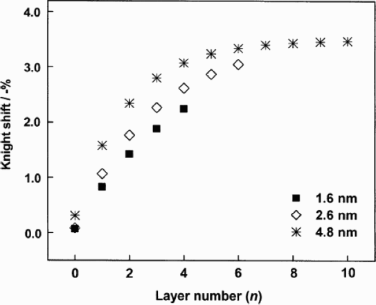
Calculated Knight shifts for each layer inside Pt nanoparticles using layer model analysis.⁹⁶ The surface layer is n = 0 (reproduced from Ref. 96 with permission from the PCCP Owner Societies)

Yu et al., to aid the interpretation of their line broadening experiments (see Fig. 6), tried to model the NMR absorption lines.^87,86 They assumed that the Knight shift only arose from s-electrons confined within a sphere acting as a free electron gas. The electron and electron spin densities were then calculated. The theoretical model showed good agreement to their experiments (see Fig. 9).

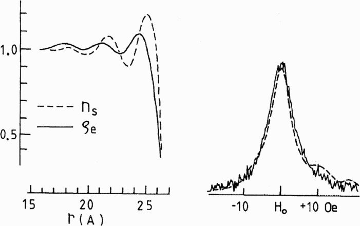
Left: calculated free electron charge density ρ_e and spin density n_s for a particle of radius, r, of 2.7 nm. Right: comparison between the corresponding calculated resonance peak (dashed line) and experimental peak (solid line). The experimental data correspond to a particle of 5 nm diameter measured at 10 kOe and 4.2 K (see Fig. 6)⁸⁷ (reprinted from Ref. 87 with permission: © 1980 American Physical Society)

Since the Knight shift for each atom is dependent on its local environment and is related to the electron density at the nucleus (equations (13) and (14)), an approximate NMR peak can be simulated by summing up the local density of states (LDOS) around all magnetic nuclei in the system. In 1993, Efetov and Prigodin employed the supersymmetry method to calculate these LDOS and thus the resonance peaks for nanoparticles independent of composition.⁹⁷ They found that the Knight shift decreased, while the broadening increased and became more asymmetric, with decreasing particle size and temperature.

In 1997, Pastawski and Gascón modelled NMR line shapes in particles, independent of composition.²⁶ They modelled the particles as cubes of atoms arranged in a simple cubic structure. The LDOS for the s-electrons within the layers of these cubes was then calculated using a tight-binding Hamiltonian. Adding the LDOS for the layers together produced a simulated NMR peak. They observed the same trends as Efetov and Prigodin, but additionally found that these trends broke down at very small diameters. In a later paper, Pastawski and Gascón concluded that the breakdown in trend was due to the large surface area/volume ratio of small particles and that the existence of ‘surface states’ would lead to large line broadenings.⁹⁸ This is consistent with the ‘surface peak’ apparent in experimental spectra of very small nanoparticles in the above sections. This approach was extended by Fritschij et al. 2 years later.⁹⁹

Yano et al.⁹⁶ and Tong et al.⁸⁴ used a layer model to simulate NMR spectra. They treated the nanoparticle as a set of concentric layers each in a cubo-octahedral arrangement. The NMR signal from each layer was then modelled as a Gaussian distribution. The sum of these Gaussians, weighted by the proportion of atoms in each layer, produced the simulated spectrum for the nanoparticle as a whole. In Fig. 8, the modelled spectra show good agreement to experiment. This shows that the Knight shift in the centre of the nanoparticle varies with particle size; however, the Knight shift of the surface atoms is independent of size. This implies that the surface states are not affected by those in the nanoparticle interior.

The electrons predominantly involved in the Knight shift are situated close to the Fermi level, E_f. Therefore, Yano et al.⁹⁶ concluded that resonance peak variation with size occurs as a result of the total change in the s- and d-like LDOS at E_f within each layer.

The hyperfine interaction can be expressed as the sum of positive s-like and negative d-like contributions.¹⁰⁰ In bulk Pt, the d-like hyperfine interaction is the dominant contribution to the Knight shift. However, in a nanoparticle, this d-like component decreases monotonically from the bulk-like centre to the surface.^101,102,96 Therefore, the Knight shift decreases from the centre to the surface of the nanoparticle and also decreases with decreasing particle size.^103–105

Effect of adsorbates on Knight shift

Tong et al. investigated how different adsorbates (ruthenium, hydrogen, carbon monoxide, cyanide, sulphur and oxygen) alter the ¹⁹⁵Pt Knight shift in pure platinum nanoparticles.⁸⁴ They found that the experimental surface peak was significantly shifted across a range of 11 000 ppm.

The adsorption of CO decreases the efficiency of platinum catalysts, particularly those in direct methanol fuel cells and hydrogen fuel cells. This CO ‘poisoning effect’¹⁰⁶ can be combated by alloying platinum (Pt) with ruthenium (Ru).^107–109

There are two proposed mechanisms for why Ru reduces the ‘poisoning effect’ of CO in Pt¹⁰⁶: (i)

Bifunctional mechanism—Ru promotes the creation of ‘oxygen-containing species’, which then react with the Pt–CO surface complex to oxidise the CO from the surface,

(ii)

Ligand field effect—Ru alters the electronic structure of Pt.

The Wieckowski group conclude from measuring the Knight shift in ¹⁹⁵Pt-NMR spectra¹⁰⁶ and infrared (IR) data¹¹⁰ that there are contributions from both mechanisms. The reasoning is as follows (see Fig. 10):

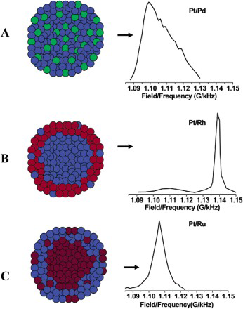
A selection of ¹⁹⁵Pt-NMR spectra for different platinum nanoparticle compositions along with representations of their atomic structure¹⁰⁶. The nanoparticles are 2–3 nm in diameter. Blue = Pt; green = Pd; red = Rh; brown = Ru (Figure and Spectrum C are reprinted from Ref. 106 with permission: © 2003 American Chemical Society; Spectrum A is reprinted from Ref. 111 with permission: © 1996 American Chemical Society; Spectrum B is reprinted from Ref. 112 with permission: © 1988 Royal Society of Chemistry)

(i)

The resonance peak in Pt nanoparticles (Pt-black) is subject to a large amount of broadening due to the range in Larmor frequencies from nuclei in the centre of the nanoparticle to those on the surface.

(ii)

The bulk Knight shift decreases with decreasing particle size. For example, the same group measured the bulk peak in 6 nm particles at 1.1322 G kHz^− 1, whereas for 2.8 nm nanoparticles, it was at 1.1306 G kHz^− 1.¹⁰⁶

(iii)

Alloyed nanoparticles consisting of a homogeneous solid solution tend to give broader peaks. However, if one of the elements clusters at the surface, then the peak becomes much sharper because there are a reduced number of nuclear environments. An example of homogeneous nanoparticle NMR spectra, in this case for a Pt–Pd nanoparticle, is shown in spectrum A in Fig. 10. Spectrum B in Fig. 10 shows a ¹⁹⁵Pt-NMR spectrum corresponding to Pt–Rh nanoparticles. The sharpness of the peak suggests clustering of Pt atoms. This peak is at 1.138 G kHz^− 1 (same as the bulk metal), which suggests that this cluster of Pt atoms must be in the centre of the nanoparticle. Therefore, the surface must be enriched with Rh. Spectrum C in Fig. 10 shows the ¹⁹⁵Pt resonance peak for Pt–Ru nanoparticles of 50–50 atomic composition. This is a fairly sharp peak, though not as sharp as in the Pt–Rh case. Assuming that the difference in elements does not affect the broadening, this suggests that there is a small degree of segregation (though not as much as in the Pt–Rh nanoparticle). The peak is situated at 1.104 G kHz^− 1. Since this is much smaller than the bulk value, this suggests that the surface is enriched with Pt atoms and that the Ru are mostly in the interior.

(iv)

These apparent changes in Knight shift as a function of Pt position suggest that the ligand field affect is a valid mechanism.

(v)

Additional IR spectra¹¹⁰ on ‘equivalent’ nanoparticles suggest that the Ru atoms on the surface are not evenly distributed but clustered. IR peaks were present for CO being adsorbed to Pt and also for CO being adsorbed to Ru. Thus, if there are regions of Ru on the surface, there must also exist boundaries between the Pt and Ru regions. These boundaries are necessary for the bifunctional mechanism.

(vi)

Overall, it can be deduced that the structures required for both mechanisms are present in the Pt–Ru nanoparticles. Therefore, it cannot be ruled out that both mechanisms are acting, though it cannot be said that they must necessarily both be acting.

¹⁹⁵Pt-NMR, along with a series of heat treatments, was used by Babu et al. on Pt–Ru nanoparticles to conclude that the efficiency of the oxidation of methanol can be raised by heat treating the nanoparticles to ∼200°C. This is because the heat treatment alters the composition of Ru on the nanoparticle surface.¹¹³

In addition to measuring ¹⁹⁵Pt resonances, ¹³C resonances from CO have been measured. These resonances also display a shift that appears to be related to the platinum Knight shift and can therefore be used to obtain information on the bonding environment and mobility of adsorbants on the nanoparticle surface. Babu et al. recorded ¹³C-NMR spectra for CO adsorbed onto the Pt–Ru nanoparticle surface.¹⁰⁶ This shift was smaller than that for CO adsorbed onto pure platinum nanoparticles (Pt-black). Kobayashi et al. used ¹³C NMR measurements to further investigate the role of CO on the surface of Pt nanoparticles.^114,115 This was continued by Babu et al.¹¹⁶ with the conclusion that the diffusion of CO on the nanoparticle surface is not the factor that limits the rate at which the nanoparticles catalyse the oxidation of methanol because the surface diffusion of CO is too fast.

There has been some research on how to control the size and shape of platinum nanoparticles since this can be used to tailor their properties. Ramirez et al. systematically investigated the effect of adding the weak ligand HDA (hexadecylamine) to stabilise the surface of the nanoparticle.⁸⁵ They recorded the different morphologies formed as a function of varying solvent concentrations of THF and toluene, carbon monoxide and H₂, and of changing which synthesis step involved the addition of HDA. They concluded that the strength at which the amine group in HDA bonded to the nanoparticle surface strongly influenced the final platinum morphology. The probability of coalescence is increased by weakening the bonding of the ligand to the surface of the nanoparticle and increasing the mobility of the amine group on the surface. This is because the HDA molecule undergoes a chemical exchange process on the Pt surface with bound (those bonded to the surface) and unbound (those in solution) HDA molecules switching places. This switching means that there are times when the surface is not passivated at all. At these times, the nanoparticles are more likely to bind to one another and thus coalesce. It was also hypothesised that the long chain of HDA molecules acted as a template to guide the nanoparticles into forming nanowires or nanorods.

In the same paper, Ramirez et al. also conducted some solution based ¹³C-NMR studies in order to investigate the bonding of the HDA (ligand) to the Pt nanoparticle surface.⁸⁵ A small shift of no more than 1 ppm was recorded in the peaks attributed to the three carbons closest to the amine group in HDA. Ramirez et al. suggested that this was due to the platinum Knight shift, on the basis that the same shift was not observed for HDA-passivated ruthenium and palladium nanoparticles.^117,118 This seems reasonable as it is likely that the HDA molecules are bonded to the nanoparticle surface via the amine group. Thus, these three carbons would be the closest to the platinum nuclei and would therefore experience the largest effect of the spin polarisation in the platinum via a series of hyperfine interactions. Furthermore, platinum Knight shifts are large, as mentioned earlier in this section. Therefore, it is possible that the platinum spin polarisation may affect neighbouring nuclei.

Conclusions

Hyperfine interactions manifest in a variety of materials with important applications, such as lithium intercalation materials for lithium-ion batteries and platinum nanoparticles for catalysis. Solid-state NMR spectra provide an excellent means for measuring these hyperfine interactions and thereby deducing the structure and properties of the materials. However, these experimental spectra are often difficult to interpret without the aid of first-principles calculations.

¹⁹⁵Pt-NMR spectra for platinum nanoparticles were simulated through a combination of LDOS and layer methods. For lithium intercalation materials, calculations of electron spin densities allowed the signs and approximate magnitude of hyperfine parameters to be estimated.⁴⁸ However, a fully quantatitive analysis could not be conducted due to the difficulty in accurately calculating the charge density at the nucleus. The calculation of hyperfine parameters was improved through the development of the PAW method.⁵² This allowed for the reconstruction of physically real valence wavefunctions at the nucleus. When used in conjunction with perturbation theory to calculate the effect of core polarisation on the core electrons, reasonable agreements to experiment were achieved for a set of small molecules and fullerene derivatives.^56,57,22 However, the accurate modelling of core polarisation has yet to be fully realised.

Acknowledgements

Thanks goes to J. R. Yates (University of Oxford) and B. J. Morgan (University of Bath) for their useful comments.

References

Pickard

C. J.

and Mauri

: ‘All-electron magnetic response with pseudopotentials: NMR chemical shifts’, Phys. Rev. B, 2001, 63, (24), 245101. doi: 10.1103/PhysRevB.63.245101

Yates

J. R.

, Pickard

C. J.

and Mauri

: ‘Calculation of NMR chemical shifts for extended systems using ultrasoft pseudopotentials’, Phys. Rev. B, 2007, 76, (2), 024401. doi: 10.1103/PhysRevB.76.024401

Joyce

S. A.

, Yates

J. R.

, Pickard

C. J.

and Mauri

: ‘A first principles theory of nuclear magnetic resonance J-coupling in solid-state systems’, J. Chem. Phys., 2007, 127, (20), 204107. doi: 10.1063/1.2801984

Bonhomme

, Gervais

, Babonneau

, Coelho

, Pourpoint

, Azas

, Ashbrook

S. E.

, Griffin

J. M.

, Yates

J. R.

, Mauri

and Pickard

C. J.

: ‘First-principles calculation of NMR parameters using the gauge including projector augmented wave method: a chemist's point of view’, Chem. Rev., 2012, 112, (11), 5733–5779. doi: 10.1021/cr300108a

Charpentier

: ‘The PAW/GIPAW approach for computing NMR parameters: a new dimension added to NMR study of solids’, Solid State Nucl. Magn. Reson., 2011, 40, (1), 1–20. doi: 10.1016/j.ssnmr.2011.04.006

Gerlach

and Stern

: ‘Das magnetische moment des silber-atoms’, Z. Phys., 1922, 9, (1), 353–355. doi: 10.1007/BF01326984

Frisch

and Stern

: ‘Über die magnetische ablenkung von wasser-stoffmoleklen und das magnetische moment des Protons. I’, Z. Phys., 1933, 85, (1-2), 4–16. doi: 10.1007/BF01330773

Estermann

and Stern

: ‘Über die magnetische ablenkung von wasser-stoffmoleklen und das magnetische moment des protons. II’, Z. Phys., 1933, 85, (1-2), 17–24. doi: 10.1007/BF01330774

Estermann

and Stern

: ‘Über die magnetische ablenkung von isotopen wasserstoffmoleklen und das magnetische moment des “Deutons”’, Z. Phys., 1933, 86, (1–2), 132–134. doi: 10.1007/BF01340190

10.

Estermann

, Simpson

and Stern

: ‘The magnetic moment of the proton’, Phys. Rev., 1937, 52, (6), 535–545. doi: 10.1103/PhysRev.52.535

11.

Gorter

C. J.

: ‘Negative result of an attempt to detect nuclear magnetic spins’, Physica, 1936, 3, (9), 995–998. doi: 10.1016/S0031-8914(36)80324-3

12.

Rabi

, Zacharias

, Millman

and Kusch

: ‘A new method of measuring nuclear magnetic moment’, Phys. Rev., 1938, 53, (4), 318. doi: 10.1103/PhysRev.53.318

13.

Rabi

, Millman

, Kusch

and Zacharias

: ‘The molecular beam resonance method for measuring nuclear magnetic moments. The magnetic moments of ₃Li⁶, ₃Li⁷ and ₉F^19’, Phys. Rev., 1939, 55, (6), 526–535. doi: 10.1103/PhysRev.55.526

14.

Nobel Media AB 2013 . All Nobel prizes in physics. http://www. nobelprize.org/nobel_prizes/physics/laureates/.

15.

Ramsey

N. F.

: ‘Early history of magnetic resonance’, Bull. Magn. Reson., 1985, 7, 94.

16.

Hurwitz

: ‘Milestones in magnetic resonance: a new method of measuring nuclear magnetic moment’, J. Magn. Reson. Imaging, 1992, 2, (2), 131–133. doi: 10.1002/jmri.1880020203

17.

Hore

P. J.

: ‘Oxford chemistry primers—nuclear magnetic resonance’, 1995, Oxford, Oxford University Press.

18.

Harris

R. K.

, Apperley

D. C.

and Hodgkinson

: ‘Solid state NMR: basic principles & practice’, 2012, New York, Momentum Press.

19.

Foot

C. J.

: ‘Atomic physics’, 2011, Oxford, Oxford University Press.

20.

Neese

: ‘Metal and ligand hyperfine couplings in transition metal complexes: the effect of spin-orbit coupling as studied by coupled perturbed Kohn-Sham theory’, J. Chem. Phys., 2003, 118, (9), 3939R–3948R. doi: 10.1063/1.1540619

21.

Arbuznikov

A. V.

, Vaara

and Kaupp

: ‘Relativistic spin-orbit effects on hyperfine coupling tensors by density-functional theory’, J. Chem. Phys., 2004, 120, (5), 2127–2139. doi: 10.1063/1.1636720

22.

Filidou

, Ceresoli

, Morton

J. J. L.

and Giustino

: ‘First-principles investigation of hyperfine interactions for nuclear spin entanglement in photo excited fullerenes’, Phys. Rev. B, 2012, 85, (11), 115430. doi: 10.1103/PhysRevB.85.115430

23.

Atkins

and Friedman

: ‘Molecular quantum mechanics’, 2005, Oxford, Oxford University Press.

24.

Knight

: ‘Nuclear magnetic resonance shift in metals’, Phys. Rev., 1949, 76, (8), 1259–1260. doi: 10.1103/PhysRev.76.1259.2

25.

Kittel

: ‘Introduction to solid state physics’, 1986, New York, John Wiley & Sons Inc.

26.

Pastawski

and Gascón

: ‘NMR line shape in metallic nanoparticles: a matrix continued fractions evaluation’, Phys. Rev., 1997, 56, (8), 4887–4892. doi: 10.1103/PhysRevB.56.4887

27.

Y. Q.

, Malon

, Martineau

, Taulelle

and Nishiyama

: ‘Rapid measurement of multidimensional ¹H solid-state NMR spectra at ultra-fast MAS frequencies’, J. Magn. Reson., 2014, 239, 75–80. doi: 10.1016/j.jmr.2013.12.010

28.

Martin

R. M.

: ‘Electronic structure: basic theory and practical methods’, 2010, Cambridge, Cambridge University Press.

29.

Koch

and Holthausen

M. C.

: ‘A chemist's guide to density functional theory’, 2000, Weinheim, Wiley-VCH.

30.

Hohenberg

and Kohn

: ‘Inhomogeneous electron gas’, Phys. Rev. B, 1964, 136, (3B), B864. doi: 10.1103/PhysRev.136.B864

31.

Kohn

and Sham

L. J.

: ‘Self-consistent equations including exchange and correlation effects’, Phys. Rev., 1965, 140, (4A), 1133. doi: 10.1103/PhysRev.140.A1133

32.

Ceperley

D. M.

and Alder

B. J.

: ‘Ground state of the electron gas by a stochastic method’, Phys. Rev. Lett., 1980, 45, (7), 566–569. doi: 10.1103/PhysRevLett.45.566

33.

Perdew

J. P.

and Zunger

: ‘Self-interaction correction to density functional approximations for many-electron systems’, Phys. Rev. B, 1981, 23, (10), 5048–5079. doi: 10.1103/PhysRevB.23.5048

34.

Perdew

J. P.

, Burke

and Ernzerhof

: ‘Generalized gradient approximation made simple’, Phys. Rev. Lett., 1996, 77, 3865–3868. doi: 10.1103/PhysRevLett.77.3865

35.

Dovesi

, Orlando

, Civalleri

, Roetti

, Saunders

V. R.

and Zicovich-Wilson

C. M.

: ‘CRYSTAL: a computational tool for the ab initio study of the electronic properties of crystals’, Z. Kristallogr., 2005, 220, (5–6), 571–573.

36.

Soler

J. M.

, Artacho

, Gale

J. D.

, García

, Junquera

, Ordejón

and Sánchez-Portal

: ‘The SIESTA method for ab initio order-N materials simulation’, J. Phys. Condens. Matter, 2002, 14, (11), 2745–2779. doi: 10.1088/0953-8984/14/11/302

37.

Clark

S. J.

, Segall

M. D.

, Pickard

C. J.

, Hasnip

P. J.

, Probert

M. J.

, Refson

and Payne

M. C.

: ‘First principles methods using CASTEP’, Z. Kristall., 2005, 220, (5-6), 567–570.

38.

Monkhorst

H. J.

and Pack

J. D.

: ‘Special points for Brillouin-zone integration’, Phys. Rev. B, 1976, 13, 5188. doi: 10.1103/PhysRevB.13.5188

39.

Methfessel

and Paxton

: ‘High-precision sampling for Brillouin-zone integration in metals’, Phys. Rev. B, 1989, 40, (6), 3616–3621. doi: 10.1103/PhysRevB.40.3616

40.

de Gironcoli

: ‘Lattice dynamics of metals from density-functional perturbation theory’, Phys. Rev. B, 1995, 51, 6773–6776. doi: 10.1103/PhysRevB.51.6773

41.

d'Avezac

, Marzari

and Mauri

: ‘Spin and orbital magnetic response in metals: susceptibility and NMR shifts’, Phys. Rev. B, 2007, 76, (16), 165122. doi: 10.1103/PhysRevB.76.165122

42.

Ramsey

: ‘The internal diamagnetic field correction in measurements of the proton magnetic moment’, Phys. Rev., 1950, 77, (4), 567. doi: 10.1103/PhysRev.77.567

43.

Ramsey

: ‘Magnetic shielding of nuclei in molecules’, Phys. Rev., 1950, 78, (6), 699–703. doi: 10.1103/PhysRev.78.699

44.

Ramsey

: ‘Electron coupled interactions between nuclear spins in molecules’, Phys. Rev., 1953, 91, (2), 303–307. doi: 10.1103/PhysRev.91.303

45.

Heise

, Köhler

F. H.

, Mota

, Novoa

J. J.

and Veciana

: ‘Determination of the spin distribution in nitronylnitroxides by solid-state ¹., ²H, and ¹³C NMR spectroscopy’, J. Am. Chem. Soc., 1999, 121, (41), 9659–9667. doi: 10.1021/ja991188t

46.

Maruta

, Takeda

, Imachi

, Ishida

, Nogami

and Yamaguchi

: ‘Solid-state high-resolution ¹H and ²D NMR study of the electron spin density distribution of the hydrogen-bonded organic ferromagnetic compound 4-hydroxyimino-TEMPO’, J. Am. Chem. Soc., 1999, 121, (2), 424–431. doi: 10.1021/ja982393w

47.

Köhler

, Seifert

, Gerstmann

, Elstner

, Overhof

and Frauenheim

Th.

: ‘Approximate density-functional calculations of spin densities in large molecular systems and complex solids’, Phys. Chem. Chem. Phys., 2001, 3, (23), 5109–5114. doi: 10.1039/b105782k

48.

Carlier

, Ménétrier

, Grey

C. P.

, Delmas

and Ceder

: ‘Understanding the NMR shifts in paramagnetic transition metal oxides using density functional theory calculations’, Phys. Rev. B, 2003, 67, (17), 174103. doi: 10.1103/PhysRevB.67.174103

49.

Ban

, Rankin

K. N.

, Gauld

J. W.

and Boyd

R. J.

: ‘Recent applications of density functional theory calculations to biomolecules’, Theor. Chem. Acc., 2002, 108, (1), 1–11. doi: 10.1007/s00214-002-0344-z

50.

Neese

: ‘Quantum chemical calculations of spectroscopic properties of metalloproteins and model compounds: EPR and Mössbauer properties’, Curr. Opin. Chem. Biol., 2003, 7, (1), 125–135. doi: 10.1016/S1367-5931(02)00006-6

51.

Kaupp

and Köhler

F. H.

: ‘Combining NMR spectroscopy and quantum chemistry as tools to quantify spin density distributions in molecular magnetic compounds’, Coord. Chem. Rev., 2009, 253, (1920), 2376–2386. doi: 10.1016/j.ccr.2008.12.020

52.

Van de Walle

C. G.

and Blöchl

P. E.

: ‘First principles calculations of hyperfine parameters’, Phys. Rev. B, 1993, 47, (8), 4244–4255. doi: 10.1103/PhysRevB.47.4244

53.

Yates

J. R.

: ‘Prediction of NMR J-coupling in solids with the planewave pseudopotential approach’, Magn. Reson. Chem., 2010, 48, (S1), S23–S31. doi: 10.1002/mrc.2646

54.

Yazyev

O. V.

, Tavernelli

, Helm

and Rothlisberger

: ‘Core spin-polarization correction in pseudopotential-based electronic structure calculations’, Phys. Rev. B, 2005, 71, (11), 115110. doi: 10.1103/PhysRevB.71.115110

55.

Declerck

, Pauwels

, Van Speybroeck

and Waroquier

: ‘First-principles calculations of hyperfine parameters with the Gaussian and augmented-plane-wave method: application to radicals embedded in a crystalline environment’, Phys. Rev. B, 2006, 74, (24), 245103. doi: 10.1103/PhysRevB.74.245103

56.

Bahramy

M. S.

, Sluiter

M. H. F.

and Kawazoe

: ‘First-principles calculations of hyperfine parameters with the all-electron mixed-basis method’, Phys. Rev. B, 2006, 73, (4), 045111. doi: 10.1103/PhysRevB.73.045111

57.

Bahramy

M. S.

, Sluiter

M. H. F.

and Kawazoe

: ‘Pseudopotential hyperfine calculations through perturbative core-level polarization’, Phys. Rev. B, 2007, 76, (3), 035124. doi: 10.1103/PhysRevB.76.035124

58.

Stanley Whittingham

: ‘Lithium batteries and cathode materials’, Chem. Rev., 2004, 104, (10), 4271–4302. doi: 10.1021/cr020731c

59.

Grey

C. P.

and Lee

Y. J.

: ‘Lithium MAS NMR studies of cathode materials for lithium-ion batteries’, Solid State Sci., 2003, 5, (6), 883–894. doi: 10.1016/S1293-2558(03)00113-4

60.

Grey

C. P.

and Dupré

: ‘NMR studies of cathode materials for lithium-ion rechargeable batteries’, Chem. Rev., 2004, 104, (10), 4493–4512. doi: 10.1021/cr020734p

61.

Marichal

, Hirschinger

, Granger

, Ménétrier

, Rougier

and Delmas

: ‘⁶Li and ⁷Li NMR in the LiNi_1 − yCo^yO₂ solid solution (0 ≤ y ≤ 1)’, Inorg. Chem., 1995, 34, (7), 1773–1778. doi: 10.1021/ic00111a026

62.

Alcántara

, Lavela

, Relaño

P. L.

, Tirado

J. L.

, Zhecheva

and Stoyanova

: ‘X-ray diffraction, EPR, and ⁶Li and ²⁷Al MAS NMR study of LiAlO₂–LiCoO₂ solid solutions’, Inorg. Chem., 1998, 37, (2), 264–269. doi: 10.1021/ic9707220

63.

Peeters

M. P. J.

, van Bommel

M. J.

, Neilen-ten Wolde

P. M. C.

, van Hal

H. A. M.

, Keur

W. C.

and Kentgens

A. P. M.

: ‘A ⁶Li, ⁷Li and ⁵⁹Co MAS NMR study of rock salt type Li_xCoO₂ (0.48 ≤ × ≤ 1.05)’, Solid State Ionics, 1998, 112, (1–2), 41–52. doi: 10.1016/S0167-2738(98)00213-6

64.

Levasseur

, Ménétrier

, Suard

and Delmas

: ‘Evidence for structural defects in non-stoichiometric HT-LiCoO₂: electrochemical, electronic properties and ⁷Li NMR studies’, Solid State Ionics, 2000, 128, (1–4), 11–24. doi: 10.1016/S0167-2738(99)00335-5

65.

Carlier

, Ménétrier

and Delmas

: ‘⁷Li MAS NMR study of electrochemically deintercalated Li_xNi_0.30Co_0.70O₂ phases: evidence of electronic and ionic mobility, and redox processes’, J. Mater. Chem., 2001, 11, (2), 594–603. doi: 10.1039/b006179o

66.

Pan

, Lee

Y. J.

, Ammundsen

and Grey

C. P.

: ‘⁶Li MAS NMR studies of the local structure and electrochemical properties of Cr-doped lithium manganese and lithium cobalt oxide cathode materials for lithium-ion batteries’, Chem. Mater., 2002, 14, (5), 2289–2299. doi: 10.1021/cm011623u

67.

Lee

Y. J.

and Grey

C. P.

: ‘⁶Li magic-angle spinning (MAS) NMR study of electron correlations, magnetic ordering, and stability of lithium manganese(III) oxides’, Chem. Mater., 2000, 12, (12), 3871–3878. doi: 10.1021/cm000469t

68.

Delmas

, Fouassier

and Hagenmuller

: ‘Structural classification and properties of the layered oxides’, Physica B+C, 1980, 99, (1–4), 81–85. doi: 10.1016/0378-4363(80)90214-4

69.

Mustarelli

, Massarotti

, Bini

and Capsoni

: ‘Transferred hyperfine interaction and structure in LiMn₂O₄ and Li₂MnO₃ coexisting phases: a XRD and ⁷Li NMR-MAS study’, Phys. Rev. B, 1997, 55, (18), 12018–12024. doi: 10.1103/PhysRevB.55.12018

70.

Morgan

K. R.

, Collier

, Burns

and Ooi

: ‘A ⁶Li and ⁷Li MAS NMR study of the spinel-type manganese oxide LiMn₂O₄ and the rock salt-type manganese oxide Li₂MnO₃’, J. Chem. Soc. Chem. Commun., 1994, (14), 1719. doi: 10.1039/c39940001719

71.

Gee

, Horne

C. R.

, Cairns

E. J.

and Reimer

J. A.

: ‘Supertransferred hyperfine fields at ⁷Li: variable temperature ⁷Li NMR studies of LiMn₂O₄-based spinels’, J. Phys. Chem. B, 1998, 102, (50), 10142–10149. doi: 10.1021/jp982301p

72.

Lee

Y. J.

, Wang

and Grey

C. P.

: ‘⁶Li and ⁷Li MAS NMR studies of lithium manganate cathode materials’, J. Am. Chem. Soc., 1998, 120, (48), 12601–12613. doi: 10.1021/ja9817794

73.

Tucker

M. C.

, Doeff

M. M.

, Richardson

T. J.

, Finones

, Reimer

J. A.

and Cairns

E. J.

: ‘⁷Li and ³¹P magic angle spinning nuclear magnetic resonance of LiFePO₄-type materials’, Electrochem. Solid-State Lett., 2002, 5, (5), A95. doi: 10.1149/1.1464505

74.

Tucker

M. C.

, Doeff

M. M.

, Richardson

T. J.

, Fiñones

, Cairns

E. J.

and Reimer

J. A.

: ‘Hyperfine fields at the Li site in LiFePO₄-type olivine materials for lithium rechargeable batteries: a ⁷Li MAS NMR and SQUID study’, J. Am. Chem. Soc., 2002, 124, (15), 3832–3833. doi: 10.1021/ja017838m

75.

Ganguly

, Venkatraman

T. N.

, Pradhan

, Rajamohanan

P. R.

and Ganapathy

: ‘Environment dependence of metal or ligand oxidation in copper oxide systems: evidence from heats of formation and ⁷Li solid state NMR studies’, J. Phys. Chem., 1996, 100, (12), 5017–5024. doi: 10.1021/jp952770g

76.

Burley

J. C.

, Battle

P. D.

, Gallon

D. J.

, Sloan

, Grey

C. P.

and Rosseinsky

M. J.

: ‘Magnetism and structural chemistry of the n = 1 Ruddlesden–Popper phases La₄LiMnO₈ and La₃SrLiMnO₈’, J. Am. Chem. Soc., 2002, 124, (4), 620–628. doi: 10.1021/ja012023z

77.

Shannon

R. D.

and Prewitt

C. T.

: ‘Effective ionic radii in oxides and fluorides’, Acta Crystallogr., 1969, 25, (5), 925–946. doi: 10.1107/S0567740869003220

78.

Clement

R. J.

, Pell

A. J.

, Middlemiss

D. S.

, Strobridge

F. C.

, Miller

J. K.

, Whittingham

M. S.

, Emsley

, Grey

C. P.

and Pintacuda

: ‘Spin-transfer pathways in paramagnetic lithium transition-metal phosphates from combined broadband isotropic solid-state MAS NMR spectroscopy and DFT calculations’, J. Am. Chem. Soc., 2012, 134, (41), 17178–17185. doi: 10.1021/ja306876u

79.

Middlemiss

D. S.

, Ilott

A. J.

, Clément

R. J.

, Strobridge

F. C.

and Grey

C. P.

: ‘Density functional theory-based bond pathway decompositions of hyperfine shifts: equipping solid-state NMR to characterize atomic environments in paramagnetic materials’, Chem. Mater., 2013, 25, (9), 1723–1734. doi: 10.1021/cm400201t

80.

Mali

, Sirisopanaporn

, Masquelier

, Hanzel

and Dominko

: ‘Li₂FeSiO₄ polymorphs probed by ⁶Li MAS NMR and ⁵⁷Fe Mössbauer spectroscopy’, Chem. Mater., 2011, 23, (11), 2735–2744. doi: 10.1021/cm103193a

81.

Iggo

J. A.

: ‘Oxford chemistry primers—NMR spectroscopy in inorganic chemistry’, 1999, Oxford, Oxford University Press.

82.

Halperin

: ‘Quantum size effects in metal particles’, Rev. Mod. Phys., 1986, 58, (3), 533–606. doi: 10.1103/RevModPhys.58.533

83.

Butterworth

: ‘Nuclear magnetic relaxation and shift in platinum’, Phys. Rev. Lett., 1962, 8, (11), 423–424. doi: 10.1103/PhysRevLett.8.423

84.

Tong

, Rice

, Wieckowski

and Oldfield

: ‘¹⁹⁵ Pt-NMR of platinum electrocatalysts: Friedel-Heine invariance and correlations between platinum Knight shifts, healing length, and adsorbate electronegativity’, J. Am. Chem. Soc., 2000, 122, (48), 11921–11924. doi: 10.1021/ja002254q

85.

Ramirez

, Eradès

, Philippot

, Lecante

and Chaudret

: ‘Shape control of platinum nanoparticles’, Adv. Funct. Mater., 2007, 17, (13), 2219–2228. doi: 10.1002/adfm.200600633

86.

and Halperin

W. P.

: ‘The microelectronic structure of platinum particles investigated by NMR’, J. Low Temp. Phys., 1981, 45, (1–2), 189–232. doi: 10.1007/BF00661149

87.

, Gibson

, Hunt

and Halperin

: ‘Observation of conduction-electron density oscillations at the surface of platinum particles’, Phys. Rev. Lett., 1980, 44, (5), 348–351. doi: 10.1103/PhysRevLett.44.348

88.

Slichter

C. P.

: ‘NMR study of platinum catalysts’, Surf. Sci., 1981, 106, (1), 382–396. doi: 10.1016/0039-6028(81)90226-0

89.

Slichter

C. P.

: ‘NMR study of platinum catalysts’, Surf. Sci. Lett., 1981, 106, (1), A180–A181. doi: 10.1016/0167-2584(81)90351-0

90.

Stokes

, Rhodes

, Wang

P.-K.

, Slichter

and Sinfelt

: ‘NMR of platinum catalysts. III. Microscopic variation of the Knight shifts’, Phys. Rev., 1982, 26, (7), 3575–3581. doi: 10.1103/PhysRevB.26.3575

91.

Rhodes

, Wang

P.-K.

, Makowka

, Rudaz

, Stokes

and Slichter

and Sinfelt

: ‘NMR of platinum catalysts. II. Relaxation’, Phys. Rev., 1982, 26, (7), 3569–3574. doi: 10.1103/PhysRevB.26.3569

92.

Rhodes

, Wang

P.-K.

, Stokes

, Slichter

and Sinfelt

: ‘NMR of platinum catalysts. I. Line shapes’, Phys. Rev. B, 1982, 26, (7), 3559–3568. doi: 10.1103/PhysRevB.26.3559

93.

van der Klink

, Buttet

and Graetzel

: ‘Knight shift in small platinum particles’, Phys. Rev. B, 1984, 29, (11), 6352–6355. doi: 10.1103/PhysRevB.29.6352

94.

Belrose

, Wieckowski

and Oldfield

: ‘First observation of platinum-195 nuclear magnetic resonance in commercial graphite-supported platinum electrodes in an electrochemical environment’, J. Am. Chem. Soc., 1997, 119, (48), 11709–11710. doi: 10.1021/ja970866d

95.

Slichter

C. P.

: ‘Probing phenomena at metal surfaces by NMR’, Annu. Rev. Phys. Chem., 1986, 37, 25–51. doi: 10.1146/annurev.pc.37.100186.000325

96.

Yano

, Inukai

, Uchida

, Watanabe

, Babu

P. K.

, Kobayashi

, Chung

J. H.

, Oldfield

and Wieckowski

: ‘Particle-size effect of nanoscale platinum catalysts in oxygen reduction reaction: an electrochemical and ¹⁹⁵Pt EC-NMR study’, Phys. Chem. Chem. Phys., 2006, 8, (42), 4932–4939. doi: 10.1039/b610573d

97.

Efetov

and Prigodin

: ‘Local density of states distribution and NMR in small metallic particles’, Phys. Rev. Lett., 1993, 70, (9), 1315–1318. doi: 10.1103/PhysRevLett.70.1315

98.

Gascón

J. A.

and Pastawski

H. M.

: ‘Surface effects on the statistics of the local density of states in metallic nanoparticles: manifestation on the NMR spectra’, Mod. Phys. Lett. B, 2005, 19, (25), 1285–1294. doi: 10.1142/S0217984905009250

99.

Fritschij

, Brom

, de Jongh

and Schmid

: ‘Mesoscopic fluctuations in small metal particles studied by nuclear magnetic resonance’, Phys. Rev. Lett., 1999, 82, (10), 2167–2170. doi: 10.1103/PhysRevLett.82.2167

100.

Yafet

and Jaccarino

: ‘Nuclear spin relaxation in transition metals; core polarization’, Phys. Rev., 1964, 133, (6A), A1630–A1637. doi: 10.1103/PhysRev.133.A1630

101.

Weinert

and Freeman

: ‘Relativistic spin polarization and magnetization: Knight shift of Pt(001)’, Phys. Rev. B, 1983, 28, (11), 6262–6269. doi: 10.1103/PhysRevB.28.6262

102.

Bucher

J. P.

, Buttet

, Van Der Klink

J. J.

and Graetzel

: ‘Electronic properties and local densities of states in clean and hydrogen covered Pt particles’, Surf. Sci., 1989, 214, (3), 347–357. doi: 10.1016/0039-6028(89)90175-1

103.

van der Klink

J. J.

: ‘A local-density formulation for NMR parameters in metals’, J. Phys. Condens. Matter, 1996, 8, (11), 1845–1850. doi: 10.1088/0953-8984/8/11/026

104.

Rice

, Tong

, Oldfield

and Wieckowski

: ‘Cyclic voltammetry and ¹⁹⁵Pt nuclear magnetic resonance characterization of graphite-supported commercial fuel cell grade platinum electrocatalysts’, Electrochim. Acta, 1998, 43, (19), 2825–2830. doi: 10.1016/S0013-4686(98)00023-1

105.

Rice

, Godbout

, Wieckowski

and Oldfield

: ‘Correlation between the Knight shift of chemisorbed CO and the Fermi level local density of states at clean platinum catalyst surfaces’, J. Am. Chem. Soc., 1999, 121, (13), 2996–3003. doi: 10.1021/ja9830492

106.

Babu

P. K.

, Kim

H. S.

, Oldfield

and Wieckowski

: ‘Electronic alterations caused by ruthenium in PtRu alloy nanoparticles as revealed by electrochemical NMR’, J. Phys. Chem. B, 2003, 107, (31), 7595–7600. doi: 10.1021/jp022679u

107.

Marković

N. M.

, Gasteiger

H. A.

, Ross

P. N.

, Jiang

, Villegas

and Weaver

M. J.

: ‘Electro-oxidation mechanisms of methanol and formic acid on Pt–Ru alloy surfaces’, Electrochim. Acta, 1995, 40, (1), 91–98. doi: 10.1016/0013-4686(94)00241-R

108.

Frelink

, Visscher

and van Veen

J. A. R.

: ‘Measurement of the Ru surface content of electrocodeposited PtRu electrodes with the electrochemical quartz crystal microbalance: implications for methanol and CO electrooxidation’, Langmuir, 1996, 12, (15), 3702–3708. doi: 10.1021/la9502709

109.

Waszczuk

, Solla-Gullón

, Kim

H.-S.

, Tong

Y. Y.

, Montiel

, Aldaz

and Wieckowski

: ‘Methanol electrooxidation on platinum/ruthenium nanoparticle catalysts’, J. Catal., 2001, 203, (1), 1–6. doi: 10.1006/jcat.2001.3389

110.

Park

, Wieckowski

and Weaver

M. J.

: ‘Electrochemical infrared characterization of CO domains on ruthenium-decorated platinum nanoparticles’, J. Am. Chem. Soc., 2003, 125, (8), 2282–2290. doi: 10.1021/ja028154x

111.

Tong

Y. Y.

, Yonezawa

, Toshima

and van der Klink

J. J.

: ‘¹⁹⁵Pt-NMR of polymer-protected Pt/Pd bimetallic catalysts’, J. Phys. Chem., 1996, 100, (2), 730–733. doi: 10.1021/jp951656v

112.

Wang

, Ansermet

J.-P.

, Slichter

C. P.

and Sinfelt

J. H.

: ‘Nuclear magnetic resonance study of Pt–Rh bimetallic clusters’, J. Chem. Soc., Faraday Trans., 1988, 84, (11), 3785. doi: 10.1039/f19888403785

113.

Babu

P. K.

, Kim

H. S.

, Kuk

S. T.

, Chung

J. H.

, Oldfield

, Wieckowski

and Smotkin

E. S.

: ‘Activation of nanoparticle Pt–Ru fuel cell catalysts by heat treatment: a ¹⁹⁵Pt NMR and electrochemical study’, J. Phys. Chem. B, 2005, 109, (36), 17192–17196. doi: 10.1021/jp058138x

114.

Kobayashi

, Babu

P. K.

, Gancs

, Chung

J. H.

, Oldfield

and Wieckowski

: ‘An NMR determination of CO diffusion on platinum electrocatalysts’, J. Am. Chem. Soc., 2005, 127, (41), 14164–14165. doi: 10.1021/ja0550475

115.

Kobayashi

, Babu

P. K.

, Chung

J. H.

, Oldfield

and Wieckowski

: ‘Coverage dependence of CO surface diffusion on Pt nanoparticles: an EC-NMR study’, J. Phys. Chem. C, 2007, 111, (19), 7078–7083. doi: 10.1021/jp066803b

116.

Babu

P. K.

, Chung

J.-H.

, Oldfield

and Wieckowski

: ‘CO surface diffusion on platinum fuel cell catalysts by electrochemical NMR’, Electrochim. Acta, 2008, 53, (23), 6672–6679. doi: 10.1016/j.electacta.2008.02.046

117.

Pan

, Pelzer

, Philippot

, Chaudret

, Dassenoy

, Lecante

and Casanove

M.-J.

: ‘Ligand-stabilized ruthenium nanoparticles: synthesis, organization, and dynamics’, J. Am. Chem. Soc., 2001, 123, (31), 7584–7593. doi: 10.1021/ja003961m

118.

Ramirez

, Jansat

, Philippot

, Lecante

, Gomez

, Masdeu-Bultó

A. M.

and Chaudret

: ‘Influence of organic ligands on the stabilization of palladium nanoparticles’, J. Organomet. Chem., 2004, 689, (24), 4601–4610. doi: 10.1016/j.jorganchem.2004.09.006