
Abstract
Strategic planning in mining is an important value accretive process. One of the most essential aspects during the planning phase is determining the correct system design. A traditional mine design process develops a fixed system for one set of conditions or expected values. An alternative is to develop a robust system that deals with variation, by handling a range of conditions within the optimisation process. Conversely, a flexible design can be generated which changes the system dynamically over time in response to change. It is hypothesised that a flexible design generates more value than a robust design which in turn generates more value than a traditional design. However, due to constant change, a fully flexible design is not practical. Ideally, a hybrid of the two methods would be optimal. An operational design is proposed as a manual solution to this problem. This paper compares these different new design methodologies.
Introduction
Decision making in mining operations can take many years due to the period of time required to explore and develop a large deposit. During the study and construction period, many uncertainties can unfold and multiple economic cycles may occur. Making decisions based on single point estimates of the future limits flexibility, potentially resulting in premature foreclosure of an operation. By considering changing conditions (both upwards and downwards movements) in the decision making process, a company is able to include flexibility in an operation allowing value to be maximised. Current methodologies impair a decision maker's ability to justify this additional flexibility.
Building flexibility into an operation provides a company with the ability to quickly respond to change; however, flexibility comes at a price. For example, an operation of building a crusher to feed a processing plant has an initial plan to produce at 6 Mtpa. An option exists to build the allowance for a plant expansion to 8 Mtpa (by increasing the size of the foundations and footings to allow physical room for larger equipment). However, when the decision to build the plant is made, to minimise initial capital investment, this flexibility is removed. One year into the operation, the sale price of the product doubles and costs slightly increase, while all other variables hold. In this environment, it is considered favourable to expand the operation; however, due to the cost cutting decision, this flexibility was removed from the plant and to make the matter worse, production needs to be maintained so the only option is to build a new crusher. Unfortunately, this will come at a significant capital cost and time to build; reducing the overall value of the operation had this flexibility initially been incorporated. This upfront flexibility is difficult to justify with current decision making tools. Advances in an area broadly known as real options ‘in’ projects (ROIP) are beginning to address this gap (de Neufville et al., 2005; de Neufville, 2006; Wang and de Neufville, 2005, 2006; Cardin et al., 2008; Groeneveld et al., 2009).
Real options ‘in’ projects are located midway between financial real options analysis (which does not deal with engineering system flexibility) and traditional engineering approaches (which do not deal with financial flexibility). An analysis done using ROIP methods allows the design of a system under uncertainty to be studied. Through the analysis process, the value of each design option can be tested. Having this information allows the decision maker to make an informed decision on what flexibility to incorporate in the final design.
Previous papers using ROIP methods have shown the value of this technique (Cardin et al., 2008; Groeneveld et al., 2009; Groeneveld and Topal, 2011). Cardin et al. (2008) implemented this technique for mining projects with a Chilean mine in the ‘Cluster Toki’ region. In the paper, a methodology is implemented where operating plans are varied by truck fleet capacity and crusher size in response to changing prices. For each price scenario, the optimal operational plan is selected. The application of this method resulted in ∼30% more project value than current estimates. This paper provides a strong basis on which to grow ROIP theory in mining. Though there are several deficiencies in the model. The approach limits the flexibility by only including a handful of static operational plans; it assumes that the schedule of material moved is fixed, fails to deal with variation in ore grade and recovery and fails to consider options in the main value adding stages of a mining operation.
Groeneveld et al. (2009) outlined a methodology for determining a flexible mine design by dynamically including design options in the optimisation in order to maximise value. Multiple ‘states of the world’ were simulated and the optimal design for each state was determined. A dataset of results was formed from the output of each simulated scenario. From this dataset, a cumulative probability graph was produced, commonly known as a value at risk graph. This resulting curve represents a theoretical maximum achievable value. However, this assumes that a decision maker can make perfect decisions. In reality, this is impracticable.
An alternative is to produce a single fixed design which handles optimally handles change. This is achieved by taking the full set of uncertainties into the optimisation and developing a fixed design that optimally handles the changing uncertainties. The resultant design would be a robust design as it would best handle variation. Since the optimisation includes high price and low price scenarios, it will attempt to produce a design that minimises any losses and maximise any potential upside, while considering that these are extreme scenarios and the main scenarios are around the average. Note that this design is fundamentally different to a design just generated based on the average value and this will be shown in the illustrative case study.
However, a robust design proposes that a ‘set and watch’ approach is taken by management. Therefore, it fails to value active management of an operation. So, a flexible model proposes constant change which is not practicable and a robust model does not allow management decisions. To overcome these limitations, it is proposed that an operational design be generated where the initial periods have a fixed ‘robust’ design and the later years have a flexible design where management has the ability to have multiple options in the pipeline.
This paper compares these different design methodologies. A summary of the methodology used for generating the designs is outlined followed by the mathematical formulation of the robust design under uncertainty, using mixed integer programming (MIP) and Monte Carlo simulation (MCS) techniques. Furthermore, an operational design is proposed as a solution to the limitations of the robust and flexible design methodologies. Finally, the different design methodologies are compared against each other and a traditional design approach, in an illustrative case study.
Methodology
It is proposed that for these different design scenarios, a combination of MCS and MIP techniques be utilised. Uncertainties (or stochastic parameters) are simulated through MCS as inputs to the MIP model. The MIP model allows for ‘go’ or ‘no go’ decisions to be modelled. An optimised MIP model therefore determines the optimal execution timing of design options for a set of uncertainties (‘states of the world’).
Design options
Four categories of system design options are incorporated in the model. These are mine options, preprocessing stockpile options, processing plant options and capacity constraint options. Mine options represent the physical extraction capacity that is required to move material from the ground. This constraint may be an annual tonnage constraint or an effective flat haul constraint which considers the time required to move material. Preprocessing stockpiles are stores of material after extraction from the ground, either for long term low grade scenarios, fluctuating demand scenarios or for waste material storage. Processing plant options represent the physical and/or chemical process that is undertaken to ‘recover’ ore from the gangue material. Capacity constraint options represent physical capacity constraints at any point in the network. These may represent attributes such as port capacity, loading facilities, crusher capacities or conveyor capacities.
Resource representation
The representation of the resource in the model is by parcels of material which contain multiple grade bins. These parcels are designed to represent a physical constraint on the resource, such that they must be fully mined before mining a parcel lower in the physical sequence. A parcel may be made up of one or more grade bins. The average grade of a parcel is the weighted average of the grade bins. A grade bin represents a quantity of material at a specified grade. The size of the parcels can be determined by the modeller, but each parcel requires a binary variable in the model for scheduling which increases the solution time of the model. However, the grade bins within a parcel are an attempt to provide a level of detail that maintains the selectivity of the model.
Flow paths
A flow path represents a route for material to travel. Multiple processing plants/routes can be included and products can be generated at any point in the network. Different routes through the network are termed ‘flow paths’. To explain this concept, further consider Fig. 1.
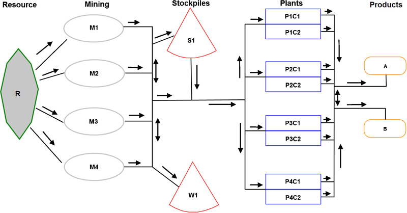
Example network of design options showing numerous flow paths
Examples of flow paths in Fig. 1 include the path from the resource (R) to mine 1 (M1) to stockpile 1 (S1) to plant 1 (P1) through circuit 1 (C1) to product A which would be RM1S1P1C1A, the path from the resource (R) to mine 1 (M1) to waste stockpile 1 (W1) which would be RM1W1, the path from the resource (R) to mine 1 (M1) to stockpile 1 (S1) to plant 4 (P4) through circuit 2 (C2) to product B (B) which would be RM1S1P4C2B and the path from the resource to mine 3 (M3) to stockpile 1 (S1) to plant 3 (P3) through circuit 1 (C1) to product A (A) which would be RM3S1P3C1A. This is only a small number of the potential paths through the network.
Stockpiling
Stockpiling is used in mine operations for many reasons including blending of material, storage of excess mine production, storage of waste material and storage of low grade ore for future production. When material is stockpiled, the grade and tonnage of the material is known. However, as the material is mixed on the stockpile, the grade and the tonnage become unknown. Since the quantity of material in the stockpile is unknown before the optimisation, this gives rise to a non-linear constraint. To solve this problem, virtual grade bins are created in the stockpile. These grade bins have a maximum and minimum grade of material which can enter the bin. As material is added to a stockpile, it will be fed into a grade bin that has a suitable grade range. Many grade bins can be created without adversely affecting the performance of the model which limits the averaging effect.
Stochastic parameters
The model incorporates uncertainty around the input parameters by MCS. Each simulation of values represents a ‘state of the world’ that is equally probable in the future. Various parameters can be incorporated in the model, for example price, capital cost, operating cost, equipment utilisation, recovery and time to build. Running a set of simulations is intended to give a representative sample of the future ‘states of the world’.
Models
Three different models have been proposed in order to justify increased flexibility to determine a flexible design, a robust design and an operational design. All models use MCS and MIP techniques to determine a system design. The fundamental difference between the models is that under a robust design, multiple ‘states of the world’ are considered together, while a flexible design considers just one ‘state of the world’ at a time. An operational design is developed by determining a fixed design for the first couple of periods and having a flexible design for periods after that. The flexible design model has been published previously in (Groeneveld et al., 2009; Groeneveld and Topal, 2011). The robust model is outlined in this paper and the operational plan is a new hybrid of these two models with the main difference that the design in the initial years is fixed. That is no binary value exits for design options in the initial periods.
Flexible design
Some researchers (Groeneveld et al., 2009; Groeneveld and Topal, 2011) have previously outlined a methodology for undertaking flexible mine design. The basis of these models was to optimise a design for a given single state of the world. This was achieved by including mining, plant and capacity constraint design options in the system and allowing the MIP model to internally handle the design options. MCS was used to generate these different ‘states of the world.’
This methodology assumes that a decision maker makes optimal decisions based on the knowledge of all states of the project over time (i.e. what price and costs occurred over time). In reality, forecasting the exact final state of a project is difficult if not impossible. The proposed methodology provides information and insight that can be used by the decision maker in conjunction with other tools to make timely, informed and value adding decisions.
Robust design
A new robust design methodology is proposed in this paper to develop a design that better handles all ‘states of the world’ as opposed to just a single design. It uses the same concepts and assumption developed in the flexible design model but differs by considering numerous states at once. A robust design is achieved by solving one ‘large’ MIP model that generates one design from multiple possible options. In essence, this design is the one which handles a range of conditions the best out of all possible options.
Operational design
An operational design methodology is proposed as a practical alternative to overcome the limitations of the robust and flexible methods. Essentially, an operational design is where the initial years of a fully flexible design have been fixed by the modeller. This allows management to make decisions today to enable the business to be an ‘ongoing’ concern. By not fixing future decisions, management can maintain flexibility in order to benefit from any upside potential and minimise any downside risk. As this method incorporates future flexibility into the analysis, the impact of the initial fixed decisions can be tested and tweaked in order to maximise value.
Robust model formulation
The developed MIP model optimises the system design for a risk neutral investor for all simulated ‘states of the world’. Each design option can impact capital commitment, revenue generated and operating expenses. The optimisation process seeks to determine the design with the highest equally weighted net present value for all given financial and technical scenarios. An outline of the mathematical formulation is provided below.
Notation
Indices
a grade bin of material within a parcel
product type
dependent options
flow path of material through the design network
grade element of material within a resource
bin of material within a stockpile: this bin will have a maximum and minimum grade of material which can enter
design options
mining options within the set of design options
simulated ‘state of the world’
parcel of material
required rate of return on the project
time period step (periods do not need to be equal)
stockpiling options within the set of design options
tolerance factor for the deviation of the mining of a bin within a parcel
Capitalised indices are the maximum value or upper limit of that index.
Parameters
the capital cost of option l in time t for trial n
the capacity of product d in time t for trial n
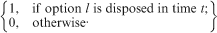
the disposal cost of option l in time t for trial n
the lag time between these relationships (i.e. build option two, three periods after option one)
the fixed cost saved from not operating option l from time t for trial n to the end of the project life T
the fixed cost of operating option l from time t for trial n to the end of the project life T
the lower grade limit of grade g product d
the lower grade limit of bin j
the upper grade limit of grade g product d
the upper grade limit of bin j
the grade of parcel p bin b
the grade g through plant l for trial n
the calculated average, maximum or minimum metal units of grade g in stockpile s in bin j
the capacity of option l in time t for trial n
the stockpile capacity of stockpile s in time t for trial n
the mining cost from parcel p to bin b through mine option l in time t for trial n
the sale price of grade element g for product d in time t for trial n (in $/metal unit)
the recovery of material through circuit l
the calculated average, maximum or minimum recovery for all material in stockpile s bin j
the available resource of parcel p bin b
the available resource of the successor parcel p+1
the variable cost of option l in time t for trial n
Variables
the metal units of grade g produced for product d in time t for trial n
the flow in from stockpile s bin j in time t for trial n
the flow out from stockpile s bin j in time t for trial n
the tonnage from parcel p bin b through flow path f in time t for trial n
the tonnage mined through flow path f in time t for trial n
the tonnage mined from parcel p bin b in time t for trial n
the tonnage mined from the successor parcel p+1 bin b in time t for trial n
the dependent option e of Yl,t
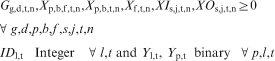
Formulation
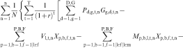
Objective function
The objective function seeks to maximise the equally weighted before tax net present value (NPV) for all simulated ‘states of the world’
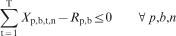
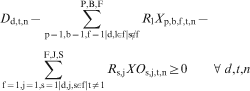
Resource constraints
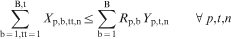
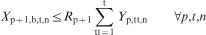
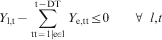
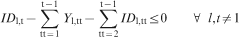
Option constraints
Stockpiling constraints
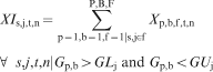
Product constraints
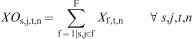
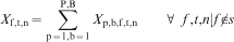
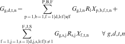
Flow balance constraints
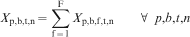
equation (18): the tonnage from a bin equals the tonnage through all paths from that bin
equation (19): the tonnage mined through each flow path that does not go through a stockpile equating to material mined from each parcel and bin through the flow path
equation (20): the total amount of metal units recovered to a product equates to the metal content through all direct feed to a plant plus any material treated after being stockpiled.
Non-negativity and integrality constraint
These constraints enforce non-negativity and integrality of the variables, as appropriate
Illustrative case study
This case study examines the use of several different mining capacity and plant capacity options for a deposit. The deposit was divided into four parcels generated by a single deterministic optimisation, such as Gemcom Whittle pit shells. While this may be considered to be removing the optimality from the model upfront, it was primarily used as a starting point for ‘shape’ generation. Refinement through an iterative process could easily be undertaken to improve optimality. Additionally, the purpose of this case study is to examine the execution of mining and plant options, which is not heavily reliant on schedule and/or sequence of extraction.
Table 1 provides a summary of the deposit used in this case study. The case study uses a single resource model; however, multiple stochastic models could be included. For the purposes of this case study, a physical constraint exists between parcels in a sequential order, i.e. parcel two cannot start before parcel one is finished.
Summary of deposit
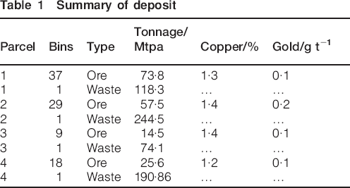
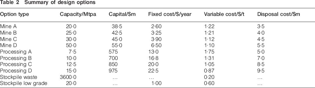
This case study will use four mining options, four processing options and two stockpiling options to undertake an analysis of the deposit. A summary of the options included in the model is outlined in Table 2. Stochastic variables for the following items incorporate the uncertainty into the model, commodity prices for gold and copper, capital cost, operating cost and plant utilisation. No detailed analysis of the underlying nature of the stochastic variables was undertaken, as detailed research in this area has been undertaken in other papers (Dowd and Xu, 1995; Godoy and Dimitrakopoulos, 2004; Dimitrakopoulos and Abdel Sabour, 2007; Topal, 2008; Shafiee and Topal, 2010).
Summary of design options
Distributions were set-up based on the parameters below. An assumption of constant growth in values was made and values were generated following the Markov property. For illustrating the techniques proposed, how the variables are simulated does not have a material impact. The distributions are:
gold price: starting value of $1200/oz, with a normal growth factor of 4% with standard deviation of 20%
copper price: starting value of $5000/t, with a normal growth factor of 5% with standard deviation of 10% and a correlation of 60% to the gold price
capital cost multiple: with a normal growth factor of 3% and a standard deviation 5% and a correlation to the gold price and copper price of 10%
operating cost multiple: with a normal growth factor of 4% and a standard deviation 10% and a correlation to the gold price and copper price of 30% and the capital cost index of 40%
plant utilisation: triangular distribution with a lower limit of 40%, midpoint of 85% and upper limit of 95%.
Four hundred simulations or ‘states of the world’ were used for the case study. Summaries of the ranges of values for gold and capital cost index are shown in Figs. 2 and 3 respectively.
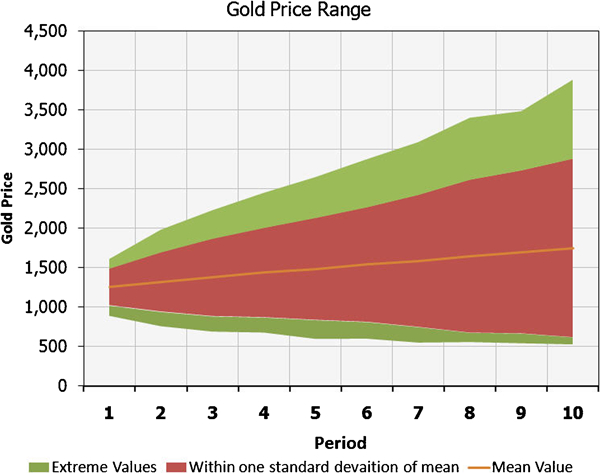
Gold price distribution over time
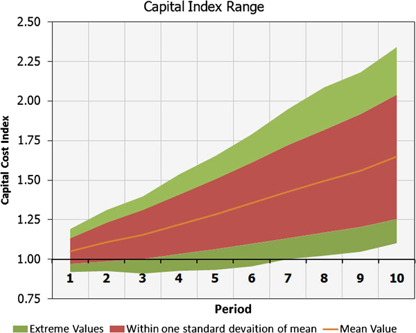
Capital cost index distribution over time
Results
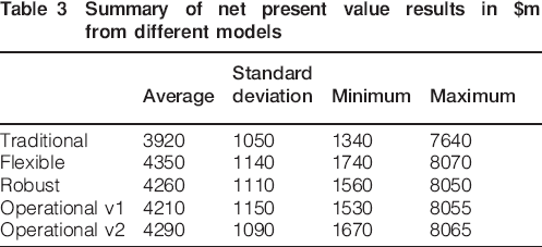
Five different design scenarios were modelled based on the three different design methodologies. A robust, a flexible and two operational designs, along with a traditional scenario were generated. All models were processed on a Quad core Ubuntu server with 2·66 GHz and 4 Gb RAM using the Gurboi 4·5·2 software. Solution times varied; however, for a fully flexible model, the average solution time was 30 s. A summary of the results is outlined in Table 3 with a discussion below.
Summary of net present value results in $m from different models
A traditional plan for operating a mine was generated by selecting the optimal design for a single deterministic scenario. The value for the stochastic parameters was generated by taking the starting values and applying the average growth factors only over time, i.e. no random variation was included. This produces a value which is similar to current industry practice for generating a design. For this scenario, the design generated was to build mine D, plant B and plant D in period one and mine A in period three with a net present value of $4050m. This design was then evaluated under the different simulated ‘states of the world’ to test its performance under uncertainty.
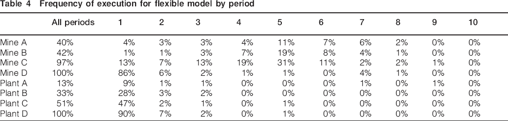
A flexible design model was used to produce an optimal design for each ‘state of the world’. This produced a result which provided an upper bound for the achievable value from the deposit, as the assumption is made that decision makers have perfect information and can therefore make perfect decision into the future. To analyse the options used in the model, a frequency of execution table and graph (Table 4 and Fig. 4 respectively) were generated. These show how often a particular option is used, calculated by dividing the number of times that an option is used by number of simulations. The available number of times that an option could be executed was 400. This showed that in every scenario, mine D and plant D were built. Mine C was built in most ‘states of the world’ and plant C was built in roughly half the ‘states of the world’. It also shows that around period five, there is increased need for mining capacity, as a handful of scenarios expand capacity in this period.
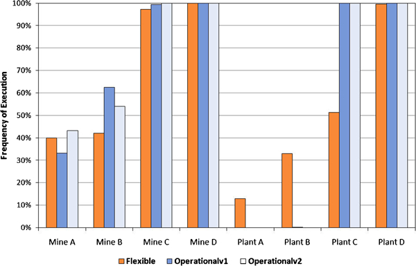
Frequency of execution graph for flexible and operational design scenarios
Frequency of execution for flexible model by period
Next, a robust design was generated by optimising the design for multiple ‘states of the world’ in one model. The resulting design was to build mine option D, plants C and D in period one and mine option C in period two. It should be noted that processing of the model with over 40 ‘states of the world’ is slow. This is because the number of linear variables doubles with each additional ‘state of the world’. For the model with 40 ‘states of the world’, there were 22 million variables. Gurobi 4·5·2. solves this model in 9 h on a Quad core 2·66 GHz Ubuntu Server with 4 GB of RAM. In order to test the sensitivity of the model, three scenarios were run with 25 ‘states of the- world’ and two scenarios with 30 ‘states of the world’. The states were all different scenarios generated from the MCS; however, the all generated the same design solution. So, arguably for this model, the number of ‘states of the world’ included was adequate at 25; however, this may be different for other models and should be tested for each deposit and set of options.
Based on the results of these results, two operational models were developed. The design was fixed for the first two periods. For period three onwards flexibility was available so the model could turn on and off design options. The model formulation for this was the same as the flexible model with the only difference being that the binary values for the design options were fixed in periods one and two. Two scenarios were constructed: version one involved mine D being built in period one, plant D in period one and plant C in period two and version two involved mine D in period one and mine C in period two, plant D in period one and plant C in period one. Version one of the design has less capacity in the initial years and produces less value than version two. Version two produces more value as it has greater capacity in the initial years (just having greater capacity earlier would not always produce greater value). Interestingly, version two design is exactly the same in the initial years as the design generated by the robust design. The difference is that the operational design allows for flexibility in the later years, thus the value of the operational design is higher than the robust design. Also, version one underperforms when compared with the robust design, so this would indicate to the modeller that there is a better operational solution to be found. However, had the robust design and the flexible design not established this base line, this finding would have been missed.
A value of risk graph is a cumulative probability distribution of project value in each ‘state of the world’. This is produced to highlight the differences between the models, as shown in Fig. 5. It allows a decision maker to quickly and easily compare the different design scenarios.
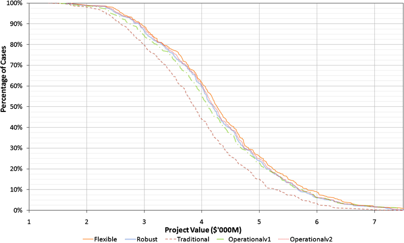
Value at risk graph for design scenarios
In comparing the models, it can be seen that the flexible model produces a higher expected value than any other model. This is as expected since the flexible model produces an optimal design for each ‘state of the world’. Such a flexible design may be impractical in reality. However, a robust design which does not incorporate any flexibility produces lower value than an operational and a flexible design as it is prohibited from reacting to change. The operational plan design has a lower expected value than the fully flexible design but higher than the robust design as it maintains flexibility in the later years and it is only the initial years that flexibility is limited. A traditional design produces the lowest expected value overall since it has no flexibility and is not optimised to handle uncertainties.
The differences between the expected values of each design approach can be attributed to two key aspects. First of all, actively managing the operation and allowing a flexible design (one that changes over time) will contribute significant additional value. The second component that contributes to additional value is being able to develop a robust fixed design which can handle a range of conditions. Refinement of the initial design chosen for the operational plan may lead to the discovery of plans with a higher expected value.
Conclusions
The paper has compared three different new design methodologies: flexible, robust and operational and extended the application of real options ‘in’ design theory to mining. It has been shown with clarity that all these methods outperform an approach which uses average values (the current traditional design approach). A fully flexible design approach generates the most value; however, it has practical implementation issues due to constant change. A robust design produces a single design that handles variation the best; however, the design does not change over time and therefore does not value active management. An operational design is proposed to overcome the limitations of the other design methodologies. While it does not produce as much value as the flexible design (which is only a theoretical maximum), it does produce more value than a robust design. Finally, the worst performing approach was the traditional approach which does not consider flexibility and uncertainty. Flexible operations produce greater project value than fixed, rigid operations, thus actively managing an operation is imperative to maximising value.