Absolute,relative and intrinsic rock brittleness at compression

Abstract

Many brittleness criteria have been proposed to characterise material behaviour under triaxial compression, but there is no consensus as to which criteria is the most suitable. It was shown recently that increasing σ₃ can lead to contradictory intact rock behaviour within different ranges of σ₃. For example, rock behaviour can be changed from class I (ductile) to class II (brittle) and then to class I again, based on the Wawersik and Fairhurst (1970) classification. Brittleness, in this case, can vary from absolute brittleness to absolute ductility. In this paper, it is argued that only two of the many existing criteria can properly describe the variation of brittleness within a wide range of confinements. These criteria rely upon energy balance and are based on sound physics principles.

Introduction

Brittleness is a very important mechanical property of intact rock, because it has a strong influence on the failure process and on the rock mass response to mining or tunnelling activities. However, the concept of brittleness in rock mechanics is yet to be precisely defined. Several brittleness criteria have been proposed to characterise material behaviour under compression (Baron et al., 1962; Walsh and Brace, 1964; Coates, 1966; Hucka and Das, 1974; Kidybinski, 1981; Batougina et al., 1983; Bergman and Still, 1983; Beron et al., 1983; Manjikov et al., 1983; Petoukhov and Linkov, 1983; Vardoulakis, 1984; Stavrogin and Protossenia, 1985; Recommendation, 1988; He et al., 1990; Andreev, 1995; Hajiabdolmajid et al., 2003; Tarasov, 2010, 2011; Tarasov and Randolph, 2011). Difficulties in reaching a consensus can be explained by the existence of two alternative failure mechanisms, tensile and shear fracturing, taking place under different compressive loading conditions. Also brittleness can be treated in two ways: as an intrinsic material property, or as the material behaviour under an external loading system contributing additional energy to the failure process.

Large seismic events are often produced when rock masses are submitted to triaxial compression generating violent shear failures. The correct determination of brittleness at such loading conditions is important to better understand these dynamic events. Unlike the generally accepted idea that rising confining pressure σ₃ makes rocks less brittle, the reality is more complex. Recently published papers (Tarasov, 2010, 2011; Tarasov and Randolph, 2011) showed that an increase in σ₃ can lead to contradictory rock behaviour within different ranges of σ₃. In fact, rock behaviour can be changed from class I (ductile) to class II (brittle) and then to class I again with brittleness variation from absolute brittleness to absolute ductility. In this paper, it will be shown that only two of the many existing criteria can properly describe the variation of brittleness within the whole range of testing conditions. These criteria rely upon energy balance and are based on sound physics principles.

Brief analysis of brittleness criteria

Rock brittleness is determined by different parameters obtained experimentally. These parameters can represent intrinsic material properties and also the loading conditions (e.g. the stiffness or elastic energy of the loading system). Brittleness indexes involving solely intrinsic parameters characterise the intrinsic material brittleness. Brittleness indexes based on ratios involving both intrinsic material parameters and loading system parameters, characterise material behaviour in relation to the loading conditions. For the purpose of this discussion these indexes are called relative material brittleness. The present paper focuses mainly on criteria characterising intrinsic rock brittleness.

Informative characteristics of intrinsic material properties, before and after the peak stress is reached, can be obtained from the complete stress–strain diagrams (see Fig. 1). A sketch of a rock specimen, with a potential shear fracture, loaded under triaxial compression is shown in Fig. 1a. The complete stress–strain curves through OABCD (Fig. 1b and c) illustrate two types of rock behaviour in the post-peak region: class I and class II according to the classification proposed by Wawersik and Fairhurst (1970). The graphs show the energy balance at three stages of deformation: at the peak stress (point B), at an intermediate post-peak stage (point R) and at the complete failure (point C). The hatched area OABE defined by the sloping lines represent the pre-peak rupture energy W_br spent to produce irreversible deformation ϵ_ir of the sample, before the peak stress is reached. The areas represented by white triangles delineated by the dotted lines correspond to elastic energy stored within the specimen body at the three mentioned stages of deformation. The area EBF corresponds to the elastic energy accumulated within the specimen material at the peak stress. The grey areas represent the post-peak rupture energy spent during the generation of the shear fracture.

Figure 1

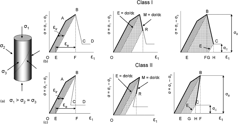
a schema of a specimen loading at triaxial compression; b energy balance at rock deformation in the case of class I behaviour; and c energy balance at rock deformation in the case of class II behaviour

The graphs illustrate the dynamics of transformation of the elastic energy accumulated within the specimen material at peak stress into the post-peak rupture energy. The white areas delineated by the dotted triangles (stored elastic energy) are replaced in the graphs by the grey areas (rupture energy). The stored elastic energy represents the source of the post-peak failure process and provides the physical basis for the post-peak failure regime. For class II, the shear fracture development occurs entirely due to the elastic energy available from the material. The failure process has a self-sustaining character with the release of excess energy corresponding to area HCBF (note that the small white dotted triangle GCH represents the unconsumed portion of the stored elastic energy after failure). The release of the excess energy can be transformed into the failure process dynamics, i.e. kinetic energy of flying fragments, seismic energy, fragmentation, heat, etc. For class I, the elastic energy available from the material is entirely consumed by the rupture process, and some additional amount of energy (area FBCG) is required to support this process.

Brittleness indexes based upon the ratio between the elastic energy and the post-peak rupture energy (or released energy) can be used to characterise the capability of the rock for self-sustaining failure due to the elastic energy available from the material. Such brittleness indexes actually characterise the degree of intrinsic instability of the material at failure. The graphs in Fig. 1 can therefore be used to determine brittleness from energy parameters. For a simplified estimation of the elastic energy dW_e withdrawn from the material specimen during the post-peak failure process between points B and C, it is assumed that the elastic modulus E = dσ/dϵ is the same at both points. It should be noted that the modulus E represents the unloading elastic modulus. (1) The graphs show that the post-peak rupture energy dW_r (grey area) is determined by the amount of withdrawn elastic energy dW_e plus the additional energy corresponding to area FBCG in the case of class I behaviour, or minus the excess released elastic energy corresponding to area HCBF in the case of class II behaviour. The excess (or released) energy is described by equation (2) (2) Here, M = dσ/dϵ is the post-peak modulus. M is negative for class I and positive for class II behaviour.

The post-peak rupture energy dW_r is described by equation (3). The equation takes into account the sign of post-peak modulus M for class I and class II behaviour (3) The brittleness index K₁ below is determined by the ratio between the post-peak rupture energy and the withdrawn elastic energy (Tarasov, 2010, 2011; Tarasov and Randolph, 2011) (4) The brittleness index K₂ represents the ratio between the excess (released) and the withdrawn elastic energy (Tarasov, 2010, 2011; Tarasov and Randolph, 2011) (5) It is known that the unloading elastic modulus E and the post-peak modulus M can vary significantly with the fracture development. However, two infinitely near points located on a post-peak curve (for example points B and C in Fig. 2) can be characterised by the same value of E. The corresponding modulus M is determined on the basis of a tangent line. Increments of withdrawn elastic energy dW_e, post-peak rupture energy dW_r and excess (released) energy dW_a associated with fracture development between the neighbouring points B and C are described precisely by equations (1)–(3). Using equations (4) and (5), brittleness indexes K₁ and K₂ can be determined for any stage of the post-peak process.

Figure 2

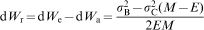
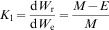
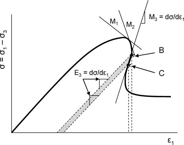
Illustration of local brittleness estimation by brittleness indexes K₁ and K₂

Brittleness indexes K₁ and K₂ characterise unambiguously the rock brittleness at different loading conditions. Figure 3 shows scales of rock brittleness indexes K₁ and K₂ with brittleness increasing from left to right (Tarasov, 2010, 2011; Tarasov and Randolph, 2011). The complete curves (differential stress σ versus axial strain ϵ₁) illustrate how the different curve shapes describe a variation in brittleness. It is assumed, for simplicity, that the pre-peak parts of the curves are the same. Areas defined by the large dotted triangles correspond to elastic energy W_e stored within the rock material at the peak stress, while the smaller white triangles on the right side of the curves represent the unconsumed portion of the stored elastic energy, within the material, after failure. The post-peak parts of the curves, which are characterised by the post-peak modulus M, are different for each curve. The grey areas represent the post-peak rupture energy dW_r associated with strength degradation at failure from the peak stress to the residual strength (horizontal part of the post-peak curves).

Figure 3

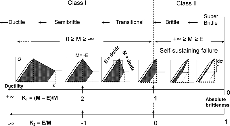
Scale of brittleness indexes K₁ and K₂ with characteristic shapes of complete stress–strain curves (Tarasov, 2010, 2011; Tarasov and Randolph, 2011)

Figure 3 shows variation in brittleness from absolute brittleness to ductility if read from right to left. The absolute brittleness has the following characteristics and parameters:

•.

The post-peak modulus is the same as the elastic modulus M = E.

•.

There is no portion of the stored energy transformed into post-peak rupture energy dW_r = 0.

•.

The withdrawn elastic energy is entirely transformed into excess energy dW_e = dW_a.

•.

K₁ = 0.

•.

K₂ = 1.

Within the range of brittleness indexes 1>K₁>0 and 0<K₂<1 the elastic energy dW_e withdrawn from the specimen material during stress degradation on the value dσ exceeds the corresponding rupture energy dW_r, leading to self-sustaining failure (brittle class II behaviour). The self-sustaining failure normally has a spontaneous character even for a hypothetically perfectly stiff testing machine. The greater the difference between dW_e and dW_r, the closer the material behaviour is to absolute brittleness and the more violent is the self-sustaining failure. It should be noted that the use of very stiff and servo-controlled loading machines allow in many cases controllable failure for rocks characterised by the positive post-peak modulus M due to the extraction of the excess elastic energy from the material body. For the range of brittleness indexes +∞>K₁ >1 and −∞<K₂<0 the rupture development is not self-sustaining (class I behaviour). Variation in failure regimes corresponding to an increase in the rock brittleness is indicated in the upper part of Fig. 4. These regimes are: ductile, semi-brittle, transitional, brittle and super-brittle. The characteristic features of the super-brittle regime are further discussed.

Figure 4

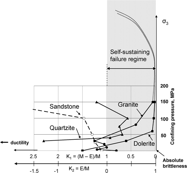
Variation of brittleness indexes K₁ and K₂ versus confining pressure σ₃ for rocks of different hardness (modified from Tarasov, 2010, 2011; Tarasov and Randolph, 2011)

Figure 4 shows the variation of brittleness index K₁ and K₂ for four rocks exhibiting different responses to rising confining pressure σ₃ (Tarasov, 2010, 2011; Tarasov and Randolph, 2011). The self-sustaining failure regime corresponds to 1>K₁>0 and 0<K₂<1. The sandstone curve indicates that an increase in confinement σ₃ makes the rock less brittle. This behaviour is typical for softer rocks. For the quartzite, increase in confinement σ₃ within the range of 0–100 MPa makes the material more brittle. At greater confinement the brittleness decreases. For the granite, increase in σ₃ within the range of 0–30 MPa makes it less brittle. When σ₃>30 MPa, the brittleness increases dramatically. The dolerite curve also shows very severe rock embrittlement. At σ₃ = 75 MPa, according to the brittleness index K₁, the dolerite became 250 times more brittle when compared to uniaxial compression (K₁(0) = 1·5; K₁(75) = 0·006). At σ₃ = 100 and 150 MPa, the brittleness increased significantly, further approaching absolute brittleness. The dotted lines indicate the expected brittleness variation for granite and dolerite at greater values of σ₃: the brittleness continues to increase until it reaches a maximum at some level of σ₃ and then decreases, as all rocks become ductile at very high confining stresses. It is estimated (Tarasov, 2010, 2011; Tarasov and Randolph, 2011) that the maximum brittleness for granite is reached at σ₃≈300 MPa. For rocks that are as hard as quartzite, the mode of brittleness variation is similar, but the maximum brittleness is lower and the range of confining pressure where embrittlement takes place is smaller.

Brittleness indexes similar to K₁ and K₂ were proposed earlier in (Batougina et al., 1983; Bergman and Still, 1983; Manjikov et al., 1983; Petoukhov and Linkov, 1983; Stavrogin and Protossenia, 1985) (6) (7) However, the brittleness indexes k₃ and k₄ include some uncertainties which can lead to conflicting results for estimating the brittleness at different loading conditions. Also these indexes do not allow the creation of continuous and unambiguous scale of brittleness similar to the one presented in Figs. 3 and 4. Scales of brittleness for k₃ and k₄ are stretched between k = −∞ and k = +∞, and the extreme points of each scale (−∞ and +∞) are characterised by the same shape of stress–strain curves. Other zones of discontinuity are located in a central part of the scales between conditions of the absolute brittleness (k₃ = 0·5 and k₄ = 1) and absolute ductility (k₃ = 0 and k₄ = 0). Hence, the brittleness indexes k₃ and k₄ are not ideal for brittleness characterisation at different levels of confining pressure.

Brittleness indexes representing ratios of different combination between pre-peak and post-peak strain (k₅ and k₆, equations (8) and (9)) were discussed in other publications (Andreev, 1995; Recommendation, 1988; He et al., 1990). Note that ϵ_e is the elastic strain, ϵ_p is the post-peak strain and ϵ_tp is the total irreversible post-peak strain (8) (9) It is found that these strain based indexes also give ambiguous results when used to characterise the brittleness. For example, three stress–strain curves in Fig. 5 have the same elastic modulus E. At some stages of post-peak deformation, they have a very different post-peak modulus M, which suggests very different brittleness. However, brittleness indexes k₅ and k₆ based on ratios between values of elastic and post-peak deformations determined at a stage shown in Fig. 5 have the same value for all three rocks.

Figure 5

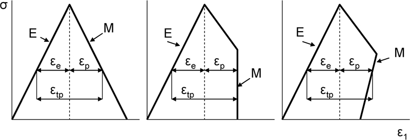
Schema for estimation of rock brittleness from elastic and post-peak deformations

Brittleness indexes based on different combinations of other parameters may give conflicting results at different loading conditions, because unlike K₁ and K₂, they do not have any physical foundation. A number of examples are discussed below.

Brittleness indexes involving parameters associated with the pre-peak irreversible deformation (k₇, k₈ and k₉) have also been proposed (Baron et al., 1962; Coates, 1966; Hucka and Das, 1974; Kidybinski, 1981). (10) (11) (12) However, experimental studies have shown that the value of the pre-peak irreversible deformation ϵ_ir and the corresponding energy W_br (see Fig. 1) do not correlate with post-peak rock properties. The graphs in Fig. 1 show that the same pre-peak irreversible behaviour can be followed by both class I and class II behaviour in the post-peak region. Furthermore, increase in confinement (σ₃) causing increase in pre-peak ductility can lead to both an increase or decrease in post-peak ductility.

The determination of intrinsic material brittleness from compressive R_c and tensile R_t strengths indexes, e.g. k₁₀ = R_c/R_t (Walsh and Brace, 1964; Beron et al., 1983; Vardoulakis, 1984) gives conflicting results when samples are tested under triaxial compression. It is accepted that the difference between R_c and R_t increases with an increase in brittleness. However, at greater confinement (σ₃), despite the fact that the compressive strength R_c increases the material behaviour can be accompanied by both increase and decrease in material brittleness as shown in Fig. 4. Determination of brittleness k₁₁ from Mohr's Envelope (Hucka and Das, 1974) implies the decrease in brittleness with rising confining pressure σ₃ and cannot reflect rock embrittlement within a certain range of high confining stress (σ₃).

Failure mechanisms providing high (class I) and low (class II) rupture energy

Figure 6a shows four stages of shear rupture development in a specimen when submitted to triaxial compression. A load cell and an axial gauge mounted on the specimen are used to measure the average load bearing capacity and the strain of the specimen during the post-peak stage of the loading procedure. The real shear resistance and displacement along the future failure plane are very non-uniform. Three specific zones can be distinguished (see Fig. 6a-ii):

Figure 6

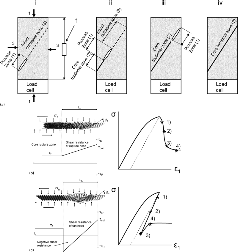
a four stages of shear rupture development in a specimen at triaxial compression; b frictional and c frictionless concepts of shear fracture development

the process zone (or rupture head) where the failure process is in progress

ii.

the core frictional zone located behind the head where the full friction is mobilised

iii.

the intact zone in front of the head where the resistance is determined by the cohesive strength.

With fracture propagation the cohesive strength of decreasing zone (iii) is substituted by the frictional resistance of increasing zone (ii). This process is accompanied by the decrease in bearing capacity of the specimen from the cohesive strength to the frictional (residual) strength. The fracture mechanism operating within the head (process) zone (i) plays the key role in the character of transformation from the cohesive to frictional strength.

It is known that a shear rupture can propagate in its own plane due to the creation of short tensile cracks in front of the rupture tips (Cox and Scholz, 1988; Reches and Lockner, 1994; Reches, 1999). This forms the universal structure of shear ruptures represented by an echelon of blocks (or slabs) separated by tensile cracks – known as ‘book-shelf’ structure (Peng and Johnson, 1972; Cox and Scholz, 1988; King and Sammis, 1992; Reches and Lockner, 1994; Reches, 1999;) or Ortlepp shears (van Aswegen, 2008; Ortlepp, 1997). The initial angle β₀ of the tensile crack and block inclination to the shear rupture plane is about 30–40° (Horii and Nemat-Nasser, 1985). Shear displacement along the fault causes rotation of the blocks of the ‘book-shelf’ structure between the rupture surfaces (Peng and Johnson, 1972; Cox and Scholz, 1988; King and Sammis, 1992; Reches and Lockner, 1994; Tarasov, 2010, 2011; Tarasov and Randolph, 2011).

Figure 6b illustrates the essence of the shear rupture mechanism providing large rupture energy. Blocks located in the front part of the head create significant resistance to shear; however, they collapse with rotation providing gradual transformation of shear resistance within the head zone from cohesive to frictional levels. A graph under the shear rupture in Fig. 6b shows the shear resistance variation along the fault head. The crushing and comminution of blocks within the head zone can absorb large amounts of energy. This is expected since the development of shear fractures requires displacement to occur along the total fault. This form of rupture development is classified as a crack-like mode. Such a rupture mechanism normally produces a class I material behaviour in the post-peak region. Four points on the stress–strain curve on the right correspond to the four stages of deformation shown in Fig. 6a.

Figure 6c illustrates a model where rotating blocks can withstand the rotation without collapse by behaving as hinges (see details in Tarasov, 2010, 2011; Tarasov and Randolph, 2011). Owing to consecutive formation and rotation of the blocks, these should form a fan structure within the rupture head. A remarkable feature of the rotating blocks (hinges) in the second half of the fan structure (where β>90°) is the creation of active forces under the effect of normal stress applied. A graph under the shear rupture in Fig. 6c shows the shear resistance variation along the fault head. The bottom part of the graph represents active forces (negative resistance) acting in the second half of the head and assisting the fault displacement. In the core zone represented by blocks that have completed their rotation the normal residual friction is restored.

The fan structure represents a self-equilibrating mechanism and can move spontaneously as a wave with very small shear resistance. In the idealised fan-head model, the resistance to rupture propagation is determined only by the tensile strength of the material associated with consecutive formation of blocks in front of the propagating rupture. It is important that the fan-head can propagate independently of the core zone, which can remain immobile due to high frictional resistance. Hence, this mechanism creates conditions for a pulse-like mode of fracture propagation. In this situation the rupture energy is determined by shear resistance of the fan head only. The fan-head rupture mechanism represents the most energy efficient shear rupture mechanism.

This mechanism is responsible for class II behaviour with extremely small rupture energy approaching absolute brittleness. The stress–strain curve in Fig. 6c shows that at stage 3 of the fracture propagation, the bearing capacity of the specimen can be less than at stage 4. It is because the shear resistance of the head (process) zone can be close to zero, decreasing the bearing capacity of the specimen. The longer the relative rupture head (process zone (i)) is, the smaller the shear resistance at stage 3 of the rupture propagation. The full frictional resistance is mobilised at stage 4 after the head completely propagates through the specimen.

The examples discussed show that shear rupture mechanisms involving the book-shelf structure can be responsible for the delay in friction mobilisation at failure. A concept of strain dependent mobilisation of strength at failure on the basis of other failure mechanisms is discussed in Hajiabdolmajid et al., 2003. A special strain dependent brittleness index k₁₂ was introduced to consider the contribution of the cohesive and frictional strength components during the failure process. From the physical point of view the brittleness index k₁₂ reflects the presence of both tensile and shear mechanisms in inducing microcracks. This concept, however, implies an increase in ductility with rising confining pressure. Therefore, this cannot explain the very severe embrittlement observed in hard rocks under increasing confinement (σ₃) and the extremely low rupture energy at high levels of σ₃ (see Fig. 4). The reasons for rock embrittlement due to rising σ₃ are discussed in (Tarasov, 2010, 2011; Tarasov and Randolph, 2011) where the brittleness indexes K₁ and K₂ were first introduced.

Natural shear fractures can be at different stages of their development. Their shear resistance and brittleness at the post-peak failure stage can correspond symbolically to different points on the stress–strain curves shown in Fig. 6b and c. The brittleness (degree of instability) and energy release during the rupture development depends on the failure stage and the rupture mechanism. The discussed brittleness indexes K₁ and K₂ can be used for characterisation of the stability conditions.

We should note that the proposed criteria K₁ and K₂ can be used for the relative stability characterisation at uniaxial compression also. In this situation, despite the fact that the failure process is associated with the development of large tensile cracks, the stability of the loading process in the post-peak region is determined by the total rupture energy and the available elastic energy characterised by the complete stress–strain curves.

Relative rock brittleness and applications

Figure 7a shows two generic load–displacement curves for two different rocks obtained on specimens of the same dimensions. These two rocks have the same brittleness index K₁ and K₂, because they are characterised by the same ratio between the elastic and post-peak modules: E′₁/M′₁ = E′₂/M′₂. However, the behaviour of these rocks during testing on the same loading system can be very different. The dotted lines on the graph characterise the stiffness L of the loading system. For rock number 1, L<M′₁ and in accordance with Cook (1965), failure should be unstable while for rock number 2, L>M′₂ and failure should be stable. On the basis of equation (13) (Cook, 1965), the brittleness of these two rocks can be determined in relation to the loading system. Referring to the discussion in the section on ‘Brief analysis of brittleness criteria’, such classification of brittleness reflects the relative brittleness of rocks instead of the intrinsic material brittleness. (13) The use of intrinsic or relative brittleness for estimation of degree of instability in practice depends on loading conditions. For instance, rock mass surrounding an extended underground excavation represents a loading system with respect to pillars supporting the excavation (see Fig. 7b). In this case, the degree of total instability of this construction can be characterised by index k_R representing relative brittleness. In the case of shear fracture propagation within intact rock mass (Fig. 7c), the use of intrinsic brittleness indexes K₁ and K₂ are more appropriate.

Figure 7

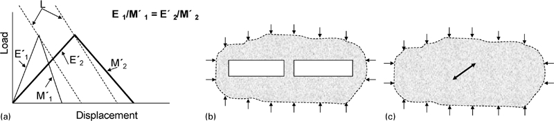
a load–displacement curves for two rocks having the same intrinsic and different relative brittleness, b rock mass involving an underground excavation with a pillar and c rock mass involving a shear fracture

Conclusions

The applicability of various criteria for assessing rock brittleness under triaxial compression has been analysed. It is shown that only two of many existing criteria can properly describe the intrinsic material brittleness within the whole range of brittleness variation from the absolute brittleness to ductility. These criteria are based upon the balance between elastic energy accumulated within the material specimen and two forms of post-peak energy associated with the failure process: the rupture energy and the excess (released) energy. The brittleness indexes based on the ratio between these parameters allow for the representation of the two classes of rock behaviour (class I and class II) in the form of continuous, monotonic and unambiguous scale of brittleness. Other existing criteria do not provide unambiguous characterisation of rock brittleness at different loading conditions under triaxial compression.

Footnotes

Acknowledgements

This work has been supported by the Centre for Offshore Foundation Systems (COFS) at The University of Western Australia, which was established under the Australian Research Council's Special Research Centre scheme and is now supported by the State Government of Western Australia through the Centre of Excellence in Science and Innovation program. This support is gratefully acknowledged.

This paper has been reproduced with the kind permission of the Australian Centre for Geomechanics, The University of Western Australia. The Sixth International Seminar on Deep and High Stress Mining proceedings volume, 28–30 March 2012, Perth, Australia (ISBN 978-0-9806154-8-7, ).

This paper is part of a special issue on Deep and High Stress Mining

References

Andreev

. 1995. Brittle failure of rock materials, Rotterdam, Balkema.

Baron

, Loguntsov

, Posin

. 1962. Determination of rock properties, Moscow, NTILGD.

Batougina

, Petoukhov

, Vinokur

, Smirnov

, Rabota

. 1983. Methodological instructions for rockburst prophylaxis accounting the deposit geodynamics, Leningrad, VNIMI.

Bergman

SGA

, Still

1983. Rockburst problems in a 2·6 million m³ underground crude oil storage in granite, Proc. 5th Cong. ISRM, April 1983, Melbourne, Australia, ISRM, D302–D309.

Beron

, Vatolin

, Koifman

, Mohnachev

, Chirkov

. 1983. Rock properties under different loading regimes, Moscow, Nedra.

Coates

. 1966. Experimental criteria for classification of rock substances, Int. J. Rock Mech. Min. Sci., 3, 181–189.

Cook

NGW

. 1965. The failure of rock, Int. J. Rock Mech. Min. Sci., 2, 389–403.

Cox

SJD

, Scholz

. 1988. On the formation and growth of faults: an experimental study, J. Struct. Geol., 10, 413–430.

Hajiabdolmajid

, Kaiser

, Martin

. 2003. Mobilised strength components in brittle failure of rock, Geotechnique, 53, (3), 327–336.

10.

, Okubo

, Nishimatsu

1990. A study on the class II behaviour of rock, Rock Mech. Rock Eng., 23, 261–273.

11.

Horii

, Nemat-Nasser

1985. Compression-induced microcrack growth in brittle solids: Axial splitting and shear failure, J. Geophys. Res., 90, 3105–3125.

12.

Hucka

, Das

1974. Brittleness determination of rocks by different methods, Int. J. Rock Mech. Min. Sci., 11, 389–392.

13.

Kidybinski

1981. Bursting liability indexes of coal, Int. J. Rock Mech. Min. Sci., 18, 295–304.

14.

King

GCP

, Sammis

. 1992. The mechanisms of finite brittle strain, PAGEOPH, 138, (4), 611–640.

15.

Manjikov

, Mansourov

, Pougacheva

, Tileguenov

. 1983. Laboratory estimation of rockbursting danger, SSDRRMODMA, Frounze, Ilim, 106–116.

16.

Ortlepp

. 1997. Rock fracture and rockbursts. Johannesburg, SAIMM.

17.

Peng

, Johnson

. 1972. Crack growth and faulting in cylindrical specimens of Chelmsford granite, Int. J. Rock Mech. Min. Sci., 9, 37–86.

18.

Petoukhov

I.M.

, Linkov

A.M.

(1983. Mechanics of rockburst and outburst, Moscow, Nedra

19.

Reches

1999. Mechanisms of slip nucleation during earthquakes, EPSL, 170, 475–486.

20.

Reches

, Lockner

. 1994. Nucleation and growth of faults in brittle rocks, J. Geophys. Res., 99, (B9), 18159–18173.

21.

Recommendation . 1998. Recommendation for determining the total Mohr strength envelope and deformability for rock Leningrad, VNIMI.

22.

Stavrogin

, Protossenia

. 1985. Rock strength and excavation stability in great depth, Moscow, Nedra.

23.

Tarasov

. 2010. Superbrittleness of rocks at high confining pressure, Proc. 5th Int. Semin. on Deep and High Stress Mining (Deep Mining 2010), (ed. , van Sint Jan

, Potvin

), October 2010, Santiago, Chile, Australian Centre for Geomechanics, 119–133.

24.

Tarasov

. 2011. Universal scale of brittleness for rocks failed at compression, Proc. 13th Int. Conf. of the International Association for Computer Methods and Advances in Geomechanics, August 2011, Melbourne, Australia, International Association for Computer Methods and Advances in Geomechanics, 669–673.

25.

Tarasov

, Randolph

. 2011. Superbrittleness of rocks and earthquake activity, Int. J. Rock Mech. Min. Sci., 48, 888–898.

26.

van Aswegen

2008Ortlepp shears – dynamic brittle shears of South African Gold Mines, Proc 1st Southern Hemisphere International Rock Mechanics Symp. (SHIRMS)(, Potvin

, ), Vol. 2, Fundamental and Petroleum, September 2009, Perth, Australia, Australian Centre for Geomechanics, 111–119.

27.

Vardoulakis

1984. Rock bursting as a surface instability phenomenon, Int. J. Rock Mech. Min. Sci., 21, 137–144.

28.

Walsh

, Brace

. 1964. A fracture criterion for brittle anisotropic rock, J. Geophys. Res., 69, 3449–3456.

29.

Wawersik

, Fairhurst

1970. A study of brittle rock fracture in laboratory compression experiments, Int. J. Rock Mech. Min. Sci., 7, 561–575.