Optimisation of a stochastic rock fracture model using Markov Chain Monte Carlo simulation

Introduction

Australia is a world leader in the development of economically viable production of geothermal energy from hot dry rock (HDR) with key projects including Geodynamics’ Cooper Basin project near Innamincka, South Australia. The heat resource is a result of decaying radioactive elements. Geoscience Australia estimates that by exploiting just 1% of the geothermal heat resource within the uppermost 5 kms of the Earth's crust could provide 26 000 times our annual energy consumption (GA, 2011). There are, however, still many complex unresolved issues in HDR geothermal energy production; one of the most critical is the creation of an effective heat exchange fracture network inside the reservoir to create an enhanced geothermal system (EGS) with the capability to produce flowrates in excess of 100 l s⁻¹ to sustain efficient heat exchange between the fluid and the in situ rock to guarantee sufficiently high temperatures of the extracted fluid and the sustainability of the reservoir. Potential HDR geothermal systems occur in deep underground crystalline rock. The rock matrix (granite) is almost impermeable and the only viable pathway for geothermal flow is through a fracture network. Natural fractures in HDR are generally closed or sealed with very low hydraulic conductivity (with micrometre scale hydraulic apertures). The creation of a viable geothermal reservoir, appropriate for industrial scale exploitation, is usually achieved by hydraulically stimulating fractures to create the EGS. After the fracture stimulation, it is critical to understand the fracture system within the reservoir as that will provide the basis for the modelling of flow within, and heat extraction from the EGS so that the design and performance assessment of the entire energy production system can be performed.

However, the characterisation of such a fracture network is a very difficult problem as the whole fracture system is not observable on any meaningful scale and the only reference data related to the fracture system are either from geophysical borehole logs and/or sparse seismic events kilometres beneath the surface and detected during hydraulic stimulation. For these reasons current models of fracture systems used for HDR flow modelling are oversimplified representations of reality. They either use an equivalent porous media approach, single fracture representation or a combination of both.

As direct measurement/observation of the fracture system is not possible the only way to construct the fracture model for the reservoir is via a stochastic process. Stochastic fracture modelling is the general approach in which locations, size, orientation and other properties of fractures are treated as random variables with inferred probability distributions. In the simplest case, once the parameters of the distributions are inferred, the rock fracture model is constructed by Monte Carlo simulation (Xu and Dowd, 2010). First, the fracture locations are generated, usually by a Poisson distribution in which fracture intensity for a particular area is either assumed to be constant or is derived from geostatistical estimation or simulation. Second, the orientation of each fracture is generated, most commonly from a Fisher distribution. Finally, the size of each fracture is generated from a specified distribution, the most common being exponential, lognormal or gamma. Other fracture properties, such as aperture width and fracture strength, can then be added to the network by additional Monte Carlo steps. Options for fracture intersections and fracture termination can also be incorporated. Simulated fracture models are usually validated by sampling the model (using scan lines or areas on cross-sections) and assessing the extent to which the sampled values conform to the statistical models derived directly from survey data (Kulatilake et al., 2003). In HDR EGS, however, this validation approach is of very limited value as only downhole surveys are possible and these can only reveal very limited information about the fracture density and orientation near the wellbores.

Fracture stimulation causes planes of existing (naturally occurring) fractures to slip against each other due to the reduction in effective normal stress. Slipping causes misalignment of fracture surface profiles causing lateral dilation, which essentially causes the hydraulic aperture of the fracture to increase (Baisch et al., 2009). In addition, fracture stimulation causes the existing fractures to propagate and creates new fractures. The final product of stimulation is a fractured rock mass that can be exploited to produce heat by using injection and production wells intersecting the reservoir. During fracture stimulation, fracture initiation, propagation and slipping generate microseismic events that can be monitored and their spatial locations determined. The resulting seismic point cloud can be used to determine not just the geographical extent of the HDR reservoir and the amount of fracturing but also the fracture network within the reservoir (Xu et al., 2011). Establishing the fracture network reservoir model conditioned by this seismic point cloud is critical in creating a more realistic and reliable fracture model for the HDR EGS.

Data conditioning in two-dimensional fracture modelling is widely reported in the literature but publications for conditioning three-dimensional fracture networks are very limited due to the complexity involved. Mardia et al. (2007) described an attempt to condition a fracture model by borehole intersection data using Markov Chain Monte Carlo (MCMC) simulation. We describe, in this paper, the extension of this method to use only the seismic event point cloud to condition fracture models constructed for Geodynamics’ HDR reservoir in the Habanero well field.

Markov Chain Monte Carlo method

There are two major mechanisms of fracturing during HDR fracture stimulation. The first is fracture planes of existing fractures slipping against each other due to the reduction of the effective normal stress acting on the fracture planes, which, in turn, may cause the fracture to propagate. The second is the initiation of new fractures due to hydraulic pressure exceeding the strength of the rock. In either case, it is reasonable to assume that seismicity caused by either the fracture slipping/propagation or fracture initiation occurs only on the fracture plane. In other words, an accurately conditioned fracture model should intersect these points.

In reality, fracture planes are highly tortuous. It is impossible to represent all fractures by tortuous surfaces using a reasonable number of parameters and some simplification is required. Common approaches include circular discs, elliptical discs, planar polygons or planes with infinite extents. The validity of this representation is based on the assumption that fracture planes in the fitted model will follow closely the actual tortuous surfaces of the fractures in the reservoir, or in other words, the fitted fracture model is the first order approximation of reality. Within this framework, even the best fitted model will not intersect all seismic points but the distance of the points to fracture planes can be used as a criterion to assess the goodness-of-fit of the fracture model. It should be noted that the accuracy of the seismicity detection and the inversion process in deriving the locations of seismic points are not topics of this paper. Readers interested in these topics should consult Baisch et al. (2006).

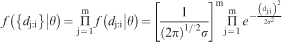
Assume there are m conditioning seismic events and n fractures in the fracture model. A projection distance for each seismic event j (j = 1,…,m) as d_j:i defined as the distance of point j to fracture plane i which is the shortest distance from point j to all fracture planes is introduced. Point j is then said to be associated with and only with fracture plane i. Because of the first order approximation of the fracture model, the complete set of projection distances d = {d_j:i}∀j will exhibit random variation from the fitted fracture planes. A Gaussian model is the most appropriate statistical model to describe random variation, or noise, from a first order approximation, i.e., , where σ² measures the degree of tortuous variability of fracture surfaces. The likelihood for the set of seismic event points P = {P_j} given a set of fitted fractures F = {F_i} can then be defined as 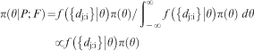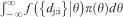(1) with the set of parameters θ = [(x_i, y_i, z_i, α_i, β_i, γ_i, a_i, b_i), i = 1,2…n], where (xⁱ, yⁱ, z_i) are coordinates of the centre of fracture plane i, (a_i, b_i) are the major and the minor axes of the ellipse containing the fracture polygon, (α_i, β_i) are dip direction and dip angle of the fracture plane and γ_i is the rotation angle of the major axis of the ellipse against the dip direction of the fracture plane. The posterior distribution given P and F is then (2) and π(θ) is the prior distribution or prior belief for the parameters of the set of fractures F. Note the normalising constant does not usually need to be calculated as the parameters of the posterior distribution π(θ|P; F) can be derived from the numerator.

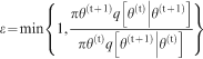
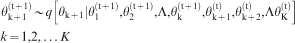
In practice, the number of fractures could be in the order of millions and the dimension of θ will be the same order of magnitude. The posterior distribution of θ is therefore analytically intractable. One way to derive samples of the parameters θ from the posterior distribution π(θ|P; F) is to construct a Markov chain using MCMC. A Markov chain is generated by Monte Carlo sampling of a proposal distribution, also termed transition kernel q, as follows (3) and the move of the chain to θ^(t+1) is accepted with probability equal to the so called Hastings ratio (4) A symmetric transitional kernel is the most commonly used and that is the basis of the Metropolis–Hastings algorithm. For high dimensions of θ, a Gibbs sampler is more effective and will be used in our implementation. In this process, the sampling is from the full conditional distributions taking into account the current states of the parameters, i.e. (5) The Markov transition from θ^(t) to θ^(t+1) is done in K steps where K is the total number of parameters in θ; t is the time step. If the generated Markov chain is long enough, the samples, in theory, should converge to the stationary distribution. A burn-in period is necessary for the chain to reach its stationary stage after which samples for each parameter can then be summarized to derive the parameter estimate (expected value, according to the law of large numbers).

Mardia et al. (2007) described a detailed MCMC implementation for fracture fitting given a set of fracture borehole intersection points. More general descriptions of MCMC can be found in Gamerman (2006).

Application in fracture modelling of Habanero Reservoir

The Habanero wells are the key components of Geodynamics’ HDR geothermal project in the Cooper Basin, South Australia. These wells have been drilled to depths of ∼4400 m below the surface or ∼700 m into the bedrock where temperatures reach 250°C (Baisch et al. (2006)). A large scale hydraulic fracture stimulation was conducted at Habanero 1 between November 6 and December 22, 2003 (Weidler, 2005). The seismic events were recorded and later processed to derive their locations. The data set used in this study is the Q-Con dataset which contains a total of 23 232 seismic events covering an approximate area of 2·5 km² (Baisch et al. (2006)). The absolute hypocentre locations of these events are shown in Fig. 1, in which the locations of Habanero 1 and 3 wells are also shown. The seismic point cloud clearly indicated an ideal subhorizontal reservoir formed by the stimulation process which is gently dipping in the Southwest direction.

OPEN IN VIEWER

Figure 1

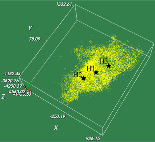
Absolute hypocentre locations of seismic events

We start with fitting only one fracture for the reservoir to test the effectiveness of the MCMC algorithm. In this case θ has a dimension of 8, i.e. Using σ² = 50 and 2000 as the burn-in period, after 16 000 iterations about 1000 samples are collected for each parameter, hence the acceptance rate of the Markov chain is ∼0·5. Figure 2a and b shows the sample distributions for α₁ and β₁ which are the two most important parameters for the fitted plane as they jointly define the orientation of the plane. The Hastings ratio (equation (4)) and log posterior (logarithm of equation (1)) of the Markov chain are given in Fig. 2c and d. The final fitted fracture plane is shown in Fig. 3.

OPEN IN VIEWER

Figure 2

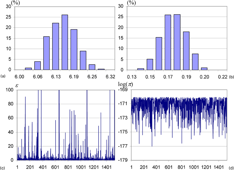
a sample distribution for α₁; b sample distribution for β₁; c trace of Hasting's ratio; d trace of log posteriors

OPEN IN VIEWER

Figure 3

Outputs from MCMC runs

The fitting of one fracture plane is effectively the same as the least squares fitting of a plane through the point cloud, which was calculated to be where (0·1593, −0·02317, −0·9870) are the directional cosines of the normal of the plane corresponding to a dip direction of 351·7° and a dip angle of 9·3° for the fitted plane. From samples obtained through the MCMC process, the dip direction and the dip angle of the plane have been estimated to be (the average values of the samples) 351·5 and 9·6° respectively. Clearly MCMC performs very well.

Baisch et al. (2006) use cross-correlation coefficients between waveforms to group the seismic events and they identify 613 clusters of events using the criterion of waveform cross-correlation coefficients >0·85. A total of 9176 events are included in these clusters with number of events in a cluster ranging from 2 to 158. Planes are then fitted to these clusters to improve the geometrical reservoir model. To mimic the fittings of these clusters, a fracture model consisting of 613 fractures using the following priors was generated:

The application of MCMC to update the fracture network used the following transition kernels:

The initial fracture model is shown in Fig. 4a. The fracture model after a million MCMC steps is given in Fig. 4b. For this model, numbers of seismic events associated with fracture planes range from 1 to 394, as shown in the distribution given in Fig. 5b. The distribution of d = {d_j:i}∀j is given in Fig. 5a. It is interesting to compare this distribution with the histogram of distances of relative hypocentre locations to layers determined separately for each cluster shown in Fig. 11 in Baisch et al. (2006) where 95% of the relative hypocentre locations are within ±25 m (estimated) from the layers. For the MCMC fracture model, this number is ±12 m, which indicates that the MCMC fracture model is a better fit. This is remarkable considering that no waveform correlation analysis is required and the difficulty of the model fitting was increased by taking into account all 23 232 seismic events while the model in Baisch et al. (2006) is based on only 9176 events. This also raises a concern about the assumption that seismic events with high cross-correlation coefficients belong to the same fracture (cluster) (Xu et al., 2011; Moriya et al. 2002).

OPEN IN VIEWER

Figure 4

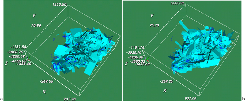
a initial model; b after optimisation

OPEN IN VIEWER

Figure 5

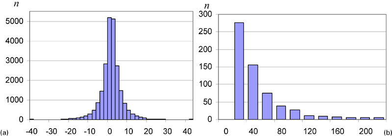
a distribution of d_j:i (m); b distribution of number of associations

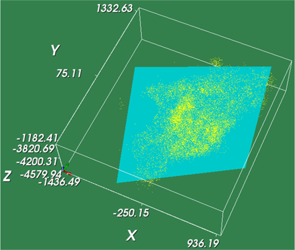
Fitted fracture plane ID286 has 394 associated seismic events which is the highest number. Figure 6a shows this particular fracture plane and its associated events. The distribution of distances of these seismic events to the plane is given in Fig. 6b. This fitted fracture plane covers an area of approximately 1×0·8 km and is dipping at 8° at an azimuth of 58°. The projection of the fitted fracture plane and its associated seismic events is shown in Fig. 7 which clearly demonstrates that the MCMC fitting process works very well. Baisch et al. (2006) describe a 140 seismic events cluster with a lateral extension of a few hundred metres. The 95% confidence interval based on distance to the layer plane has been estimated to be 6, 6 and 12 m respectively in easting, northing and elevation directions. For fracture ID286 in the model, the 95% confidence interval of the fitting based on distance to the fracture plane is [−14, 13] based on 394 values. Baisch et al. (2006) did not give sufficient detail for the 140 element cluster they analysed and therefore direct comparison of distances to the fitted plane is not possible.

OPEN IN VIEWER

Figure 6

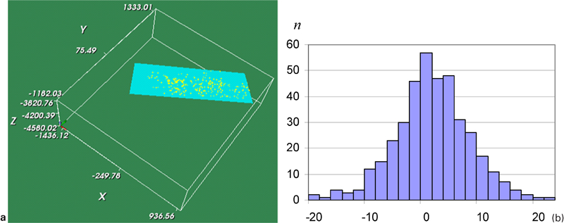
a fracture 286 and its associated points (m); b distribution of d_286:i (m)

OPEN IN VIEWER

Figure 7

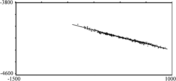
Point association with fracture 286 after optimisation, projected on plane perpendicular to the fracture plane and looking in down dip direction: vertical axis is exaggerated to give clearer view of point distribution

It is also interesting to examine the orientations of the fitted fracture planes. Figure 8 gives the pole projections of 613 fractures before and after the MCMC optimisation. Figure 8a is essentially the orientation distribution of the prior fracture model which shows a high degree of randomness. After optimisation (Fig. 8b), many fracture planes become subhorizontal. This result agrees well with the analysis done by Baisch et al. (2006) where fitted planes of 203 clusters (out of 613) were shown to have a dip angle less than 30°.

OPEN IN VIEWER

Figure 8

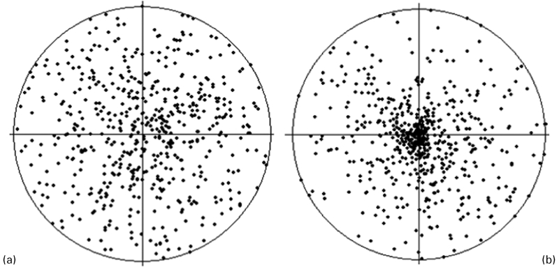
a initial model; b after optimisation

Conclusions

MCMC has been demonstrated to produce remarkably good results for fitting an optimised fracture model according to the specified criterion, both at the global scale and at the scale of an individual fracture. The model also confirms the subhorizontal features of fractures observed in the Habanero wells.

The technique described in this paper is statistical and no waveform correlation analysis was used. It is possible to combine the two techniques to improve the fitting. It is also possible to use non-planar polygons to fit the fracture model using the technique described. The fitted model is by no means the absolute best for Habanero reservoir. More models should be tested.