Incorporating waste management into oil sands long term production planning

Abstract

In oil sands mining, providing ore to the processing plant and tailings containment at the right time are the main drivers for profitability and sustainability. This paper introduces a mixed integer linear goal programming (MILGP) mine planning model to: determine the order and time of extraction of ore, dyke material and waste over the mine life that maximises the operation's net present value; and determine dyke material destination that minimises dyke construction cost. To implement an efficient MILGP model, an initial production schedule was generated and used as an input for the optimisation process. The model created value and a sustainable operation by generating a practical, smooth and uniform schedule for ore and dyke material. The total net present value generated including dyke construction cost for all pushbacks and destinations is $26 987M for a total mined tonnage of 7377 Mt.

Keywords

Oil sands mining Mixed integer linear goal programming Production scheduling optimisation Waste disposal planning Dyke construction

Introduction

A major aspect of mine planning is the optimisation of long term production scheduling. The aim of long term production scheduling usually is to determine the time and sequence of extraction and displacement of ore and waste in order to maximise the overall discounted net revenue from a mine within the existing economic, technical and environmental constraints. Long term production schedules define the mining and processing plant capacity and expansion potential, as well as management investment strategy. In mining projects, deviations from optimal mine plans will result in significant financial losses, future financial liabilities, delayed reclamation and resource sterilisation.

Mixed integer linear goal programming (MILGP) mathematical models are considered powerful tools in optimising mine production schedules and there have been some efforts in applying them to mining projects. Though mathematical programming models (MPMs) have been applied in mine production scheduling, very little work has been carried out in terms of oil sands mine planning, which has a unique scenario when it comes to waste management. Recent mining regulations by Alberta Energy Resources and Conservation Board (Directive 074) (McFadyen, 2008) require oil sands mining companies to develop integrated mine planning and waste management strategies for their in-pit and external tailings facilities. The MILGP model used for this research incorporates multiple material types with multiple elements for multiple destinations in oil sands long term production planning (OSLTPP). This MILGP model however results in a large scale optimisation problem which may become intractable or have long solution times. The objective of this paper is to develop and verify an efficient MILGP model for OSLTPP and waste management that delivers practical results in a reasonable time.

Oil sands mining is increasingly becoming challenging as oil sands companies integrate responsible socio-environmental waste management practices into their operations. Together with the limitations in lease areas, it has become necessary to look into effective and efficient waste disposal planning system. This system should be well integrated into the long term mine plan in an optimisation framework that creates value and a sustainable operation. In oil sands operations, the pit phase mining occurs simultaneously with the construction of in-pit dykes in the mined out areas of the pit and ex-pit dykes in designated areas outside the pit. These dykes are constructed to hold tailings that are produced during processing of the oil sands ore. The materials used in constructing these dykes come from the oil sands mining operation. The dyke materials are made up of overburden (OB), interburden (IB) and tailings coarse sand (TCS). Any material that does not qualify as ore or dyke material is sent to the waste dump.

In implementing an efficient MILGP model to incorporate waste management into OSLTPP, our targets are to:

determine the order and time of extraction of ore, dyke material and waste to be removed from a predefined final pit limit over the mine life that maximises the net present value (NPV) of the operation

ii.

determine the destination of dyke material that minimises construction cost based on the construction requirements of the various dykes.

Before OSLTPP, we assume that the material in the final pit limit is discretised into a three-dimensional array of rectangular or cubical blocks called a block model. Attributes of the material in the block model such as rock types, densities, grades, or economic data are represented numerically. Figure 1 shows the schematic representation of the problem definition containing K mining-cuts. Mining-cuts are clusters of blocks within the same level or mining bench that are grouped based on a similarity index defined using the attributes; location, grade, rock type and the shape of mining-cuts that are created on the lower bench. In this research, an agglomerative hierarchical clustering algorithm which seeks to generate clusters with reduced mining-cut extraction precedence is used (Tabesh and Askari-Nasab, 2011). Each mining-cut k, is made up of ore o_k, OB dyke material d_k, IB dyke material n_k and waste w_k. The material in each mining-cut is to be scheduled over T periods depending on the goals and constraints associated with the mining operation. Overburden dyke material scheduled , IB dyke material scheduled and TCS dyke material from the processed ore scheduled , must further be assigned to the dyke construction sites based on construction requirements. For period t₁, the dyke construction material required by site i is dyke_i. In addition, the final pit limit block model is divided into pushbacks. The material intersecting a pushback and a bench is known as a mining-panel. Each mining-panel contains a set of mining-cuts and is used to control the mine production operation sequencing.

Figure 1

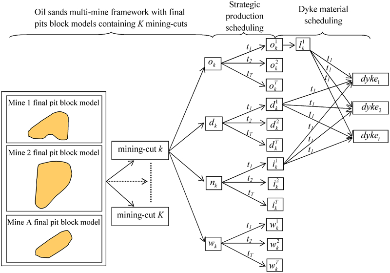
Schematic representation of problem definition showing strategic production and dyke material scheduling modified after Ben-Awuah and Askari-Nasab (2011)

The schedules generated for OSLTPP drives the profitability and sustainability of an oil sands mining operation. The strategic production and dyke material schedules control the NPV of the operation and provide the platform for a robust waste management planning strategy. Lack of proper waste management planning can lead to environmental and sustainability issues resulting in major financial liabilities or immediate mine closure by regulatory agencies.

The rest of the paper is organised as follows. The section on ‘Summary of literature review’ summarises the literature on the application of MPMs to the long term production planning (LTPP) problem. This is followed by a section on the application of MILGP model for OSLTPP and waste management. The section on ‘Implementation of efficient MILGP model for OSLTPP and waste management’ outlines the implementation of an efficient MILGP model for OSLTPP and waste management and a case study presented in the section on ‘Case study: implementation of MILGP model’. This paper concludes in the section on ‘Conclusions’.

Summary of literature review

Applying MPMs like linear programming (LP), mixed integer linear programming (MILP) and goal programming with exact solution methodologies have proved to be robust. Solving MPMs with exact solution methodologies result in solutions within known limits of optimality. As the solution gets closer to optimality, it results in production schedules that generate higher NPVs than those obtained from heuristic optimisation methods. This has resulted in extensive research on the application of MPMs like LP and MILP to the LTPP problem. The inherent difficulty in applying these models to the LTPP problem is that, they result in large scale optimisation problems containing many binary and continuous variables. These are difficult to solve with the current computing software and hardware available and may have lengthy solution times. Though some researchers have made efforts in reducing the solution time associated with solving MPMs, their models were deficient in terms of dealing with large block model sizes or could not generate feasible practical mining strategies. These publications note that the size of the resulting LP and MILP models is a major problem, because it contains too many binary and continuous variables (Johnson, 1969; Gershon, 1983; Dagdelen, 1985; Akaike and Dagdelen, 1999; Ramazan, 2001; Caccetta and Hill, 2003; Ramazan and Dimitrakopoulos, 2004).

Goal programming is another mathematical programming modelling platform that have been used in solving the LTPP problem. It permits flexible formulation, specification of priorities among goals, and some level of interactions between the decision maker and the optimisation process (Zeleny, 1980; Hannan, 1985). This leads to its application to the LTPP problem by Zhang et al. (1993), Chanda and Dagdelen (1995) and Esfandiri et al. (2004). They were, however, unable to practically implement their models due to the numerous mining production constraints and size of the optimisation problem. Recent implementation of MILP models with block clustering techniques were successfully undertaken for an iron ore deposit (Askari-Nasab et al., 2010, 2011). It, however, lacks the framework for the implementation of an integrated mine planning and waste management system as is the case required for sustainable oil sands mining. Owing to the strategy required for sustainable oil sands mining and the regulatory requirements from Directive 074, waste disposal planning is closely related to the mine planning system (McFadyen, 2008; Askari-Nasab and Ben-Awuah, 2011; Ben-Awuah and Askari-Nasab, 2011). Currently, oil sands waste disposal planning is handled as a post-production scheduling optimisation activity. Modelling an integrated mine planning system even adds more complexity to the LTPP problem. Ben-Awuah et al. (2012) has implemented a MILGP model for an integrated oil sands production scheduling and waste disposal planning system. The model takes into account multiple material types, elements and destinations, directional mining, waste management and sustainable practical mining strategies. The implementation of the MILGP model resulted in a large-scale optimisation problem with lengthy solution times.

This paper presents scheduling models and tests on how to generate MILGP formulations using fewer non-zero decision variables. It also discusses alternative techniques to MILGP pushback mining modelling for efficiency in solving the formulations. The tests show that there are significant differences in the time taken by the various MILGP models generated for the same deposit to maximise NPV and minimise dyke construction cost. An oil sands multi mine data set is used for the case study.

Model for OSLTPP and waste management by MILGP

The OSLTPP and waste management problem is to find the time and sequence of extraction of ore, dyke material and waste mining-cuts to be removed from predefined open pit outlines and their respective destinations over the mine life, so that the NPV of the operation is maximised and dyke construction cost is minimised. In general, the MILGP formulation is for multiple material types and destinations, as well as pushbacks which ties into the waste management strategy for oil sands operations. The production schedule is subject to a variety of technical, physical and economic goals, and constraints which enforce mining extraction sequence, mining and dyke construction capacities, and blending requirements. The notations used in the formulation of the OSLTPP and waste management problem have been classified as sets, indices, parameters and decision variables. The details of these notations can be found in the Appendix.

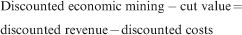
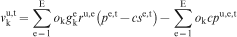
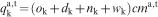
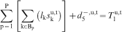
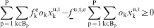
The summary of economic data for each mining-cut known as economic mining-cut value is based on ore parcels within mining-cuts which could be mined selectively. The economic mining-cut value is a function of the value of the mining-cut based on the processing destination and the costs incurred in mining from a designated location and processing, and dyke construction at a specified destination. The cost of dyke construction is also a function of the location of the tailings facility being constructed and the type and quantity of dyke material used. The discounted economic mining-cut value for mining-cut k is equal to the discounted revenue obtained by selling the final product contained in mining-cut k minus the discounted cost involved in mining mining-cut k as waste minus the extra discounted cost of mining OB and IB dyke material, and generating TCS dyke material from mining-cut k for a designated dyke construction destination. This can be summarised by equations (1)–(6). The discounted economic mining-panel value is the sum of the discounted economic mining-cut value of all the mining-cuts belonging to that mining-panel. (1) The parameters in equation (1) can be defined by equations (2)–(6) (2) (3) (4) (5) (6)

Objective functions of MILGP model

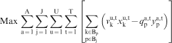
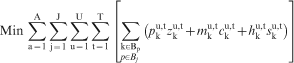
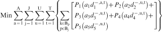
The objective functions of the MILGP model for OSLTPP and waste management can be formulated as:

maximising the NPV of the mining operation

ii.

minimising the dyke construction cost for the waste management plan

iii.

minimising the deviations from the set goals.

We used the concepts presented in Ben-Awuah et al. (2012) as the starting point of our development. The formulation uses continuous decision variables, , , , and to model mining and processing requirements, and OB, IB and TCS dyke material requirements respectively, for all mining locations and processing and dyke construction destinations. Using continuous decision variables allows for fractional extraction of mining-panels and mining-cuts in different periods for different locations and destinations. 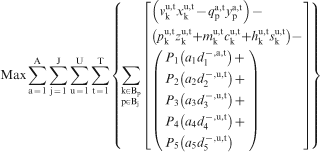Continuous deviational variables, , , , and have been defined to support the goal functions that control mining, processing, OB, IB and TCS dyke material, for all mining locations and processing and dyke construction destinations. The deviational variables provide a continuous range of units (t) that the optimiser can choose from to satisfy the set goals. In the objective function, these deviational variables are minimised. The objective function also contains deviational penalty cost and priority (PP) parameters. The deviational penalty cost parameters, a₁, a₂, a₃, a₄ and a₅, penalises the NPV for any deviation from the set goals. The priority parameters, P₁, P₂, P₃, P₄ and P₅, are used to place emphasis on the goals that are more important. The PP parameters are set up to penalise the NPV if the set goals are not met as well as the most important goal.

When setting up these parameters, the planner needs to monitor how continuous mining proceeds period by period and the uniformity of tonnages mined per period, as well as the corresponding NPV generated, to keep track of how parameter changes affect these key performance indicators. In some scenarios, the limit for setting the PP parameters depends on the extent to which the planner wants to trade off NPV to meet the set goals. A higher PP parameter may enforce a goal to be met whilst reducing the NPV of the operation. A case showing this trend was analysed in Ben-Awuah et al. (2012). In general, the magnitude of the PP parameters should be calibrated based on the objectives of management. More weight should be assigned to a goal that has a higher priority for the management.

The three objective functions of the MILGP model for OSLTPP and waste management are represented by equations (7)–(9) (7) (8) (9) Equations (7)–(9) can be combined as a single objective function formulated as in equation (10) (10)

Goal functions of MILGP model

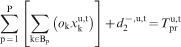
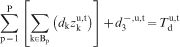
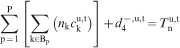
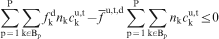
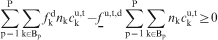
In the proposed model, the goals to be achieved are the mining and processing targets, and OB, IB and TCS dyke materials targets in tonnes for all mining locations, and processing and dyke construction destinations. These goal functions are represented by equations (11)–(15) (11) (12) (13) (14) (15) Equation (11) represents the mining goal function which ensures the total amount of ore, dyke material and waste mined in each period from all mining locations equals the total available equipment capacity with a defined acceptable deviation. Equation (12) represents the processing goal function which controls the mill feed. This goal helps the mine planner to provide a uniform feed throughout the mine life resulting in an effectively integrated mine-to-mill operation. Equations (13)–(15) represent the dyke material goal functions which control dyke construction scheduling. These goals enable the mine planner to schedule the required dyke materials for all dyke construction destinations. The TCS dyke material generated from the processing plant is directly dependent on the mill feed.

Grade blending constraints of MILGP model

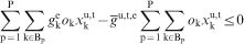
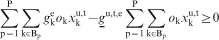
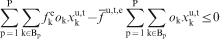
The MILGP model grade blending constraints control the grade of ore bitumen, ore fines and IB fines in the mined material for all processing and dyke construction destinations. These constraints are formulated by equations (16)–(21) (16) (17) (18) (19) (20) (21) Equations (16)–(19) represent inequality constraints which monitor the mill feed quality. They specify the limiting grade requirements for ore bitumen and ore fines for processing. Equations (20) and (21) represent inequality constraints that control the IB dyke material quality. They specify the limiting grade requirements for IB dyke material fines for dyke construction. Among other things, the dyke material quality defines the integrity of the tailings containment facilities constructed.

Variables control constraints of MILGP model

In the proposed model, the variables control constraints monitor the logics of the variables that define mining, processing, dyke materials and goal deviations to ensure they are within acceptable ranges. These variables control constraints are represented by equations (22)–(29) (22) (23) (24) (25) (26) (27) (28) (29) Equation (22) outlines inequalities that ensure that the total material mined from mining-panel p in any given scheduling period from any mining location exceeds or is equal to the sum of the ore and OB and IB dyke material mined from the mining-cuts belonging to that mining-panel. It is assumed that when a mining-panel is scheduled, all the mining-cuts, blocks or parcels within the mining-panel are extracted uniformly. Equation (23) states that the fraction of TCS dyke material produced in each period should be less or equal to the fraction of ore mined for all destinations. This constraint manages the direct relationship between ore and TCS dyke material. TCS dyke material is only generated when ore is processed for bitumen extraction. Equations (24)–(28) ensure that the total fractions of mining-panel p and mining-cut k mined and TCS dyke material produced and sent to all destinations in all periods is less or equal to one. This keeps track of the different portions of mining-panels and mining-cuts that are scheduled for various destinations. Equation (29) defines the non-negativity of the deviational variables defined to support the goal functions.

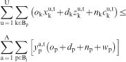
Mining-panels extraction precedence constraints of MILGP model

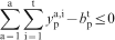
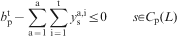
The mining-panels extraction precedence in the MILGP model is defined by equations (30)–(34). Binary integer decision variable is used to control precedence of mining-panels extraction. is equal to one if the extraction of mining-panel p has started by or in period t, otherwise it is zero. These equations together implement the vertical and horizontal mining-panel extraction sequence. (30) (31) (32) (33) (34) For each mining-panel p, equations (30)–(34) check the set of immediate predecessor mining-panels that must be mined before mining mining-panel p for all periods and from all locations. This precedence relationship ensures that:

all the immediate predecessor mining-panels above the current mining-panel p are extracted before extraction of mining-panel p; represented by the set C_p(L)

ii.

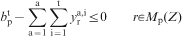
all the immediate predecessor mining-panels preceding the current mining-panel p in the horizontal mining direction are extracted before extraction of mining-panel p; represented by the set M_p(Z)

iii.

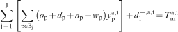
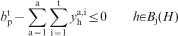
all the mining-panels within the immediate predecessor mining phase that precedes the current mining phase, j are extracted before extraction of mining-panel p in the current mining phase; represented by the set B_j(H).

Implementation of efficient MILGP model for OSLTPP and waste management

We have progressively developed an efficient and robust MILGP model for solving the OSLTPP and waste management problem which involves multiple destinations, material types, mining locations and pushbacks (Askari-Nasab and Ben-Awuah, 2011; Ben-Awuah and Askari-Nasab, 2011). This leads to a large scale optimisation problem with numerous decision variables and constraints that takes large memory overheads and time to solve, thus resulting in a sophisticated production scheduling problem which calls for improved numerical modelling and optimisation techniques to deliver acceptable results in a timely manner. We have further developed techniques to reduce the number of non-zero decision variables and pushback mining constraints in the production scheduling problem. We also implemented a practical mine production sequencing with mining-panels which results in reduced number of binary variables to be solved during optimisation. The formulated MILGP production scheduling problems are solved using Tomlab/CPLEX (Holmström et al., 2009).

Implementation of MILGP with fewer non-zero decision variables

The main set-back in solving large scale MILGP problems is the size of the branch and cut tree. During optimisation, the size of the branch and cut tree becomes so large that insufficient memory remains to solve an LP subproblem. The size of the branch and cut tree depends on the number of decision variables in the formulation. The general strategy in formulating the MILGP for OSLTPP and waste management is therefore to reduce the number of decision variables in the production scheduling problem, thereby reducing the solution time significantly. This is implemented using an initial production schedule generated based on a practical oil sands directional mining strategy and the annual mining capacity.

The general form of the MILGP formulation can be represented by equation (35) as (35) subject to: goals and constraints of the MILGP model.

The objective function for the OSLTPP problem as stated by equation (10) maximises the NPV and minimises the dyke construction cost. The objective function coefficient vector c is a column vector containing the discounted revenue and cost values for all mining-panels and mining-cuts in all periods and for all destinations. This is shown by equation (36). The objective function decision variables vector r is a column vector containing mining-cut or mining-panel precedence, ore, mining, OB, IB and TCS production and deviational variables. This is shown by equation (37). The notations used have been defined in the Appendix. The decision variables vector r is therefore made up of 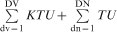non-zero decision variables to be solved for in the MILGP model during optimisation. This vector ensures that each mining-cut or mining-panel is available for production scheduling during the entire mine life. As shown in the section on ‘Generating and applying initial production schedule’, by having an initial production schedule, the number of non-zero decision variables in r can be reduced, thereby reducing the size of the production scheduling problem. 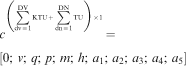(36) (37) where are the decision variables in the objective function; are the deviational variables in the objective function; and K is the number of mining-cuts or mining-panels involved depending on the coefficient or variable being set up.

Generating and applying initial production schedule

This technique is based on a practical directional oil sands mining and the continuous depletion of material from a given mining and processing capacity. An initial production schedule can be generated using a fast heuristic production scheduling algorithm like Whittle's Fixed Lead algorithm (Gemcom Software International, 2012) or a moving production bin calculated estimate. Before optimisation with the MILGP model, Whittle can be used to generate a production schedule and then some periodic tolerance applied to the schedule and used as an initial production schedule. Similarly, a moving production bin can be initiated at one end of the deposit and with the annual mining and processing targets and mining direction, a schedule can be generated. Applying a periodic tolerance, an initial schedule can be generated for the MILGP model as well.

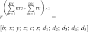
Let us consider an oil sands deposit containing 980 mining-cuts in two pushbacks which is to be mined from west to east over 12 periods for the processing plant and four dyke construction destinations, as shown in Fig. 2. The production scheduling and waste disposal planning strategy to be used here is based on a practical directional oil sands mining similar to the conceptual mining model implemented by Askari-Nasab and Ben-Awuah (2011). This includes complete extraction of pushback 1 before the mining of pushback 2 to ensure that pushback 1 can be used for tailings disposal planning. From Fig. 2, based on the mining and processing goals and direction of mining we can estimate that mining-cut 6 may be mined in, say, period 4. Assuming we apply a periodic tolerance of 3, then in the initial schedule for the MILGP model, mining-cut 6 can be said to be extractable over periods 1–7, while the rest of the periods are set to zeros. Conventionally, mining-cut 6 will have been modelled to be extractable over the entire 12 years mine life. With this technique, the number of non-zero decision variables, r to be solved for in the MILGP model during production scheduling will reduce from 176 568 to 94 472. This reduces the size of the production scheduling problem significantly.

Figure 2

Schematic representation of oil sands deposit showing mining-cuts and pushbacks

Theoretically, this variable reduction technique decreases the solution space for the optimisation problem. Thus during optimisation, some of the branches in the branch and cut tree are eliminated, ensuring that the solution for the practical production scheduling problem is reached faster. It is important to note that, reducing the solution space unreasonably can cause one to miss the optimal practical production scheduling solution. This method must be applied in accordance to the mining and processing capacities defined.

Multimine implementation of MILGP with fewer pushback mining precedence constraints

In OSLTPP and waste management, it is important to have a pushback mining precedence strategy that ties into the waste disposal plan. This requires the development of a well integrated strategy of directional and pushback mining, and tailings dyke construction for in-pit and ex-pit tailings storage management. This includes the complete extraction of one pushback before the mining of the next pushback in the direction of mining, thus enabling the release of the dyke footprints of the recently mined pushback for dyke construction to start and then subsequently tailings deposition. Details of this integrated mine planning and waste management strategy has been well documented by Askari-Nasab and Ben-Awuah (2011). Multiple mines final pits are modelled as pushbacks and the MILGP model applied appropriately.

To implement the complete extraction of pushbacks during optimisation, pushback mining precedence constraints must be developed and implemented whilst ensuring that the optimisation problem is still feasible within a reasonable time. This requires an efficient modelling of the pushback mining precedence constraints to reduce the number of variables being added to the problem. The strategy used by the MILGP model has been tied into the vertical and horizontal extraction precedence constraints of the mining-panels. Three cases and strategies have been identified and are illustrated in Fig. 3.

Figure 3

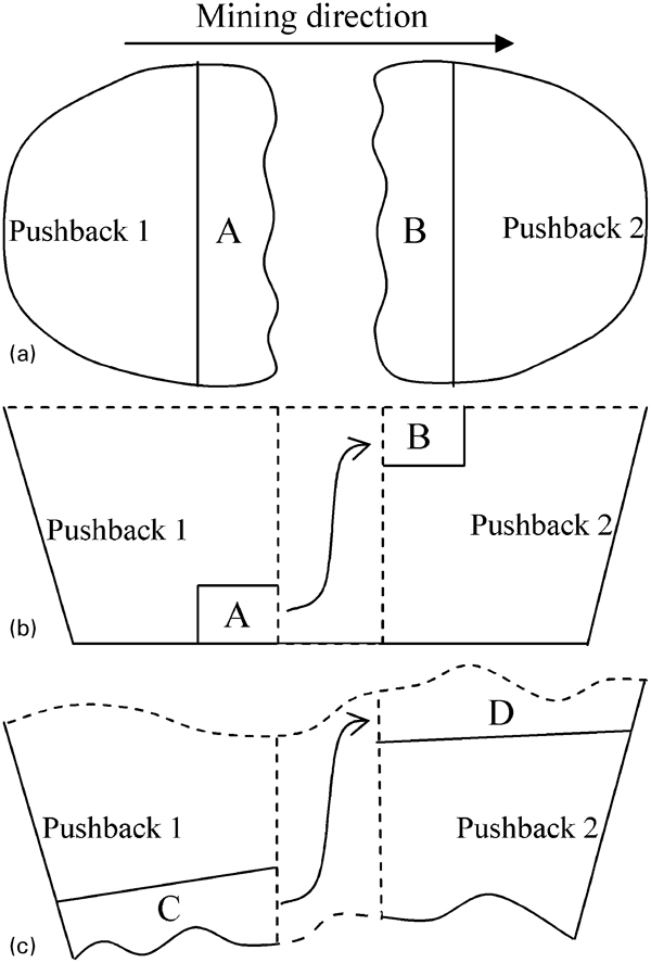
Developing pushback mining precedence constraints

The first case in Fig. 3a and b assumes that pushbacks in the final pit being used as an input for the MILGP model has flat topography and bottom. This means that with the west to east mining direction, mining will proceed in pushback 1 until it reaches the bottom of the pit where the list of bounding mining-panels in set A becomes the last set of mining-panels for complete extraction of pushback 1 before pushback 2. Set B also contains the list of bounding mining-panels at the top of pushback 2 where mining starts. Set A therefore becomes the preceding mining-panels set to set B. The pushback mining precedence constraints here involves identifying the list of bounding mining-panels that belongs to sets A and B and applying the mining-panels extraction precedence constraints in equations (32)–(34).

The second case in Fig. 3c is when the final pit has undulating topography and bottom which is almost always the case. Here, we look for set C which is made up of the bounding mining-panels at the bottom of pushback 1 mined last. Set D also contains the list of bounding mining-panels at the top of pushback 2 which must be mined first when mining of pushback 2 starts. This approach becomes necessary because the mining-panels at the bottom of pushback 1 and top of pushback 2 belong to different mining benches therefore the vertical and horizontal mining-panels extraction precedence constraints are not able to tie the mining of these mining-panels together. Set C becomes the preceding mining-panels set to set D. Similarly, the mining-panels extraction precedence constraints in equations (32)–(34) can then be applied to implement the complete extraction of pushback 1 before pushback 2.

The third case is when you have a similar situation in Fig. 3c. The strategy here is by adding air mining-panels to the final pit both at the top and bottom, converting it from case 2 to case 1. Case 1 strategy can then be applied to implement the pushback mining precedence constraints.

The strategy used in the second case was implemented in the case study in this paper.

Case study: implementation of MILGP model

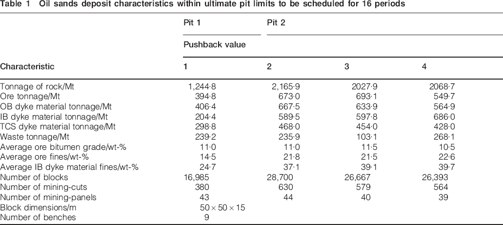
The MILGP model was coded in Matlab (Mathworks Inc., 2011) and implemented on an oil sands deposit which has two final pits covering an area of about 3900 ha. The mineralised zone of this deposit occurs in the McMurray formations. The deposit is to be scheduled for 16 periods equivalent to 16 years for the processing plant and dyke construction destinations. The performance of the proposed MILGP model was analysed based on NPV, mining production goals, smoothness and practicality of the generated schedules, the availability of tailings containment areas at the required time and the computational time required for convergence. The model was implemented on a Quad-Core Dell Precision T7500 computer at 2·8 GHz, with 24 GB of RAM. Table 1 provides information about the orebody model within the ultimate pits limits used in the case study.

Table 1

Oil sands deposit characteristics within ultimate pit limits to be scheduled for 16 periods

Characteristic	Pit 1	Pit 2
	Pushback value
	1	2	3	4
Tonnage of rock/Mt	1,244·8	2,165·9	2027·9	2068·7
Ore tonnage/Mt	394·8	673·0	693·1	549·7
OB dyke material tonnage/Mt	406·4	667·5	633·9	564·9
IB dyke material tonnage/Mt	204·4	589·5	597·8	686·0
TCS dyke material tonnage/Mt	298·8	468·0	454·0	428·0
Waste tonnage/Mt	239·2	235·9	103·1	268·1
Average ore bitumen grade/wt-%	11·0	11·0	11·5	10·5
Average ore fines/wt-%	14·5	21·8	21·5	22·6
Average IB dyke material fines/wt-%	24·7	37·1	39·1	39·7
Number of blocks	16,985	28,700	26,667	26,393
Number of mining-cuts	380	630	579	564
Number of mining-panels	43	44	40	39
Block dimensions/m	50×50×15
Number of benches	9

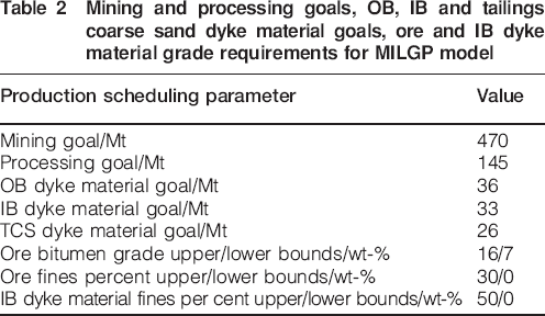
The area to be mined are divided into four pushbacks in consultation with tailings dam engineers based on required tailings cell capacities and the timelines required in making the cell areas available for tailings containment. These four pushbacks are further divided into 20 intermediate pushbacks to enable the creation of practical mining-panels to be used in controlling the mining operation. These intermediate pushbacks are created using an approximately equal distribution of tonnages to be mined across the deposit. An agglomerative hierarchical clustering algorithm is used in clustering blocks within each intermediate pushback into mining-cuts (Tabesh and Askari-Nasab, 2011). Clustering blocks into mining-cuts ensures the MILGP scheduler generates a mining schedule at a selective mining unit that is practical from mining operation perspective. In solving the MILGP model with CPLEX, the absolute tolerance on the gap between the best integer objective and the objective of the best node remaining in the branch and cut algorithm, referred to as EPGAP, was set at 5% for the optimisation of the mining project. The mining targets, processing plant feed, dyke construction requirements, bitumen grade and fines percent need to be controlled within acceptable ranges. These requirements have been summarised in Table 2. Mining will proceed generally from west to east; from pushback 1 to 4 with complete extraction of each pushback before the next. In addition to the processing plant, dyke material requirements for four dyke construction destinations will be scheduled simultaneously. It is assumed that all dyke construction destinations are ready to receive dyke material as soon as mining starts. Details of the waste management strategy implemented here has been well documented by Askari-Nasab and Ben-Awuah (2011).

Table 2

Mining and processing goals, OB, IB and tailings coarse sand dyke material goals, ore and IB dyke material grade requirements for MILGP model

Production scheduling parameter	Value
Mining goal/Mt	470
Processing goal/Mt	145
OB dyke material goal/Mt	36
IB dyke material goal/Mt	33
TCS dyke material goal/Mt	26
Ore bitumen grade upper/lower bounds/wt-%	16/7
Ore fines percent upper/lower bounds/wt-%	30/0
IB dyke material fines per cent upper/lower bounds/wt-%	50/0

Analysis

Run 2 was chosen for analysis due to its significantly reduced solution time. After optimisation, the overall NPV generated including the dyke construction cost for all pushbacks and destinations is $26 987M and the total dyke construction cost is $3821M at a 4·98% EPGAP. The scenario implemented here focuses on a practically integrated OSLTPP and waste management strategy that generates value and sustainability. This includes mining in a specified direction and making completely extracted pushbacks available for in-pit dyke construction and subsequently tailings management. This reduces the environmental footprints of the external tailings facility by commissioning in-pit tailings facilities when the active pushback is completely mined. The mining direction was decided on during the initial production schedule run using the Fixed Lead heuristic algorithm in Whittle (Gemcom Software International, 2012). The mining direction with the best NPV was selected for the MILGP model. The mining sequence at level 305 m for all pushbacks with a west–east mining direction can be seen in Fig. 4. Figure 4 also shows the complete extraction of each pushback before mining the next, to support tailings management. The mining sequence shows a progressive continuous mining in the specified direction to ensure least mobility and increased utilisation of loading equipments. This is very important in the case of oil sands mining where large cable shovels are used. The size of the mining-cuts and mining-panels also enables good equipment maneuverability and supports multiple material loading operations. The mining-panels enable mining to proceed with a reduced number of required drop-cuts. Using mining-cuts to schedule for processing plant and dyke construction also allows for flexible and practical ore and dyke material selective mining that supports our preferred run-of-mine blending.

Figure 4

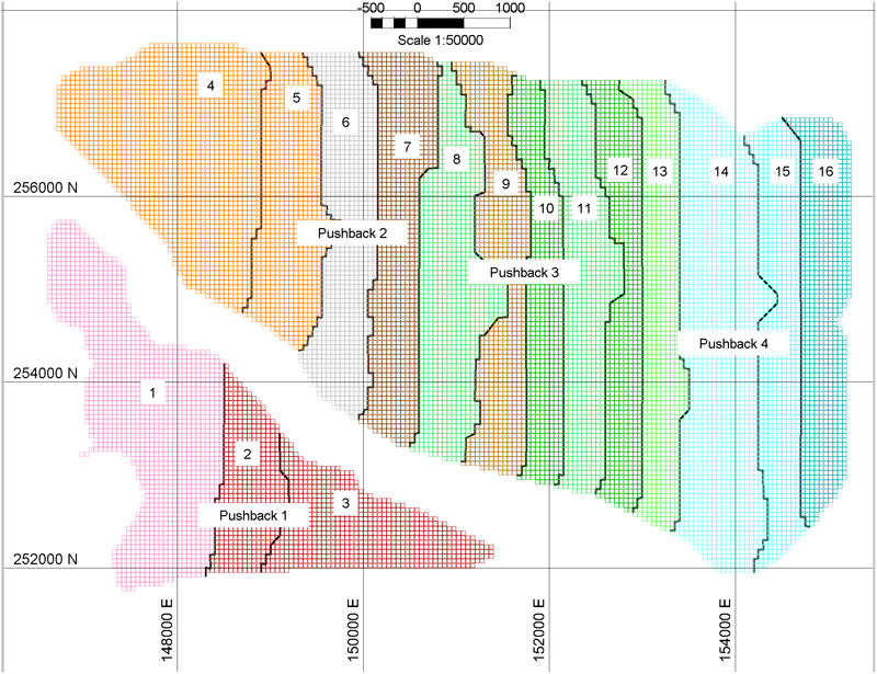
Mining sequence at level 305 m for all pushbacks with west–east mining direction

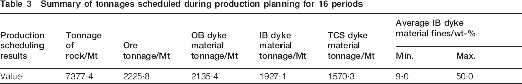
Figure 5 shows uniform mining and processing schedules that ensures efficient utilisation of mining fleet and processing plant capacity throughout the mine life. The schedule provides the quality and quantity of dyke material needed to build the dykes of the external tailings facility and in-pit tailings cells in a timely manner and at a minimum cost. Pre-stripping of pushback 1 and 2 starts in the first and fourth years, resulting in less ore being mined. Subsequently, uniform ore feed is provided at the required processing plant capacity throughout the mine life. The dyke material mined is sent to the scheduled dyke construction destination. Table 3 shows the total material mined, ore, OB and IB dyke material tonnage mined and TCS dyke material tonnage generated from the processing plant. The schedules give the planner good control over dyke material and provides a robust platform for effective dyke construction planning and tailings storage management.

Figure 5

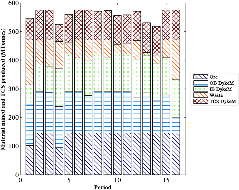
Schedules for ore, OB, IB and tailings coarse sand dyke material, and waste tonnages

Table 3

Summary of tonnages scheduled during production planning for 16 periods

Production scheduling results	Tonnage of rock/Mt	Ore tonnage/Mt	OB dyke material tonnage/Mt	IB dyke material tonnage/Mt	TCS dyke material tonnage/Mt	Average IB dyke material fines/wt-%
Production scheduling results	Tonnage of rock/Mt	Ore tonnage/Mt	OB dyke material tonnage/Mt	IB dyke material tonnage/Mt	TCS dyke material tonnage/Mt	Min.	Max.
Value	7377·4	2225·8	2135·4	1927·1	1570·3	9·0	50·0

The ore and dyke material quality is obtained by blending the run-of-mine material. The targeted processing plant head grade and IB dyke material grade that was set were successfully achieved in all periods and for all destinations. We targeted to reduce the periodic grade variability by setting tighter lower and upper grade bounds. The periodic grades in each pushback can be varied depending on the processing plant or dyke construction requirements whilst ensuring a feasible solution is obtained. Figures 6 and 7 show the average ore bitumen grades and ore fines percent over the mine life. The average IB dyke material fines percent range obtained for all destinations has been summarised in Table 3.

Figure 6

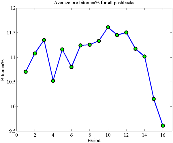
Average ore bitumen grades in all periods

Figure 7

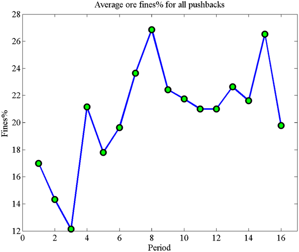
Average ore fines percentage in all periods

Comparison

In implementing the efficient MILGP model with fewer non-zero decision variables, two optimisation scenarios were executed to assess our model. Table 4 shows a summary of the results of the scenarios with different number of decision variables remaining before and after applying an initial schedule with a periodic tolerance. The results show <1% change in NPV and >99% change in solution time due to differences in solution space. Run 1 have a lower NPV due to the increase in dyke material tonnage and the associated waste material mined. This resulted in a higher tonnage mined in run 1. The results also show run 2 terminating at a branch closer to the optimal solution than run 1 as shown by the EPGAP. The ore tonnages sent to the processing plant in the two scenarios were the same. However there is a significant decrease in the CPU time as the number of decision variables are reduced using the initial schedule with a periodic tolerance. After applying a periodic tolerance of 2, the number of decision variables in run 1 reduced from 453 360 to 121 884, while the CPU time reduced from 243·79 to 0·84 h which represents over 99% decrease in solution time for run 2. This technique can be used to overcome the long CPU time associated with solving mathematical models like the MILGP model thus bringing its daily use to the front due to its advantages. For a chosen application, the periodic tolerance required to be applied to an initial schedule from a heuristic could be established and used appropriately each time.

Table 4

Summary of results before and after applying initial schedule with periodic tolerance

Run no.	Periodic tolerance/years	No. of decision variables	NPV/M$	Tonnage mined/Mt	Ore tonnage/Mt	Dyke material tonnage/Mt	EPGAP/%	CPU time/hrs
1	…	453 360	26 791	7504·6	2225·8	5654·2	5·00	243·79
2	2	121 884	26 987	7377·4	2225·8	5632·8	4·98	0·84

In general, it should be noted that the solution time for MILGP models do not depend only on the number of decision variables, but also on the tightness of the model which includes the data set used, the objective function and the constraints. The data used determine the coefficients in the objective function, and coefficients and bounds of the goals and constraints which have major impact on the solution time of an MILGP model.

Conclusions

We have developed, implemented and verified a MILGP formulation which takes into account practical shovel movements by selecting mining-panels and mining-cuts that are comparable to the selective mining units of oil sands mining operations. Different techniques have been presented for implementing an efficient MILGP model that serves as a guide for optimisation of OSLTPP and waste management. The model created value and a sustainable operation by generating a practical, smooth and uniform schedule for ore and dyke material. The schedule gives the planner good control over dyke material and provides a robust platform for effective dyke construction and waste disposal planning. The schedule ensures that the major factors affecting oil sands profitability and sustainability are taken care of within an optimisation framework by maximising NPVs while creating timely tailings storage areas.

It has been shown that using an initial schedule with a periodic tolerance results in reduced number of decision variables to be solved in the production scheduling problem. This variable reduction technique reduced the CPU time by >99%, changing the long CPU times associated with solving mathematical models like the MILGP. In addition to its advantages, the reduced solution time will make the use of such mathematical models more appealing in solving mine planning problems. For a chosen application, the periodic tolerance required to be applied to an initial schedule from a heuristic could be established and used appropriately each time.

The total NPV generated including dyke construction cost for all pushbacks and destinations is $26 987M. The average bitumen grade for the scheduled ore was 11·0%. The average ore and IB dyke material fines percent ranges between 12·1 and 26·9, and 9 and 50 respectively. The total material mined was 7377 Mt, which includes: 2226 Mt ore; 2135 Mt OB dyke material and 1927 Mt IB dyke material whilst 1570 Mt of TCS dyke material was generated from the processing plant.

Footnotes

Appendix

References

Akaike

, Dagdelen

1999. A strategic production scheduling method for an open pit mine, Proc. 28th Int. Symp. on ‘The application of computers and operations research in the mineral industry’, 729–738; Golden, CO, Colorado School of Mines.

Askari-Nasab

, Awuah-Offei

, Eivazy

2010. Large-scale open pit production scheduling using mixed integer linear programming, Int. J. Min. Miner. Eng., 2, (3), 185–214.

Askari-Nasab

, Ben-Awuah

2011. Integration of oil sands mine planning and waste management using goal programming, Proc. 35th Int. Symp. on ‘The application of computers and operations research in the mineral industry’, 329–350; Carlton Vicotia, Wollongong, The Australasian Institute of Mining and Metallurgy.

Askari-Nasab

, Pourrahimian

, Ben-Awuah

, Kalantari

2011. Mixed integer linear programming formulations for open pit production scheduling, J. Min. Sci., 47, (3), 338–359.

Ben-Awuah

, Askari-Nasab

2011. Oil sands mine planning and waste management using mixed integer goal programming, Int. J. Min. Reclam. Environ., 25, (3), 226–247.

Ben-Awuah

, Askari-Nasab

, Awuah-Offei

2012. Production scheduling and waste disposal planning for oil sands mining using goal programming, J. Environ. Inform., 20, (1), 20–33.

Caccetta

, Hill

. 2003. An application of branch and cut to open pit mine scheduling, J. Global Optim., 27, (2–3), 349–365.

Chanda

EKC

, Dagdelen

, 1995. Optimal blending of mine production using goal programming and interactive graphics systems, Int. J. Min. Reclam. Environ., 9, (4), 203–208.

Dagdelen

, 1985. Optimum multi-period open pit mine production scheduling by Lagrangian parameterization, PhD thesis, University of Colorado, Golden, CO, USA.

10.

Esfandiri

, Aryanezhad

, Abrishamifar

. 2004. Open pit optimization including mineral dressing criteria using 0-1 non-linear goal programming,. Trans Insti. Min. Metall. A, 113A, (1), 3–16.

11.

Gemcom Software International . 2012. Gemcom GEMS, Ver 6.3, Vancouver.

12.

Gemcom Software International . 2012. Whittle strategic mine planning software, Ver 4.4, Vancouver.

13.

Gershon

. 1983. Optimal mine production scheduling: evaluation of large scale mathematical programming approaches, Int. J. Min. Eng., 1, (4), 315–329.

14.

Hannan

., 1985. An assessment of some criticisms of goal programming, Comput. Operat. Res., 12, (6), 525–541.

15.

Holmström

, Göran

, Edvall

. 2009. User's guide for TOMLAB/CPLEX (version 12·1), Tomlab Optimization Inc., Pullman, WA, USA.

16.

Johnson

. 1969. Optimum open-pit mine production scheduling, Proc. 8th Int. Symp. on ‘Computers and operations research’, 539–562; Salt Lake City, UT, USA.

17.

Mathworks Inc., 2011. MATLAB Software, Ver 7.13 (R2011b).

18.

McFadyen

2008. Directive 074, Energy Resources Conservation Board, Calgary, Canada, 14.

19.

Ramazan

2001. Open pit mine scheduling based on fundamental tree algorithm, PhD thesis, Colorado School of Mines, Golden, CO, USA.

20.

Ramazan

, Dimitrakopoulos

2004. Recent applications of operations research and efficient MIP formulations in open pit mining, Proc. SME Ann. Meet., 73–78; Cincinnati, OH, Society for Mining, Metallurgy, and Exploration.

21.

Tabesh

, Askari-Nasab

2011. Two stage clustering algorithm for block aggregation in open pit mines, Trans. Inst. Min. Metall. A, 120A, (3), 158–169.

22.

Zeleny

1980. Multiple objectives in mathematical programming: letting the man in, Comput. Operat. Res., 7, (1–2), 1–4.

23.

Zhang

, Cheng

, Su

1993. Application of goal programming in open pit planning, Int. J. Min. Reclam. Environ., 7, (1), 41–45.