
Abstract
Rock mass classification provides fundamental data for a numerical stability analysis of rock structures. Among rock mass classification systems, the RMR and Q systems often are used for rock support system selection and the Geological Strength Index (GSI) system for estimating rock mass strength and deformation parameters. Moreover, the GSI system is the only rock mass classification that is directly linked to engineering design parameters such as the Mohr–Coulomb or Hoek–Brown strength parameters or the rock mass modulus. However, the original application of the GSI system requires long-term experience and a careful approach because of the fact that its use is a subjective decision. A quantitative approach to assist a less experienced engineer in assigning representative GSI values was presented. It employed the rock block volume and joint conditions as quantitative characterisation factors. Their approach is founded on the linkage between descriptive geological terms and measurable field parameters, such as joint spacing and joint roughness. In this study, a discrete fracture network (DFN) model incorporated with stochastic simulation is applied to characterise rock block size distribution for determination of the GSI. The fracture frequency obtained from the core logging data is analysed and provided to the DFN model as input data. Realisation of the DFN and its verification are conducted to establish the joint systems corresponding to the original fracture frequency. As a result, the stochastic simulation can successfully provide the information on the rock block size distribution to the procedure of the GSI determination.
Introduction
Rock mass classification provides fundamental data for a numerical stability analysis of rock structures. Over the years, many classification systems have been developed. The RMR (Bieniawski 1976, 1989) and the Q systems (Barton, Lien and Lunde 1974; Barton 2002) are widely used for rock support system selection and the Geological Strength Index (GSI) system (Hoek, Kaiser and Bawden 1995, 1998) for estimating rock mass strength and deformation parameters. However, the original application of the GSI system requires long-term experience and a careful approach because of the fact that its use is a subjective decision.
A quantitative approach in assigning representative GSI values was presented by Cai et al. (2004). It employed the block volume and joint condition as quantitative characterisation factors as shown in Fig. 1. Their approach is built on the linkage between descriptive geological terms and measurable field parameters such as rock block volume and joint condition. The rock block volume can be estimated as a function of joint spacing. The joint condition is calculated by quantifying joint roughness and joint alteration. The rationale for quantification of rock masses with more than two discontinuity sets is that the structural fabric is not tectonically disturbed. More importantly, there is an inherent built-in variability by which a rock mass is given a range of values of the GSI rather than single values that are implied in the quantification. For analytical purposes, this variability is represented by a range of GSI values that can be described by a certain statistical distribution with an assigned standard deviation based on experience and conditions at a given site (Hoek 2007). Thus, it is necessary to consider a methodology to estimate the block volume considering the variability for the quantification.
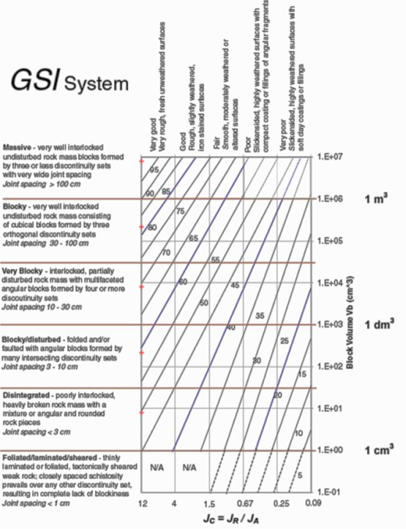
Quantitative Geological Strength Index (GSI) chart (Cai et al. 2004)
In this study, a methodology based on discrete fracture network (DFN) modelling combined with stochastic simulation is proposed to characterise rock block size distribution for determination of the GSI.
Approach to quantify rock block volume in the GSI system
Rock mass characterisation involves the establishment of a geometric model of the rock mass, including its discontinuity network. In conventional geomechanical mapping of rock masses, the measurement of the discontinuity geometries commonly requires physical contact in order to determine orientation, persistence, spacing, and condition. Rock block size, which is determined from the joint orientation, spacing, the number of joint sets, and persistence, is an important indicator of rock mass quality. Block size is an areal or volumetric expression of joint density.
Cai et al. (2004) assume that the joint sets are persistent and that the block area in 2D, Ab and the block volume in 3D, Vb can simply be calculated as
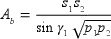
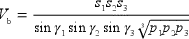
Illustration of block areas a and volumes b
Kim, Cai, Kaiser and Yang (2007) suggested that the block size in 2D and 3D for the rock mass with a non-persistent joint system can be realised by the distinct element code.
Figure 3a shows the blocks delineated by two non-persistent joint sets and Fig. 3b presents another example showing the blocks delineated by one continuous joint set and two discontinuous joint sets. At the moment, the distribution of the generated blocks follows a lognormal distribution, which is in agreement with the observation by Mahtab and Grasso (1992) and others that the probability density function of the block size and the joint persistence show a lognormal distribution.
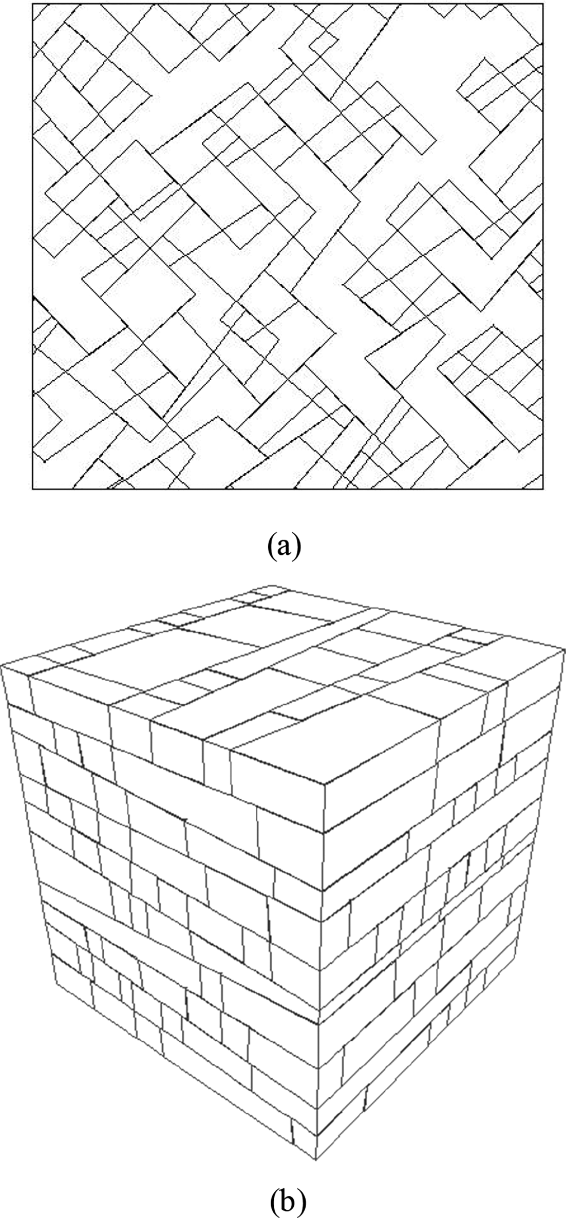
Example of the block system generated by discontinuous joint sets in 2D a and 3D b (Kim et al. 2007)
Although these methodologies can provide quantitative information on block volume for the GSI estimation, there is a fundamental limitation when applied to a complicated rock block system containing more than three joint sets and many random joints. In the next section, methodologies to prepare borehole based input data and realise rock block systems by DFNs for the estimation of the block volume distribution are introduced and discussed.
Estimation of a rock block system by discrete fracture networks
Different techniques exist to define an in situ block size distribution (Da Gama 1977; Hudson and Priest 1979; Maerz and Germain 1996; Rogers, Kennard, Dershowitz and Van As 2007). Some of the earlier studies could take into account one or more of the following: (1) having three or more discontinuity sets; (2) having non-persistent discontinuities; or (3) complex polyhedral shapes (Elmouttie and Poropat 2012).
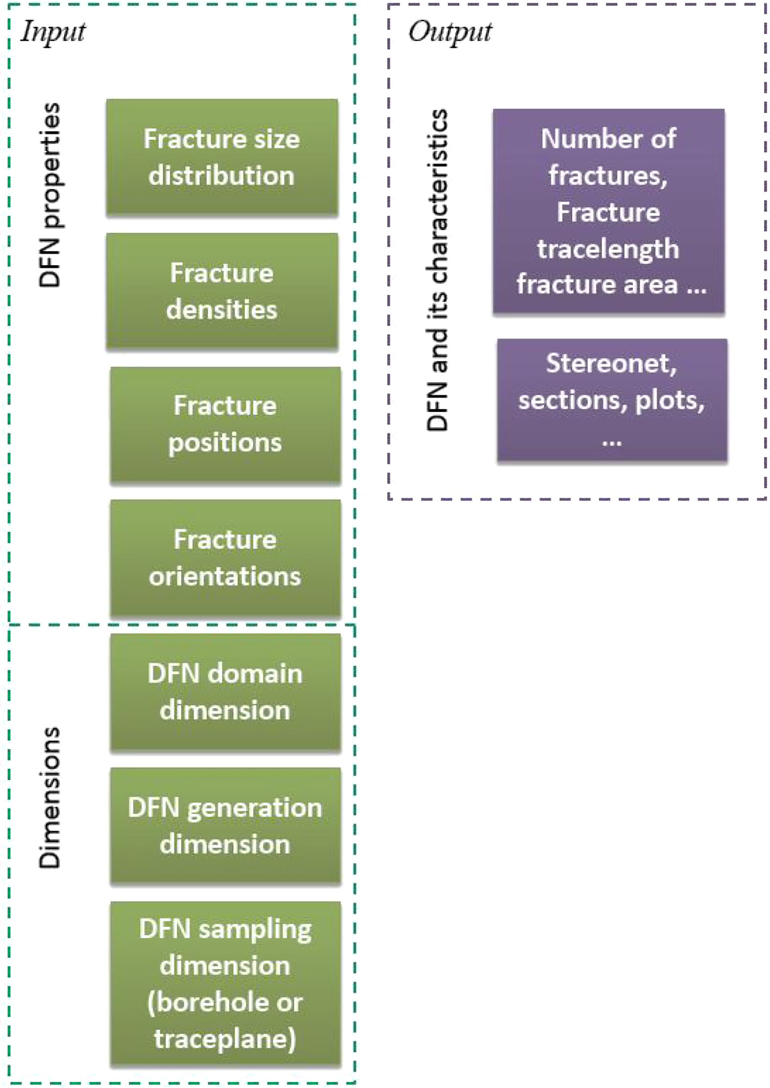
In this study, DFN models were created using field joint orientation data through statistical descriptions of joints. A set of statistical parameters were defined and joints were generated based on the statistical input, as well as real fracture orientation data from logged boreholes. As it is possible for any number of DFN realisations to satisfy the statistical criteria imposed, multiple DFN realisations were created for each unit. The overall information flow for this work is shown in Fig. 4.
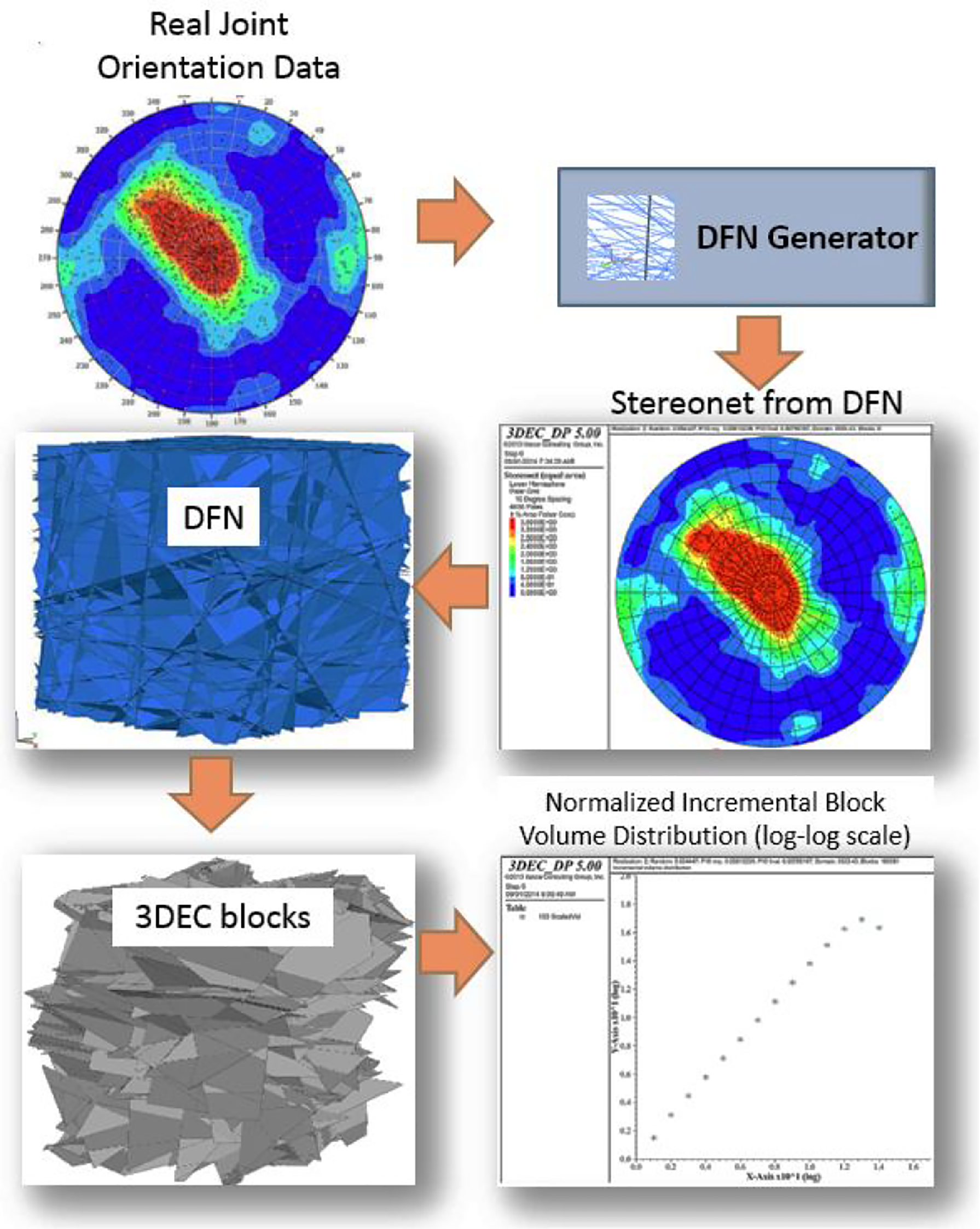
Analysis information flow
The real joint orientation data were obtained from acoustic televiewer (ATV) logs, and the DFN calibration data were obtained from fracture counts recorded during core logging.
The following methodology was used to create DFN block models:
A weighted joint orientation dataset from ATV logs was prepared. Cumulative fracture frequency distributions for calibrating each DFN was computed from core logged fracture counts. Discrete fracture network was created from real joint orientation data. Fracture generation and sample domain were defined, a virtual borehole was inserted in the model, and then, fractures were randomly added to the DFN until the target fracture frequency was achieved for the randomly selected percentile value and orientation group. Hundred DFN realisations were generated for each case. 3DEC models based on DFN realisations were created and block volumes were extracted. A normalised incremental block volume distribution was determined for each DFN realisation. The normalised block volume distributions from each realisation were combined to produce final distributions.
A detailed description of input data preparation and analysis is described in the following sections.
Preparation of input data for rock block volume estimation
Core logging and ATV data were combined for use as DFN input parameters to estimate block volume distributions for different structural domains. Bias corrections of the input data were required, specifically for ATV joint orientation data and fracture frequency data from core logging. In addition to the bias corrections, several fracture frequency cumulative distribution curves were developed for the DFN calibration process.
Joint sets that are perpendicular or near-perpendicular to the orientation of a borehole are preferentially sampled, whereas joint sets that are oriented in approximately the same direction as the orientation of a borehole will be under sampled (Terzaghi 1965). This leads to a bias in the joint orientation dataset that can be corrected using the Terzaghi weighting factor. However, a cutoff must be applied for joints that are oriented with small angles relative to the borehole orientation. This cutoff is required because as shown in Fig. 5, as the angle between the joint and borehole tends toward zero, the Terzaghi weighting factor tends towards infinity. Thus, application of the weighting factor to joints at small angles likely will result in several erroneous values. Ultimately, a cutoff limit of 15° was chosen.
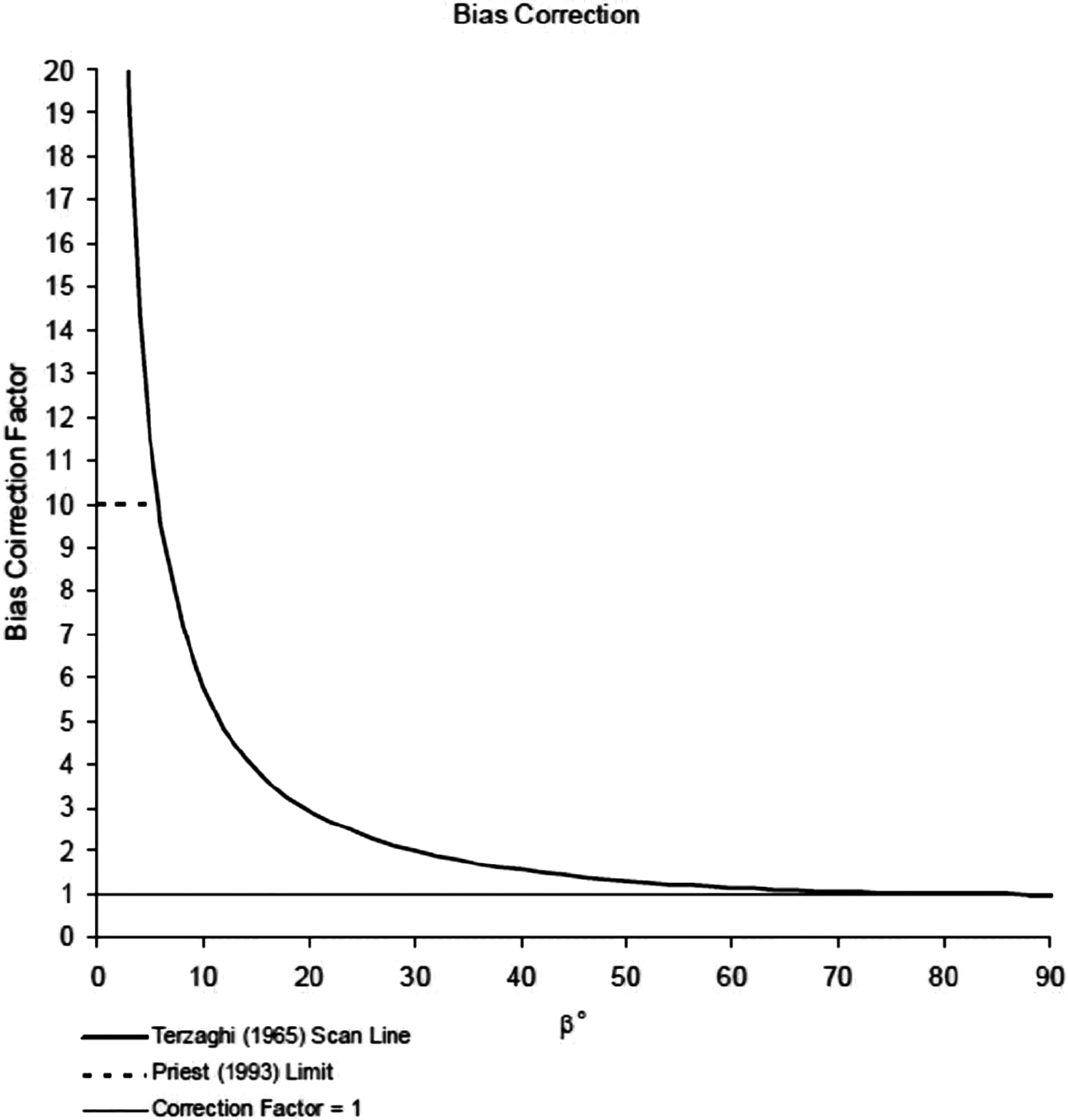
Relationship between the minimum joint–borehole angle and the Terzaghi weighting factor (Terzaghi 1965)
Borehole orientations for this study were predominantly NW trending with a plunge ∼75°. Therefore, by applying the 15° cutoff limit, joint sets that were trending parallel to this predominant borehole orientation would be under sampled. So, a second weighting factor was determined based on the number of boreholes with similar orientations. The binning for borehole counts was by quadrant, and the borehole orientation weighting factors were calculated for the boreholes in each bin. Then, these weighting factors were normalised so that they could be combined with the Terzaghi weighting factors to produce a single weighting factor for each logged joint.
Using the joint count data available from core logging records, a fracture frequency was determined for each 3 m (10 ft) of logged borehole length. A fracture frequency bias analysis was conducted so that any joint over-count bias (i.e., mechanically induced fractures logged as natural fractures) could be accounted for. The bias analysis included the following assumptions.
Depth measurements are more or less consistent between different techniques of core logging. Because ATV logging takes images of the intact borehole wall, it provides an excellent means of counting in situ fractures without over counting because of induced breakage caused by coring, extraction, transportation, and handling. Therefore, ATV fracture frequency is the benchmark. Fracture frequency distribution is approximately lognormal.
The bias correction consisted of transforming the core logged fracture frequency and ATV fracture frequency datasets to log–log scale (Fig. 6a) and performing an initial bias correction. The initial bias correction involved translating and scaling the fracture frequency data an appropriate amount such that the linear relationship between the two datasets had a slope of one and intercept of zero (Fig. 6b). This initial bias correction increases some of the data and reduces other data below a threshold value observed in the ATV dataset (i.e. 0.008 fractures per meter or a maximum joint spacing of 125 m). Therefore, a two-part final bias correction is performed where: (1) all data that were increased during the initial correction is reduced to its original value; and (2) all data that were reduced below the threshold value during the initial correction is increased to the threshold value (Fig. 6c). Finally, the data are converted from log scale back to normal scale (Fig. 6d).
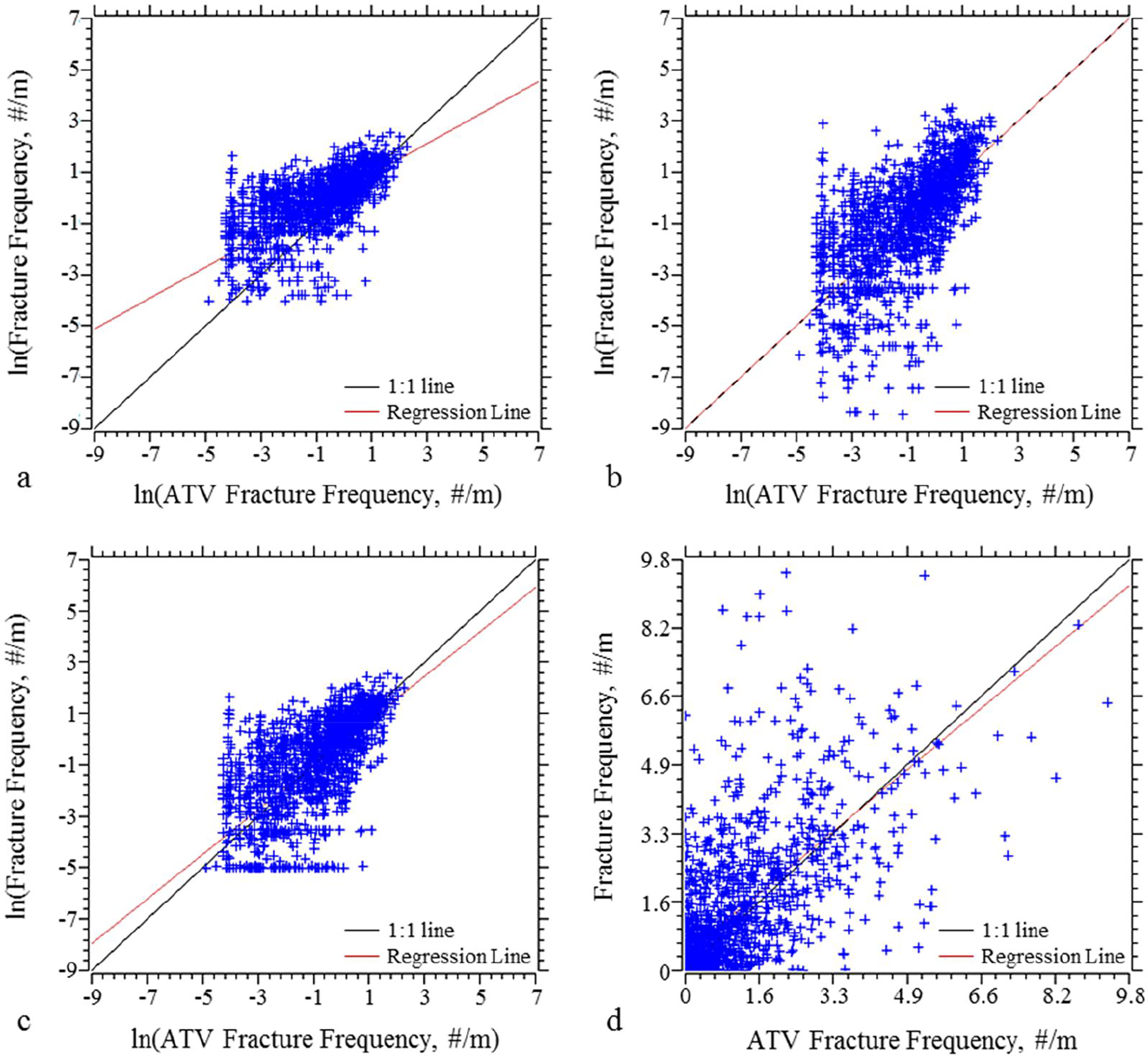
Fracture frequency bias correction process. Log–log plot of core logged versus acoustic televiewer (ATV) fracture frequency data a, log–log plot of initial bias correction of core logged data b, log–log plot of final bias correction of core logged data c, and normal scale plot of final bias correction of core logged versus ATV fracture frequency data d
A borehole's orientation will result in a preferential sampling of discontinuities perpendicular to the borehole axis, which is typically corrected using Terzaghi weighting. However, if a large percentage of boreholes exhibit a particular orientation parallel to the dip direction and dip of a major discontinuity set, then this discontinuity set will be under sampled, regardless of Terzaghi weighting. In order to account for potential under sampling of critical discontinuities, cumulative fracture frequency distributions were assembled for nine different orientation groups based on average borehole trend and plunge. The orientation of each group is shown in Fig. 7, where the first eight groups (31–38) cover boreholes plunging at angles less than 78°, and group 39 covers boreholes plunging at angles greater than 78°.
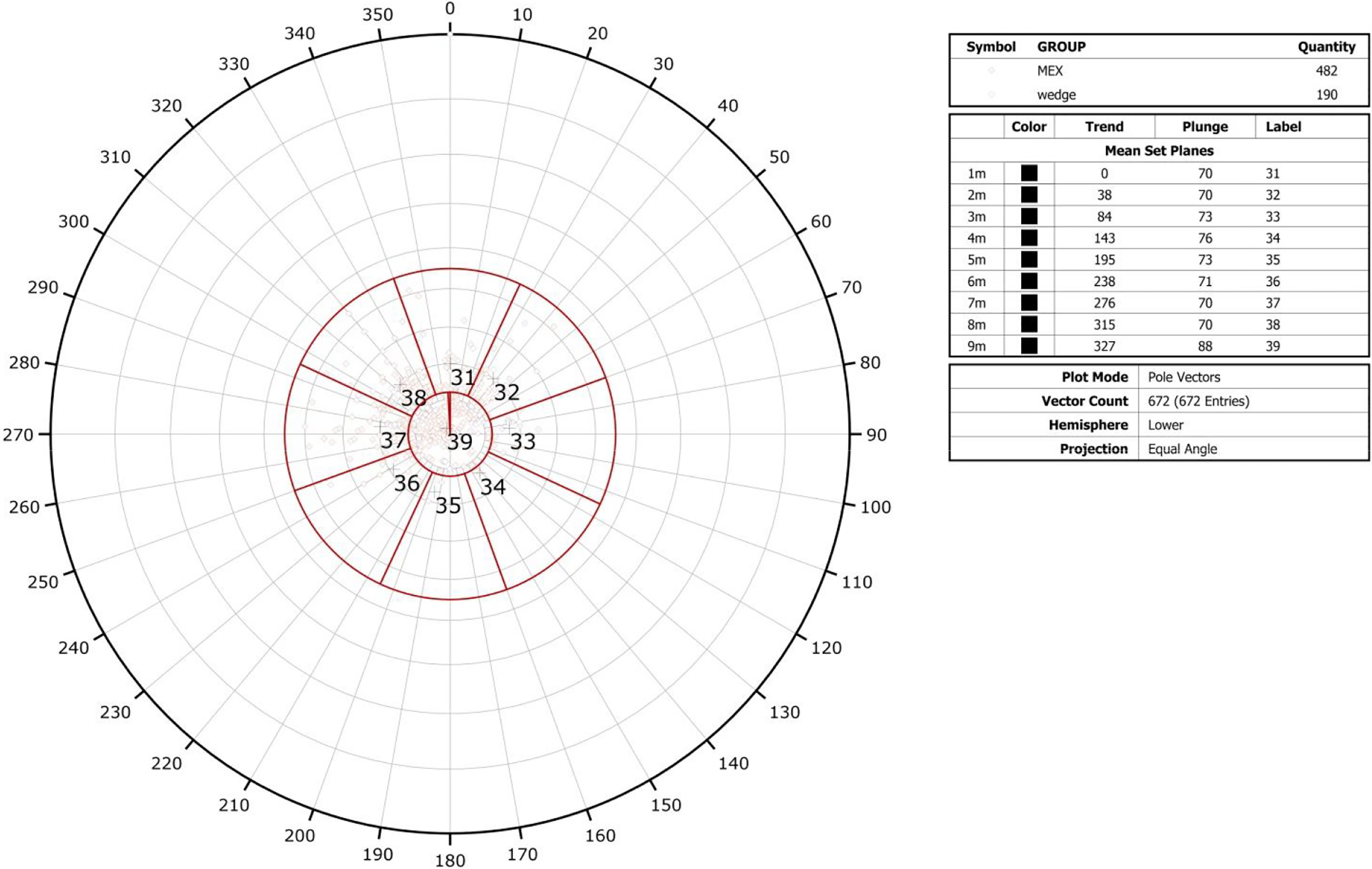
Fracture frequency borehole orientation groups
Mean trend and plunge were computed from the boreholes in each orientation group. Then, the mean trend and plunge values were used to construct virtual boreholes in the DFN and used to calibrate fracture density.
Then, cumulative distribution plots of fracture frequency were developed from the bias corrected dataset for eight different orientation groups of borehole. Figure 8 presents an example of the cumulative distribution curves from data used for DFN calibration. The domain # presents the geotechnical specific domain of the site.
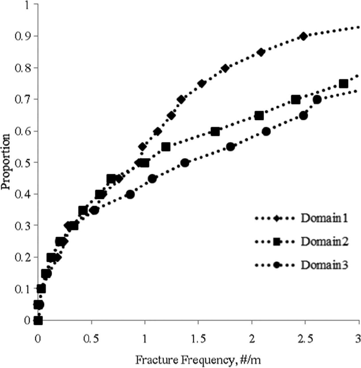
Example of cumulative fracture frequency distribution
Realisation of rock block system using 3DEC
A DFN generation module developed for Itasca software and 3DEC (Itasca Consulting Group Inc 2013) was used in this study. The DFN module generates a fracture population as a set of discrete, planar fractures of finite size. The geometrical characteristics of fractures are the fracture size (diameter), orientation and position distributions. In addition to the geometrical characteristics, the DFN module also supports fracture density as an input property. The schematic of the DFN logic is shown in Fig. 9.
Workflow in discrete fracture network (DFN) module
Two different domains with different sizes were defined for each DFN: a sample (observation) domain and a larger generation domain. The generation domain was always twice as large as the sample domain. In order to reduce finite-size effects, fracture positions were generated randomly within the generation domain. Fractures were made sufficiently large to be fully persistent through the sample domain regardless of where the feature existed in the generation domain. In order to produce representative block size distributions, the domain size in this work was adjusted for each fracture frequency value such that 45 fractures were formed along a virtual borehole extending through the domain.
The fracture frequency distributions produced for the domains during input data preparation were used to calibrate each DFN. For each domain, multiple realisations were performed choosing a random calibration fracture frequency each time.
A virtual borehole was generated and used as a density identifier during the DFN generation process to calibrate the model to a randomly selected fracture frequency. The borehole was created using appropriate fracture frequency distribution dip and dip direction angles.
Fracture orientations were bootstrapped to the field-collected values of fracture pole orientations (dip and dip direction). A fracture weighting factor was used to compensate for orientation bias because of sampling of a 3D DFN along a 1D borehole or scanline. During generation, the fracture orientations were selected randomly, i.e. bootstrapped from actual field data, while respecting the relative proportions based on the fracture weighting. Uniform random fracture positions were then chosen. The bootstrapping process continued until a target fracture frequency was reached along a virtual borehole. Once the target fracture frequency was achieved, the bootstrapping process ended and the DFN model was generated.
After the DFNs were generated, the resulting fracture frequency was calculated based on the count of the fractures that intersected the borehole. Examples of generated DFNs are shown in Fig. 10.
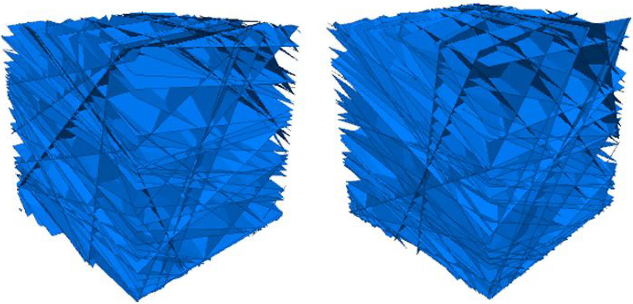
Examples for two discrete fracture networks (DFNs) realisations
3DEC models then were created using generated DFNs. First, a single block was generated and then it was divided into blocks based on the DFNs geometry. Next, all boundary blocks were identified and removed from the list of blocks (Fig. 11). A normalised block volume distribution was the final result of the rock block system generation.
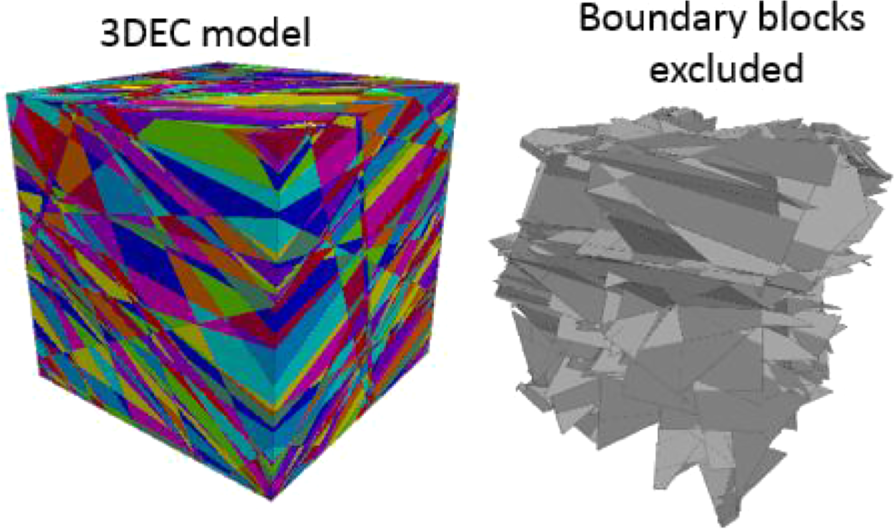
Example of a 3DEC model
Stochastic approach to determine GSI based on DFNS
A stochastic approach was used to estimate the rock mass strength. Monte Carlo simulations were used to obtain statistical distributions of tensile, uniaxial and confined rock mass strength based on the Hoek–Brown strength criterion using the available geotechnical data.
Figure 12 summarizes the path used to evaluate the distribution of Hoek–Brown parameters using the DFN-derived block volumes, geotechnical core logging and strength testing data.
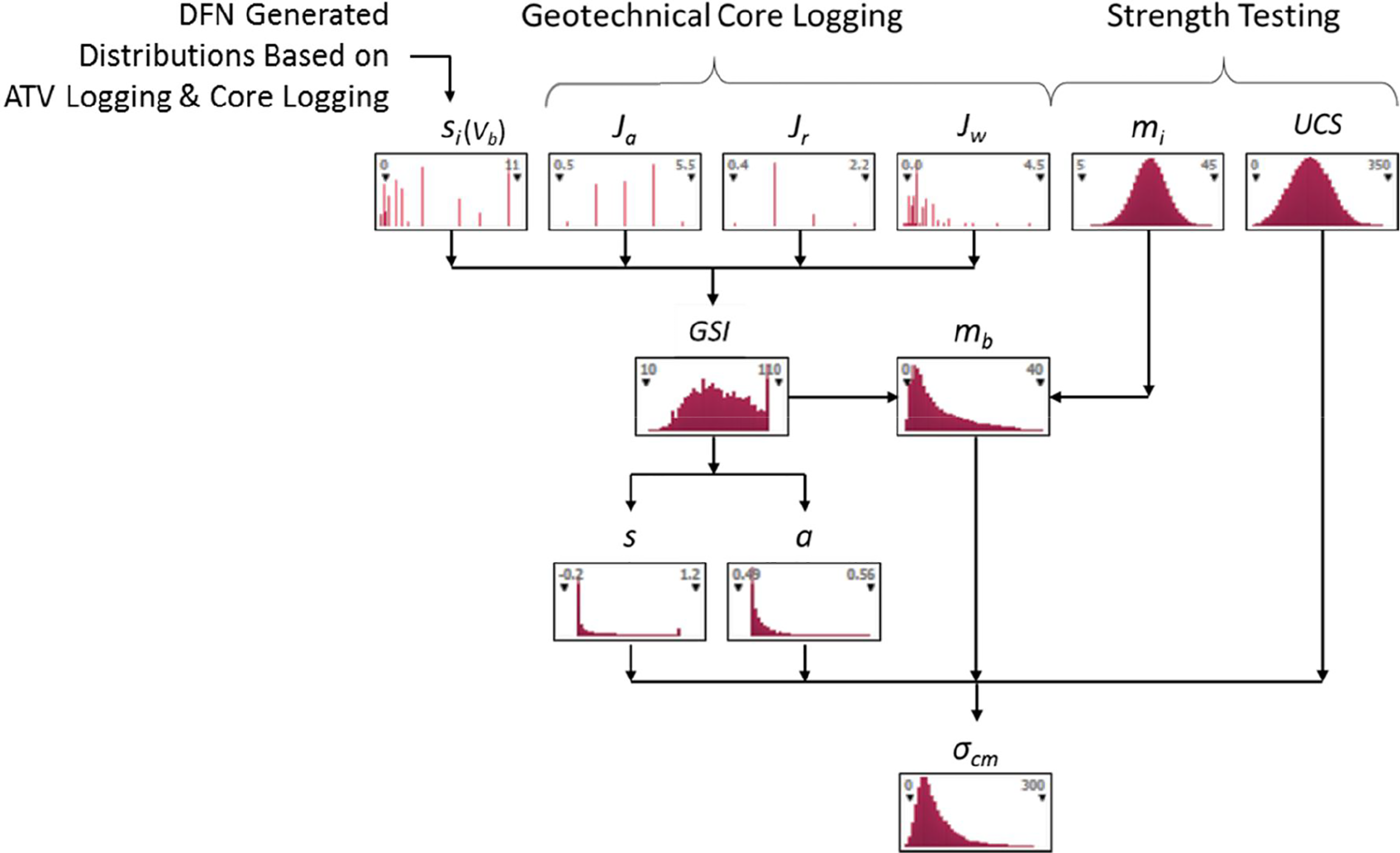
Monte Carlo procedure for estimating rock mass strength based on core logging and intact rock strength testing
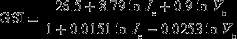
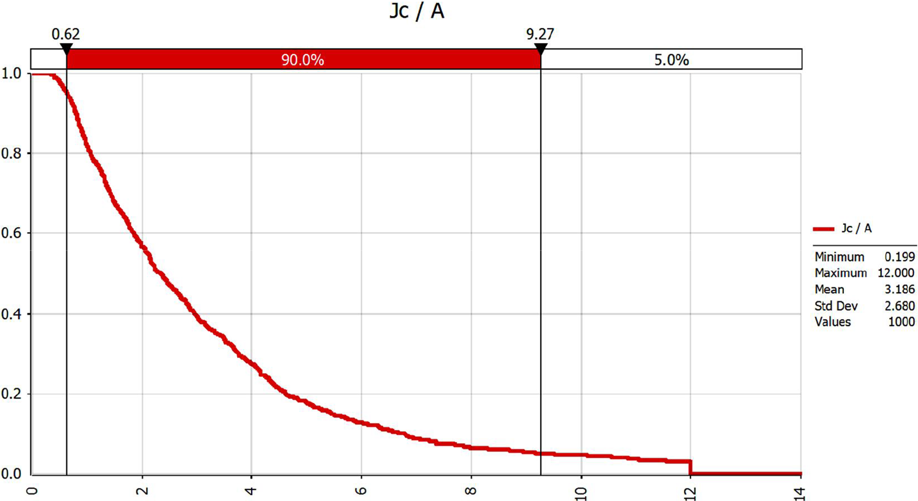
In order to quantify the original descriptive approach of estimating the GSI, the calibrated approach of Cai and Kaiser (2006) was used. As shown in equation (3), this approach incorporates calculated measures of block volume (Vb) and joint condition factor (Jc)
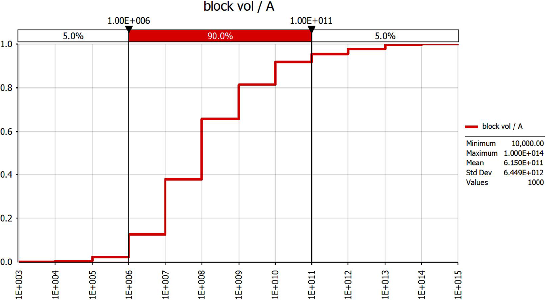
Example of probability distribution of rock blocks volume estimated by discrete fracture networks (DFNs)
Example of probability distribution of joint conditions used for Geological Strength Index (GSI) estimation
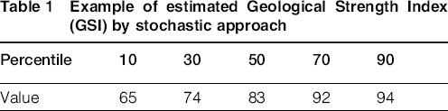
Example of estimated Geological Strength Index (GSI) by stochastic approach
Concluding remarks
The GSI system is the toolbox directly linked to engineering design parameters such as the Mohr–Coulomb or Hoek–Brown strength parameters or the rock mass modulus. Even though many pre-existing methodologies can provide quantitative information on block volumes for the GSI estimation, there is a fundamental limitation in complicated rock block systems. In this study, a DFN model incorporated with stochastic simulation was applied to characterise rock block size distribution for the determination of the GSI. The fracture frequency obtained from the core logging data was analysed and provided to the DFN model as input data. Realisation of the DFN and its verification were conducted to establish the joint systems corresponding to the fracture frequency observed during core logging. As a consequence, the results of the DFN simulations provided rock block size distributions used to successfully determine GSI distributions for various domains.
Acknowledgements
The authors would like to acknowledge the valuable discussions by Professors Davide Elmo and Doug Stead. This paper was originally presented at the first International Conference on Discrete Fracture Network Engineering (DFNE 2014) (19–22 October 2014, Vancouver, BC, Canada) and has subsequently been revised and extended before consideration by Mining Technology.