Rapid characterisation of fracture network realisations for hydrogeological,slope stability and geomechanical modelling

Abstract

For fractured rock masses, Monte Carlo simulation can be used to generate a multitude of fracture network realisations to support the estimation of the uncertainties in the fracture network properties and behaviour. However, the approach is limited by the computation time associated with performing fluid flow, slope stability or geomechanical analysis on each realisation, where it is often only feasible to analyse a small subset of these. The work presented in this paper facilitates the selection of fracture network realisations, representing conservative and aggressive scenarios, by using fast-to-compute geometry-based metrics. For hydrogeological analyses, we find that the success of such metrics depends on the complexity of the fracture network and we present an analysis of multiple scenarios to demonstrate this. Finally, we propose a similar approach for slope stability analyses and rock mass strength characterisation.

Keywords

Discrete fracture networks Geothermal reservoir characterisation Open cut mine slope stability

This paper is part of a special issue on Discrete Fracture Network Engineering (DFNE)

Introduction

Current rock mass engineering relies heavily on numerical modelling, which allows the representation of complex physics and large scales. Numerical modelling has become an essential requirement for almost all fields of rock mass engineering including slope stability, reservoir characterisation, blasting and rock processing. Heterogeneity and anisotropy of rock mass properties must be captured in the modelling process. Owing to the limited understanding of geology, hydrogeology, discontinuities and the rock matrix in the field, two types of uncertainty are present, namely, model and stochastic uncertainty. The latter exists even if our understanding is accurate because the properties of interest (e.g. rock mass strength, fracture diameter, permeability) must be treated as stochastic variables.

As computing power increases in capability and affordability, the ability to more accurately model the rock mass has also improved. Coupled physical processes, complex geologies and stochastic processes can all be numerically simulated. Nonetheless, the computing resources are finite and decisions still need to be made by the practitioner on which aspects of the problem to represent numerically. Representation of the aforementioned uncertainties in this modelling process is often neglected in an attempt to model the most sophisticated physics and detailed geometry possible (Fig. 1). There are perhaps several reasons why this aspect is often neglected, ranging from the desire of physical scientists to focus more on ‘interesting physics’, the aesthetics associated with the capabilities of modern day computer visualisations to represent large scale problems, and the esoteric nature of uncertainty quantification.

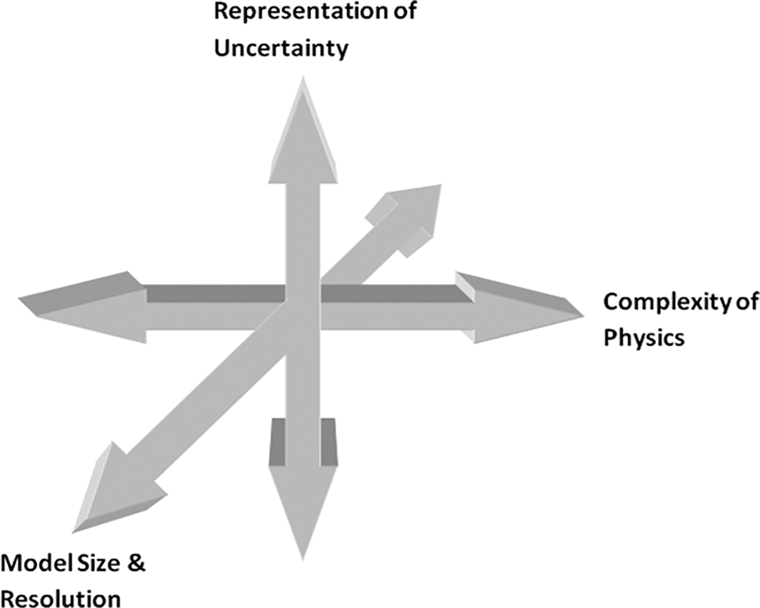
The parameters associated with the modelling process

For practitioners wanting to perform uncertainty quantification, there are two fundamentally different approaches to model the heterogeneity in the rock mass properties. These can be labelled stochastic continuum methods, consistent with equivalent porous medium (EPM) approaches, and stochastic discrete methods using discrete fracture networks (DFNs). Each has its advantages but DFN modelling is particularly suited to scenarios where the spatial heterogeneity in the fracture network properties is critical to the modelling of the process being investigated. For understanding fluid flow through a given fracture network cluster (group of connected fractures), only a subset of the cluster [known as the backbone (Odling et al. 1999)] may be responsible for the conduction through fractures. If this hierarchy cannot be represented with sufficient fidelity using EPM, then a DFN approach is warranted (Fig. 2).

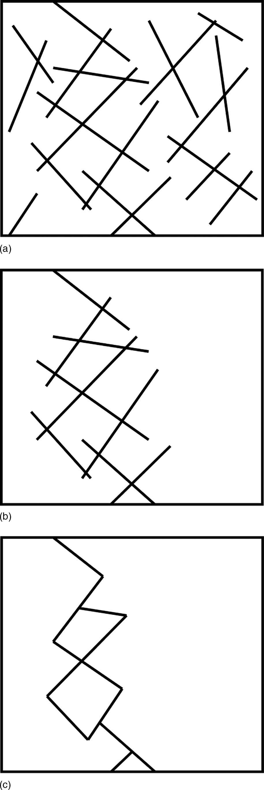
A fracture network a, percolating cluster b and backbone c in two-dimensional space

Explicit representation of fractures and rock mass defects is fundamental to DFN modelling and this imposes significant computational costs (processing time and memory consumption). Stochastic modelling may involve generation and accompanying analysis of hundreds or thousands of equiprobable, but potentially very different DFN realisations to determine confidence intervals for model predictions (such as in Monte Carlo simulation). In practice, the computer codes capable of modelling the complex physics across large scales associated with geomechanical and hydro-geomechanical processes are so computationally expensive that modelling is typically limited to only a small selection of DFN realisations. The work reported here provides guidance to allow accurate characterisation of the confidence intervals by identifying which DFN realisations should be selected for modelling. By doing so, the number of numerical simulations can be drastically reduced.

Discrete fracture network models used for solving flow and transport equations in three-dimensional networks require some form of a discretisation scheme. The discussion in Jing (2003) provides a good review of the discretisation schemes used to model fluid flow in three-dimensional fracture network models. The simple pipe model represents a fracture as a pipe of equivalent hydraulic conductivity starting at the disc centre and ending at the intersections with other fractures, based on the fracture transmissivity, size and shape distributions (Cacas, Ledoux, De Marsily and Tillie 1990).

Traditionally, reservoir modelling of fractured rock masses is based on the EPM approach but implements what is known as a dual-porosity model (dual referring to the fracture network vs the rock matrix). This modelling is valid for rock masses with high-fracture frequencies and well-connected networks so that the fracture properties can be averaged over a grid block. Clearly, this approach is of limited use for reservoirs where the flow occurs predominantly through a small number of fractures in the network and the DFN approach is therefore justified.

The stability of a slope composed of a fractured rock mass can also be modelled using the DFN approach and either discrete element or hybrid continuum/discontinuum methods are typically used. The DFN approach can enable structurally controlled failures to be explicitly analysed. This is particularly important in open pit mining where the frequency of inter-bench and bench-scale failures must be quantified as their influence on safety and operations on mines can be significant.

Rock mass strength is recognised to be influenced by the strength of intact rock, joint density and orientation and the joint mechanical properties. The most widely used empirical methods for scaling rock strength [known as Hoek–Brown criteria (Hoek and Brown 1980; Hoek and Brown 1997)] and the joint properties of the rock mass, are captured by the geological strength index (GSI) classification of the rock mass (Hoek, Marinos and Benissi 1998; Marinos and Hoek 2000). In this scheme, joints are represented as points on a 2D chart where the X axis represents the defect in mechanical properties, while the Y axis reflects jointing intensity.

One of the attractive practical benefits of DFN modelling is the ability to remove or reduce the subjectivity of characterisation of joint intensity within a rock mass. However, when a DFN realisation is developed, whether from a deterministic or stochastic (or both) realisation of jointing, the resultant rock mass description can be characterised with certainty by metrics to a degree that is not possible from direct field mapping. The attributes of the DFN can then be directly sampled in an analogous approach to field mapping, allowing the underlying stochastic joint properties to be adjusted if needed.

The objective of this work was to investigate the efficacy of using geometry based, fast-to-compute metrics for characterisation of fracture network realisations. One of the main goals in probabilistic analysis is uncertainty quantification and therefore metrics are sought for selection of realisations that lead to vastly different outcomes in DFN fluid flow modelling and stability analysis. For DFN generation, the Siromodel software developed by CSIRO as part of the large open pit (LOP) project (Read and Stacey 2009) was used. This software provides facilities for Monte Carlo simulation of DFN realisations and the subsequent polyhedral model and stability analysis for open pit slopes.

Authors have assessed the metric validity using a numerical code, namely, Itasca's Slope Model software (Slope Model User's manual, Itasca Consulting Group 0000), which incorporates a lattice node generator for the mechanical modelling (Cundall 2008) and a pipe network generator for the fracture flow component. This software was also developed as part of the LOP project (Read and Stacey 2009) for the simulation of hydro-mechanical processes for slope stability analyses in deep open pit mines. This code utilises the synthetic rock mass [SRM (Pierce, Cundall, Potyondy and Mas Ivars 2007; Mas Ivars et al. 2011; Mas Ivars, Deisman, Pierce and Fairhurst 2007)] approach based on the distinct element method. Typically, SRM models have used the bonded particle approach to model the intact rock matrix and a smooth joint model (SJM) to allow slip and separation at particle contacts on fracture surfaces. Much greater efficiency can be realised for brittle rock if a ‘lattice’ consisting of point masses (nodes) connected by springs replaces the balls and contacts (respectively). Fluid flow throughout the joint network and the rock matrix also is modelled, with the resulting pressures being used to compute effective stresses (hence, failure conditions) on each joint element. The code is capable of modelling hydro-mechanical coupling (not utilised in this work) and fracture formation and propagation.

The scope of the work was constrained in several ways. In the hydrogeological studies, only fluid flow through the fracture network was modelled (i.e. rock matrix considered impermeable) and only pre-existing fracture geometries were considered, equivalent to a static production scenario of a geothermal reservoir or in situ fracture network in an excavated slope. This work also has applicability to DFN-based analysis of hydraulic fracturing (Pettit et al. 2011) where it has been shown that multiple DFN realisations are required for uncertainty quantification (Xu, Dowd and Mohais 2012). Fracture network geometries were limited to those sufficiently complex to demonstrate the efficacy of the metrics for realistic scenarios but simple enough to ensure reasonable simulation times. For the slope stability and geomechanical analyses, no fluid flow was considered. Although variance in fracture apertures can be analysed using the method described in this paper, for simplicity, all modelling presented assumes fracture apertures of 1 mm. No hydro-mechanical or thermal coupling physics were investigated.

Application to hydrogeological characterisation section of this paper presents a validation of the metrics being assessed using simple DFN geometries and Realistic scenarios section tests the most successful metrics against more realistic DFN geometries. Application to slope stability analyses section discusses the application of this methodology to slope stability and other geomechanical analyses.

Application to hydrogeological characterisation

Validation of proposed metrics

Several geometry-based metrics were considered for this work, namely, minimum intersection trace length per backbone; sum of intersection trace lengths per backbone; sum of backbone areas; flow solution using simple pipe network (referred to as ‘Qsum’). To extract the geometric properties of the individual DFN realisations and derive the metrics, custom software was written by the authors. The ‘minimum intersection trace length per backbone’ refers to determining the shortest intersection trace (i.e. potential ‘pinch point’) associated with a backbone. The ‘sum of intersection trace lengths per backbone’ refers to adding the lengths of all intersection traces associated with a backbone. Similarly, the ‘sum of backbone areas’ refers to adding the areas of each fracture associated with a backbone.

The metric, referred to as ‘Qsum’, proved to be the most successful, and is explained here in more detail.

Flow solution using simple pipe network – ‘Qsum’

The metrics being considered in this work all relate to the geometry (areas and lengths of intersecting traces) of the fractures associated with the percolating backbone. The pipe network generators described by other authors (Long, Gilmour and Witherspoon 1985; Cacas et al. 1990; Dershowitz and Fidelibus 1999) and available in third party codes often use this geometry to generate the equivalent pipe network properties (connectivity and pipe conductances). A significant computational cost is associated with solving for the flow patterns on each individual fracture based on the geometry of the intersection traces on that fracture. Authors have investigated that the significance of neglecting this aspect of the flow solution and simply solving for the flow assuming a constant head pressure at each fracture. Further, to keep computation times down, we have developed a simple pipe network generator, which utilises the intersection trace data (lengths and relative separation on a given fracture) to assign pipe conductances.

The equivalent pipe conductances are calculated assuming parallel plate theory with plate width being the average of the trace lengths and plate length given by the separation of the trace centroids. If a fracture was completely partitioned by a trace, the pipe network was constrained accordingly and no pipes were generated across that trace. This was implemented to approximate the flow scenario where such a persistent trace must affect the flow. This aspect of the algorithm essentially accounts for face topology. A normalisation factor was also determined to ensure that the sum of the pipe ‘areas’ did not exceed the area of the original fracture – such an anomaly would not be otherwise prevented because the trace connectivity does not fully respect the spatial locations of the traces on the fracture (or, more formally, flow within the fracture is not being solved for).

Once the pipe network has been generated, we assume that the flow Q along the pipe is driven by the head loss ΔP and that the flow is proportional to the conductance C of the fluid through the pipe, that is (1)

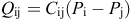
Moreover, we assume laminar flow and parallel plate flow, so that the conductance between two connected nodes denoted by i and j is given by: (2) where a, W and L represent the fracture aperture, width and length, respectively, and μ represents the dynamic viscosity of the fluid.

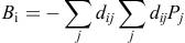
If there is conservation of mass at each node (i.e. no net gain/loss of fluid), then the pressure at node j can be expressed as the sum of the flows to/from its neighbours (3) (4) To simplify, the problem is reformulated so that the pressure at the central node is defined in terms of those at its neighbours as shown in Figure 3. The pressure at the central node is then determined by summing the weighted neighbour pressures normalised by the sum of the conductances. Authors also define a parameter d_ij, which represents the weighted conductances at the internal nodes.

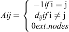
Authors then solve for the pressures at the internal nodes given the constraints at the boundary nodes using the following matrix formulation (5) where x represents the pressures P_i and A represents the symmetric, sparse matrix constructed for internal nodes with

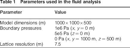
For external nodes, we construct the B matrix (6) Using this formulation, one can solve for the pressures at the internal nodes. Authors refer to this metric as ‘Qsum’. The DFN was then imported into the numerical code for fluid analysis and comparison with the metrics. The parameters used are shown in Table 1.

Table 1

Parameters used in the fluid analysis

Parameter	Value
Model dimensions (m)	1000 × 1000 × 500
Boundary pressures	1e6 Pa (x, y = 0 m)
	5e5 Pa (z = 0 m)
	0 Pa (x, y = 1000 m, z = 500 m)
Lattice resolution (m)	7.5

Validation DFN geometries

A number of simple DFN geometries were used to validate the metrics and compare their performances. Geometries were chosen for which analytical solutions could be derived including series and parallel flow networks. From these simulations, a number of decisions were made regarding the reliability of the flow solver for this work. A lattice resolution of 7.5 m over the domain volume of 0.5 × 10⁹m³ was chosen as a compromise between model resolution and computing requirements (Fig. 3).

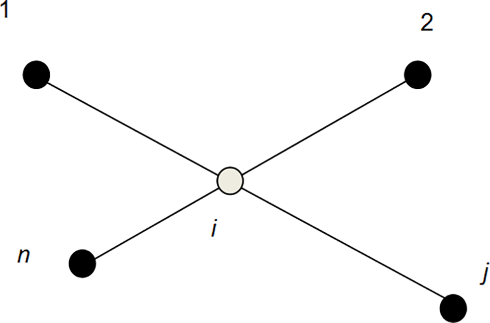
A representation of a simple network consisting of a node (white) connected to four nodes

The results are presented in Fig. 4. From the study of these metrics, it was observed that a metric based on the geometry of the DFN can be used to predict the relative permeabilities of simple DFN geometries at least in a qualitative sense. For realisations with geometries conducive to parallel flow, a metric based on a simplified solution of the flow equations (Qsum) shows the most promise and was selected for further analysis.

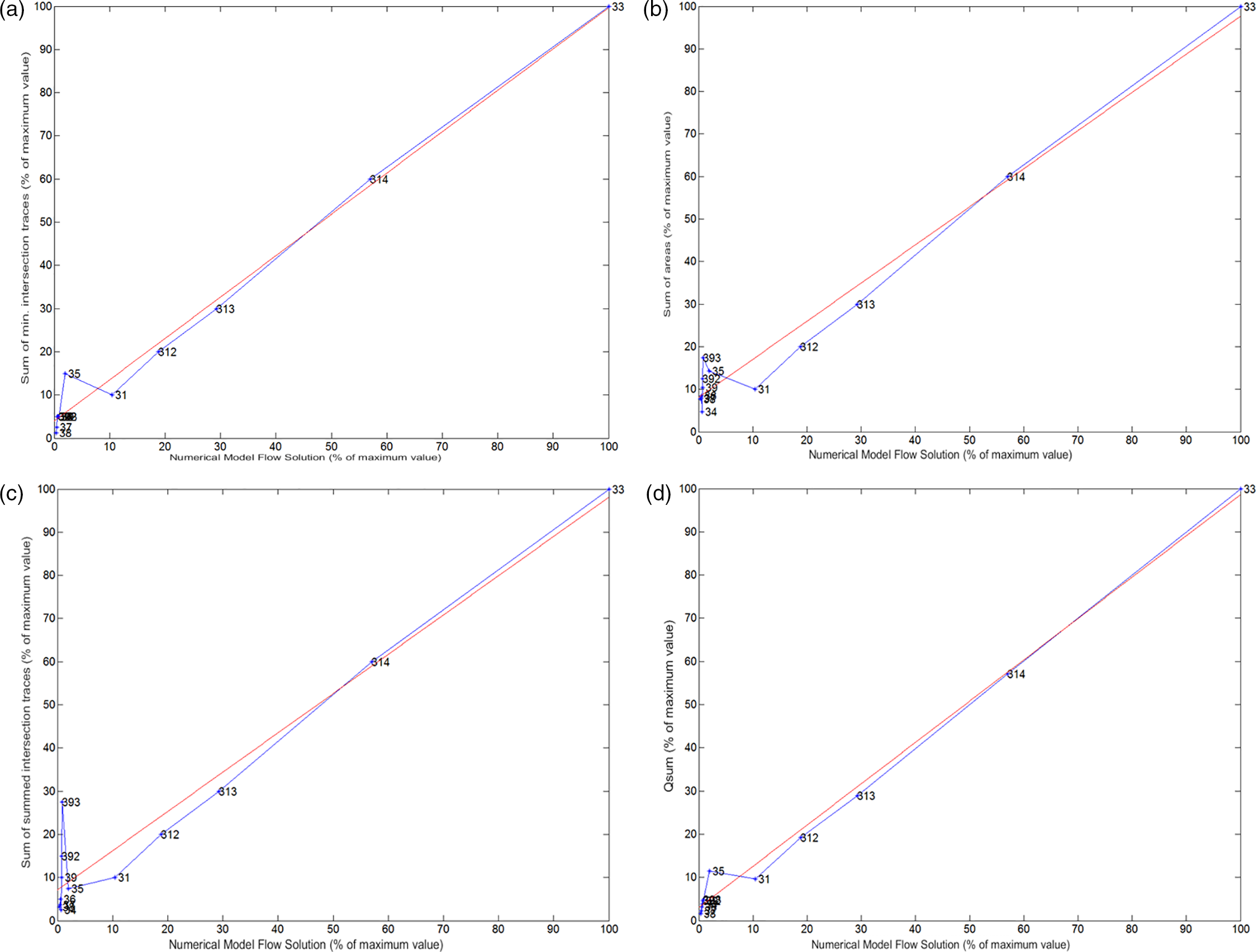
Metrics vs numerical code predictions of outflow. a Sum of minimum intersection traces for cluster backbones, b sum of backbone areas, c sum of intersection traces within backbones and d flow calculation based on simple pipe network shown. Linear trends are shown in red

Realistic scenarios

2.5D simulations

A series of increasingly realistic DFN geometries were used to investigate the performance of the Qsum metric against the predictions of the numerical code.

Some simulations were conducted using a constrained problem space to determine the applicability of the metrics confirmed in Application to hydrogeological characterisation section. A 2.5-dimensional (2.5D) approach was used to facilitate interpretation and fracture locations were constrained to a single plane (XZ) but with three-dimensional (3D) forms (i.e. polygons). Initially, three realisations were generated each with nine fractures (hexagons). The boundary fractures were 500 m wide, six of the fractures were 300 m wide but the central fracture in each realisation had a width of 300, 200 and 150 m, respectively. The third realisation is shown in Fig. 5 and represents the ‘touching’ or ‘pinch point’ case such that, from a geometrical point of view, no further decrease in fracture size would permit flow. Of course, given the finite lattice resolution used in the numerical code, the discretisation process would alter these characteristics.

The third of a series of three realisations of two orthogonal fractures sets

Figure 6 shows the relationship of the Qsum metric for each of the three simulations (referred to as 111, 222 and 333) to the numerical code predictions. Further, two simulations labelled 444 and 555 were also generated with minimum sized interior fractures and minimum sized interior and boundary fractures, respectively. Results for other simulations discussed in the next section are also shown. The correlation seen in the validation simulations described in Application to hydrogeological characterisation section is confirmed although some simulations suffer from lattice resolution effects.

Qsum metric versus Slope Model predictions for several of the realisations of two orthogonal fractures sets with randomly sized interior fractures. Simulation identifications are shown in red indicate the presence of intersection trace lengths below the recommended lattice resolution threshold. Linear trends are shown in red

The analysis was extended with all seven fractures within the bounding volume being assigned randomly generated sizes. A uniform distribution was used with limits of 150 m (i.e. the limiting case for connectivity) to 300 m. Using these parameters, 30 simulations were generated with a percolation probability of around 70%.

Figure 6 shows the results from this analysis for several of the realisations from the set of 30. Good correlation is evident between the Qsum metric and the numerical code predictions. The offset from the origin is presumed to be a result of the discretisation effect that is very apparent in the numerical code data. Note that some simulation identifications have been shown in red to indicate that at least one intersection trace lengths is below the recommended resolution threshold of the lattice/pipe network (roughly three to four lattice resolutions). These results were promising and encouraged investigation of more realistic DFN.

Another two realisations were generated to investigate the metrics’ ability to deal with parallel fluid flow paths within the context of the 2.5D simulations (see Fig. 7).

An example discrete fracture network (DFN) geometry used for the parallel flow path simulations

Numerical model flow solution

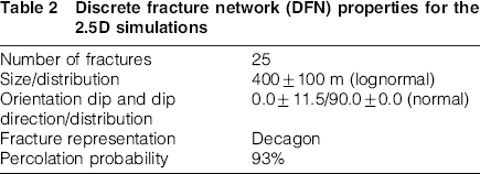
Finally, the analysis was further extended to use a more realistic DFN geometry with more closely packed, sub-horizontal fractures providing both series and parallel flow paths. Table 2 shows the DFN properties used for these simulations. Sub-horizontal fractures were generated to approximate the geometry of the full 3D simulations described in the next section.

Table 2

Discrete fracture network (DFN) properties for the 2.5D simulations

Number of fractures	25
Size/distribution	400 ± 100 m (lognormal)
Orientation dip and dip direction/distribution	0.0 ± 11.5/90.0 ± 0.0 (normal)
Fracture representation	Decagon
Percolation probability	93%

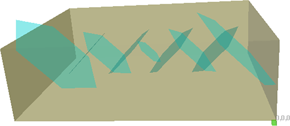
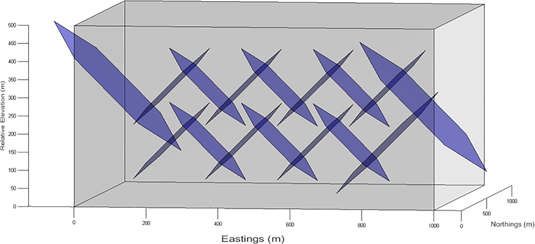
An example DFN realisation is shown in Fig. 8.

Example discrete fracture network (DFN) realisation from the 2.5D simulations

Figure 9 shows the distribution of Qsum flows for all 30 realisations. The use of sub-horizontal fractures added further sensitivity to the finite resolution of the lattice/pipe network used in the numerical code. This is a limitation of the current experimental method as it will prevent confirmation of the metric's validity for more realistic and dense fracture networks. Although some attempt has been made to identify the realisations that are incompatible with the lattice resolution, this has been limited to an analysis of intersection trace lengths. In general, other fracture network properties that require interrogation include fracture separation, fracture size (although not so relevant in these DFN realisations as the size distribution was constrained) and fracture proximity to the boundaries of the model.

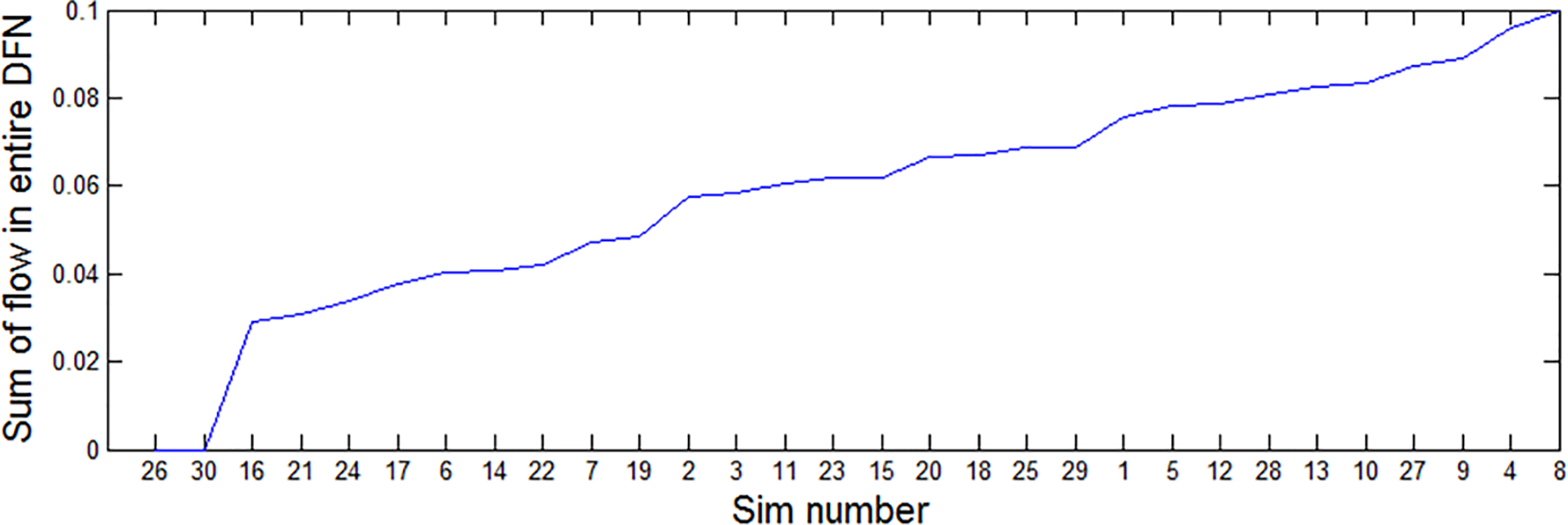
Distribution of Qsum flows using simple pipe networks for all 30 realisations

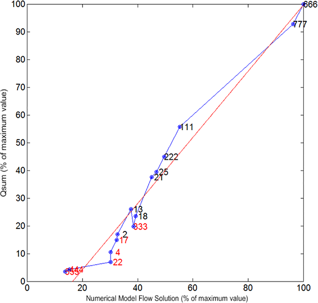
Owing to limited computational resources, a selection of 2.5D realisations representative of the various backbone areas and minimum trace lengths were used for the analysis. The results are shown in Fig. 10 and the Qsum metric performs reasonably well.

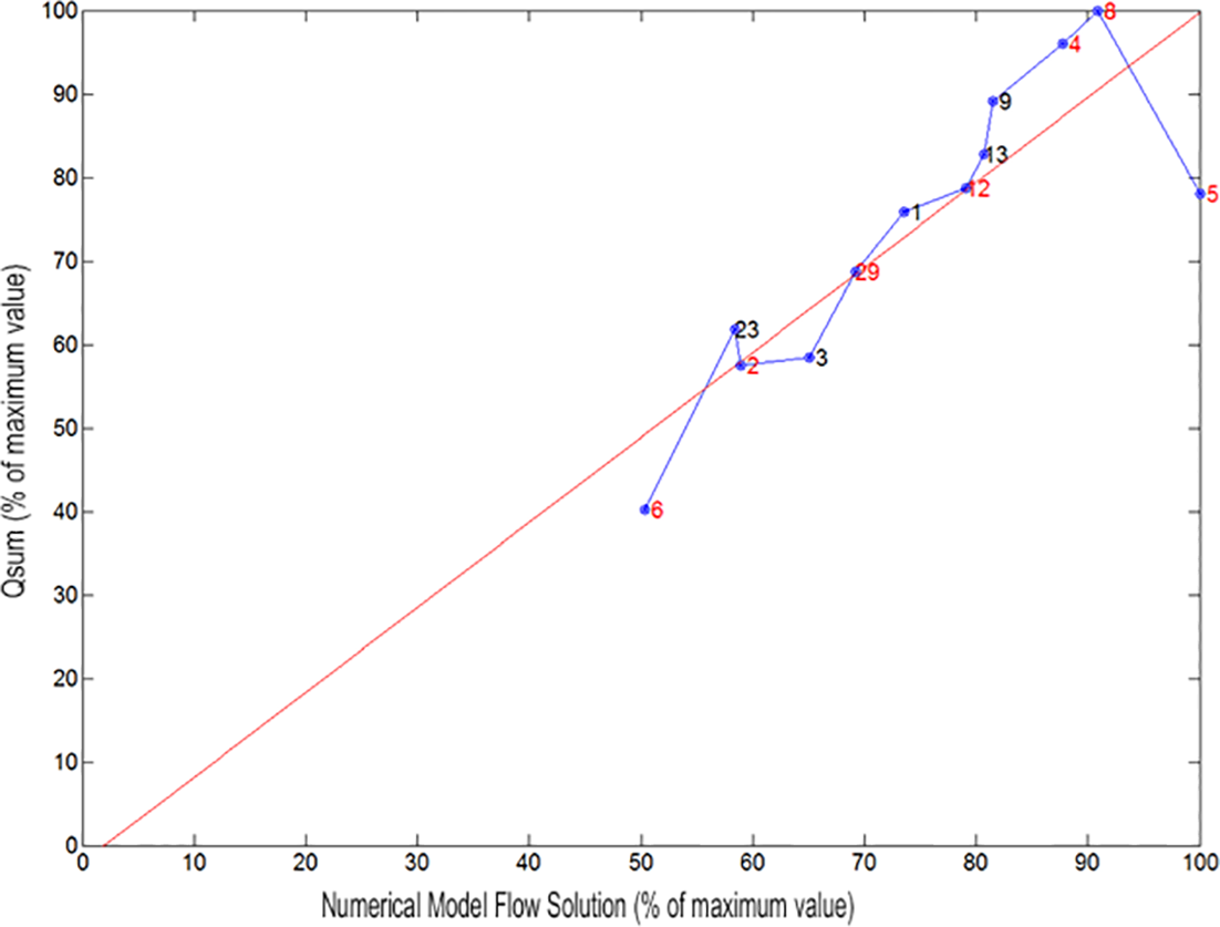
Qsum metric vs Slope Model predictions for the selected 2.5D realisations. Simulation identifications are shown in red indicate the presence of intersection trace lengths below the recommended lattice resolution threshold. Linear trend is shown in red

Full 3D simulations

Finally, and notwithstanding the limitations identified in the 2.5D simulations, analysis of DFN geometries that more accurately capture the heterogeneity in a geothermal reservoir was performed. Justification for the geometry chosen was based on literature describing fracture networks in DFN reservoirs consisting predominantly of sub-horizontal fractures in both pre- and post-stimulation phases (e.g. Xu et al. 2012). The choice of orientation and size parameters for the DFN generation was motivated primarily to achieve percolating clusters for flow analysis without the need to model fracture propagation. The properties are shown in Table 3.

Table 3

Properties for full 3D fracture flow simulations

Number of fractures	100
Size/distribution	400 ± 100 m (lognormal)
Orientation dip and dip direction/distribution	0.0/0.0 (fisher κ = 50)
Fracture representation	Decagon
Percolation probability	100%

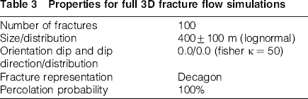
The pressure boundary conditions for these simulations were set for all three axes. The numerical code did not accommodate specification of gradients in boundary pressures and therefore incompatible conditions were present on three of the edges that join low- and high-pressure boundaries. After some trials, the number of fractures per realisation was set to 100 to ensure around 100% of realisations generated percolating backbones across at least two opposing domain boundaries.

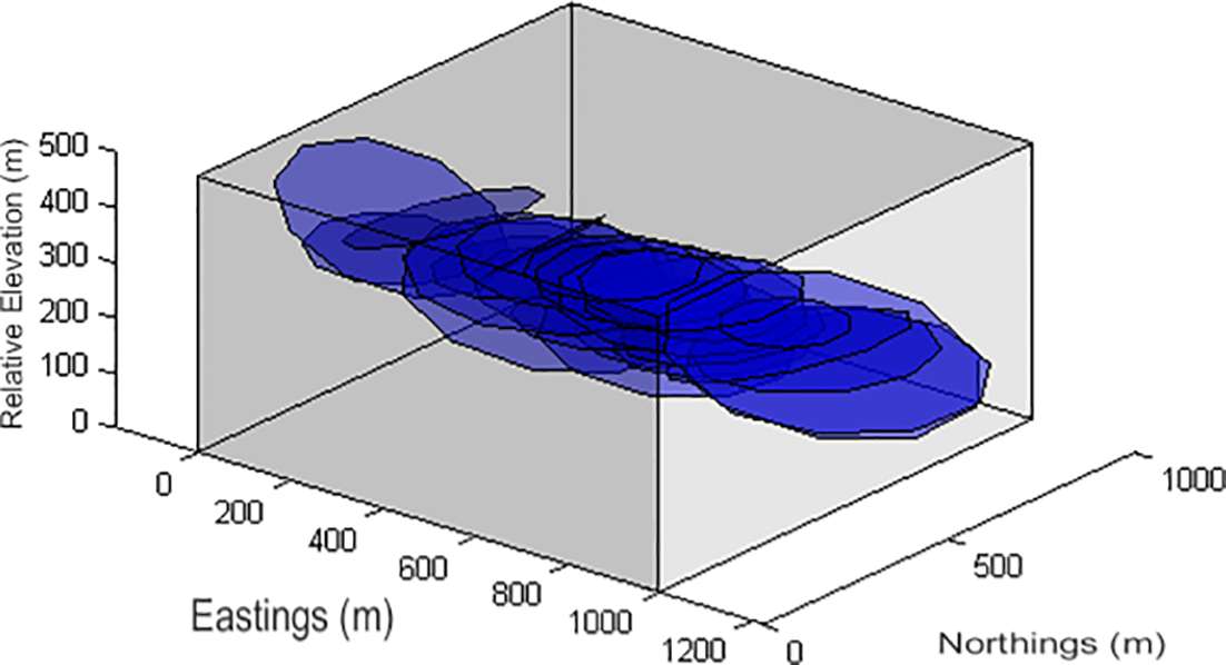
Figure 11 presents an example DFN realisation from this series of 30 realisations.

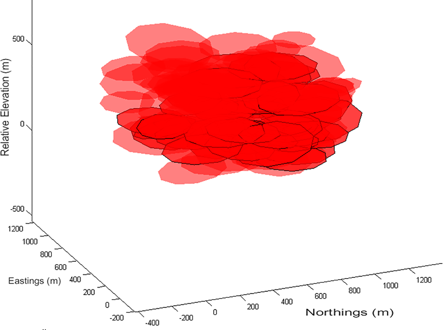
A discrete fracture network (DFN) realisation for the full 3D simulations with the backbone of one of the two spanning clusters identified (fractures with edges shown)

Owing to computational resource constraints, not all realisations could be simulated within the numerical code and a selection of realisations, which were reasonably representative of the various backbone areas and minimum trace lengths of all 30 realisations, were used. The results are shown in Fig. 12.

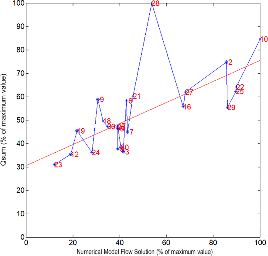
a Qsum metric vs numerical code predictions for the selected 3D realisations. Simulation identifications are shown in red indicate the presence of intersection trace lengths below the recommended lattice resolution threshold. Linear trends are shown in red

The level of the correspondence of the Qsum metric to the numerical code predictions for full 3D simulations is poor although the trend is still clear. Figure 13 shows visualisations of an example realisation and aside from a handful of fractures that bridge boundaries with incompatible pressures, the agreement is reasonable. Therefore, notwithstanding the poor correlations between the Qsum metric and the numerical code results seen for full 3D simulations, repeating the analysis using resources capable of both finer discretisation and more control over boundary conditions would be a promising avenue of research.

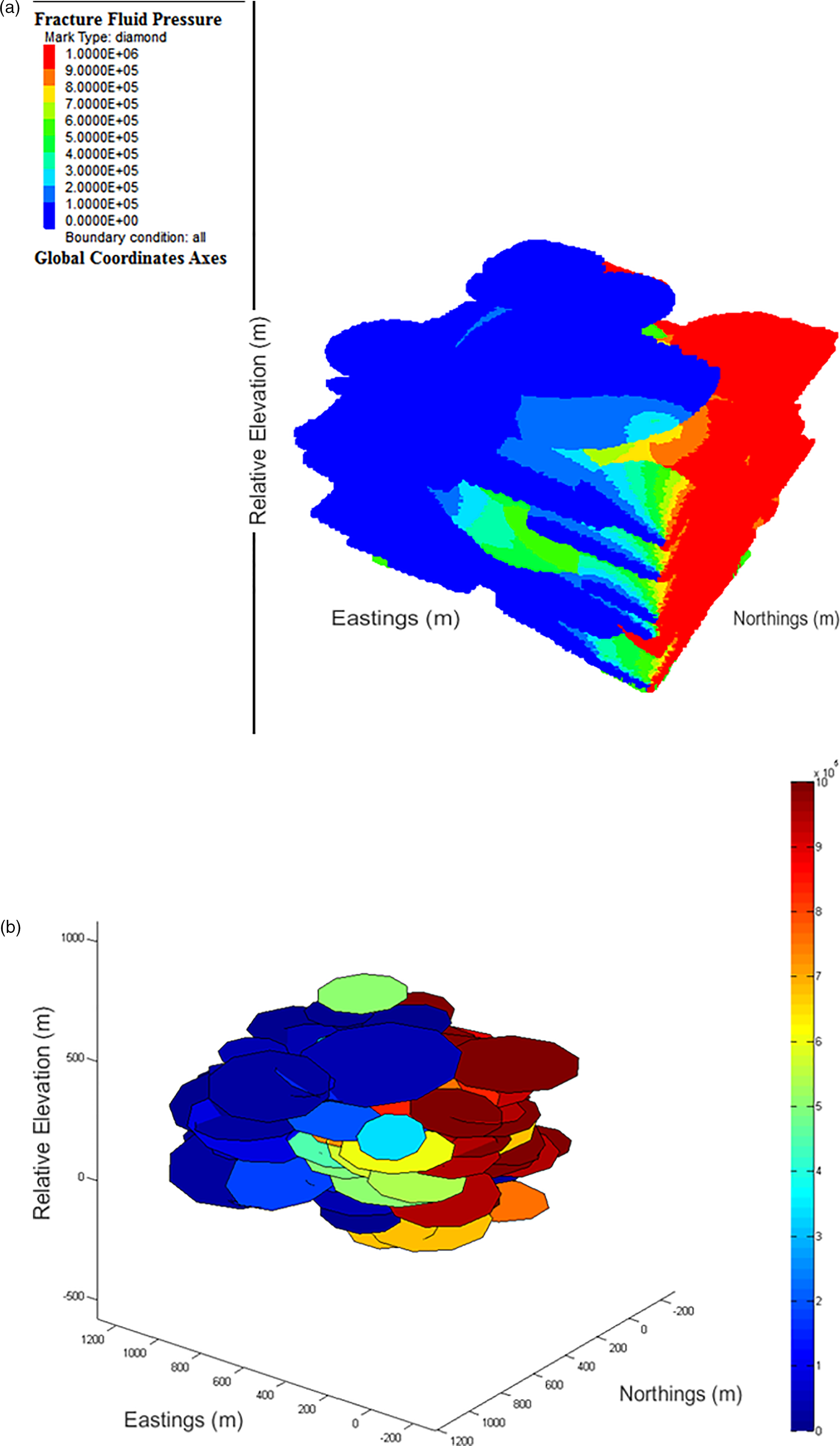
A comparison of visualisations from the numerical code a and Qsum b indicating that the fluid pressures show good agreement. Note that Qsum has coloured the isolated fractures at the top (green) and middle (light blue) differently to the numerical code as these fracture join two boundaries with incompatible boundary conditions

Example application – rapid characterisation of uncertainty in permeability as a function of uncertainty in fracture orientation

To demonstrate the value of the proposed method, the 3D fracture network geometry presented in Full 3D simulations section was analysed to determine the sensitivity of the uncertainty in flow predictions as a function of uncertainty in fracture orientation. For the analysis present in Full 3D simulations section, a low degree of uncertainty was assumed for the fracture orientations (namely a Fisher's constant of κ = 50, equating approximately to a normal distribution standard deviation of 11°). Estimation of orientation uncertainty associated with a set of discontinuities is particularly challenging when limited borehole data are available. Further, when one recognises that for any given fracture, the borehole samples a small section, which undoubtedly does not characterise the non-planarity of the fracture. For the case where fracture networks are inferred from other means, such as microseismic monitoring (Xu et al. 2012), this uncertainty increases.

To analyse this effect, scenarios corresponding to different κ values were simulated as summarised in Table 4. Other simulation parameters were unchanged as listed in Table 3. Boundary conditions consisted of a 1 MPa pressure gradient in the x-direction and impermeable boundaries in the y- and z-directions. Since no numerical modelling needed to be performed in this analysis, the number of realisations per scenario was increased to 100.

Table 4

Scenarios modelled to represent uncertainty in Fisher's constant and observed variance in Qsum metric

Fisher's κ constant	Qsum (mean ± SD) pseudo-units
1	0.317 ± 0.040
25	0.251 ± 0.046
100	0.174 ± 0.043
1000	0.114 ± 0.032

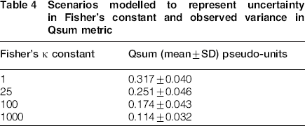
The results from Table 4 are shown in Fig. 14. The mean value of the Qsum flow metric decreases by a factor of three as the variance in the fracture orientations decreases (i.e. increasing κ parameter). This is because opportunities for fracture connectivity in this network of sub-horizontal fractures decrease as the orientation variance decreases and the fractures become more parallel. However, as shown in Fig. 14b, the coefficient of variance increases because although the absolute value of variance is not strongly dependent on κ, the mean value of the Qsum flow metric shows strong negative correlation. This demonstrates that the proposed method is computationally efficient and allows probabilistic sensitivity analyses that described above to be performed quickly.

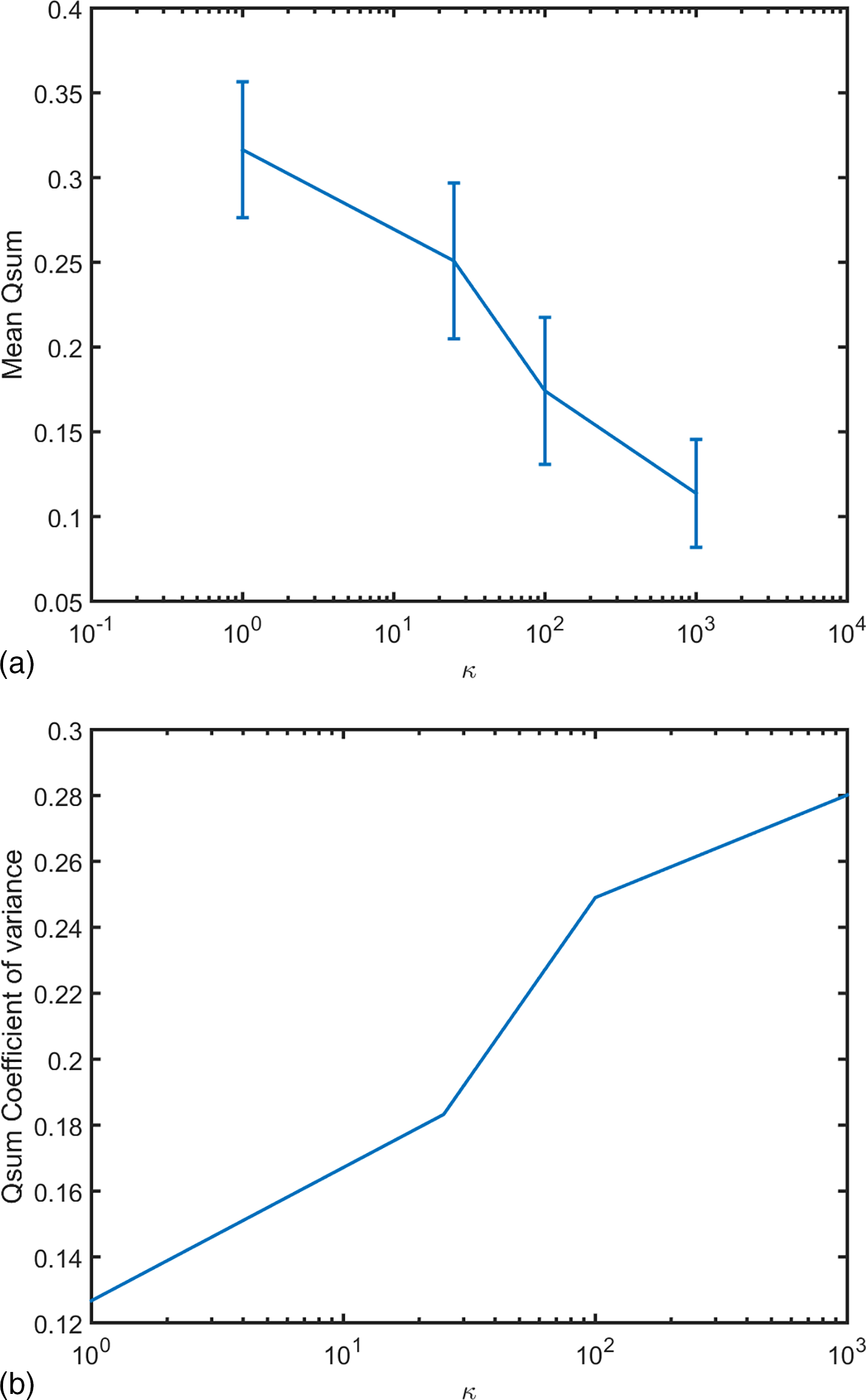
Evolution of uncertainty in the Qsum metric as a function of Fisher constant: a mean and standard deviation error bars for Qsum vs κ and b Qsum coefficient of variance as a function of κ

Application to slope stability analyses

The application of this method to slope stability analyses has also been investigated in a qualitative way.

Background

As previously highlighted, using DFNs rather than equivalent continuum methods involves a trade-off between the size and complexity of the simulated fracture networks and the computation time required for the analysis. There has been motivation to develop efficient techniques for performing first-pass geotechnical analyses before undertaking more complex numerical analyses. Polyhedral modellers have become more prevalent and provide a way to use these DFN for first pass analyses, such as key-block, limit-equilibrium stability analyses, estimations of block size distributions (BSDs) and rockfall hazard analysis (Lambert et al. 2012). They can also provide ‘seed’ geometries for more detailed modelling of stress and fracture evolution in the rock mass. The combination of probability or stochastic theory with polyhedral modelling has been shown to provide a powerful method for estimation of BSDs (e.g. Elmouttie and Poropat 2012) and (in combination with key-block theory) representation of the rock mass (e.g. Young and Hoerger 1989; Mauldon 1995). Sophisticated block tracing algorithms have been developed to accommodate these geometries using certain assumptions, such as assumed definition of polyhedral based on 2D traces (Song, Lee and Seto 2001), limitations to the maximum complexity of polyhedra (Menéndez-Díaz et al. 2009) and limitations of the shape of the simulation volume and the forced inclusion of at least some persistent fractures in the DFN (Lin, Fairhurst and Starfield 1987).

The block theory developed by Goodman and Shi (1985) has provided the framework for requirements for accurate detection and characterisation of generalised polyhedra. Several different approaches have been described for the estimation of in situ polyhedra and their properties, such as volume and shape, including the original and updated stereographic methods (Li, Xue, Xiao and Wang 1992), stereological (Maerz and Germain 1996), stereo-analytical (Zhang and Kulatilake 2003), grid-based trace analysis (Song et al. 2001) and block decomposition-based algorithms (Yu, Ohnishi, Xue and Chen 2009).

Development of a geometrical topology-based algorithm capable of handling generalised polyhedra without simplifications or approximations was shown in Lin et al. (1987) and Ikegawa and Hudson (1992). Further work to refine the algorithm to handle curved discontinuities, internally isolated voids, generalised boundary surfaces and to deal with robustness issues was described in Jing and Stephansson (1994), Jing (2000), Lu (2002), Elmouttie, Poropat and Krähenbühl (2010). The latter has been developed by the authors and treats all input polygons as potential polyhedral facets. It can accommodate arbitrary free surfaces (e.g. underground excavations, open pit excavations) and the existence of polygons (fractures) not responsible for formation of polyhedra can be treated as a measure of the internal polyhedron fracture frequency. Modern implementations of the algorithms are now capable of generating rock mass models involving hundreds of thousands of fractures, including non-planar structures, with the formation of equally vast numbers of polyhedra (rock blocks).

Potential metrics

Based on the authors’ experience in the aforementioned research, several metrics were assessed for suitability in selecting DFN realisations for slope stability analyses. They were polyhedral model BSD, BSD modified for internal fractures (BSD_i), and polyhedral model limit equilibrium analysis using progressive failure analysis (BSD^le). For metrics calculated using BSDs modified for both internal fractures and including the results of the limit equilibrium analysis, the notation is used.

The BSD metric was calculated using the volumes of the polyhedra generated from each DFN realisation. Polyhedra attached to the boundary surfaces of the model (base, back and sides) were excluded. The BSDⁱ metric was calculated by modifying the polyhedral volumes used in the BSD metric according to the number of internal (non-block forming) fractures within each block such that (7) where V′ is the modified volume, V the original polyhedral volume and n the number of internal fractures. For example, a block with a single internal fracture would now be represented as two blocks each with half the original volume.

The BSD^le metric was calculated by limiting the polyhedra used, to those assessed as kinematically unstable. This was assessed via a rigid block limit equilibrium stability analysis. No in situ stress field was modelled, although a progressive failure analysis was applied by assessing daylighting polyhedra for stability, removing unstable polyhedra and reassessing the polyhedra daylighting on the newly exposed surface.

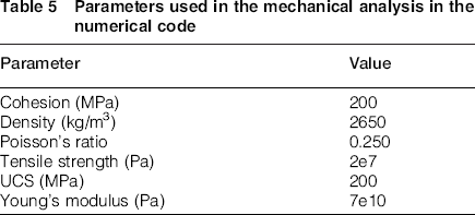
For the DFN generation and polyhedral modelling, the Siromodel software developed by CSIRO was used. The DFN were then imported into the lattice mechanics code ‘Slope Model’ for mechanical analysis. The parameters used were those associated with the default rock type available in Slope Model and are shown in Table 5. For the purposes of this analysis, the particular parameter values were not deemed to be of great importance.

Table 5

Parameters used in the mechanical analysis in the numerical code

Parameter	Value
Cohesion (MPa)	200
Density (kg/m³)	2650
Poisson's ratio	0.250
Tensile strength (Pa)	2e7
UCS (MPa)	200
Young's modulus (Pa)	7e10

A simple DFN geometry was used to validate the method of comparing the polyhedral analysis to the lattice mechanics simulations. A lattice resolution of 100 cm was used and a simulated time of 1 s (approximately 1 h compute time) was used. The geometry was based on a simple wedge failure and gradually modified to that of a complex wedge failure by reducing the persistence of one of the basal planes. This was performed to investigate the suitability of the method for use on rock masses experiencing composite failures.

Figure 15 shows an example of the visualisations of the polyhedral model (single wedge) and its lattice mechanics counterpart for a five-bench open pit excavation. As the persistence of one of the planes is reduced, the significance of the composite failure mechanism increases and the usefulness of the polyhedral representations decrease. Note that the version of Slope Model used for this work (2.9.9) did not permit the lowest bench of the model to be marked as mechanically free and so no failure is observed on this bench in the Slope Model simulations.

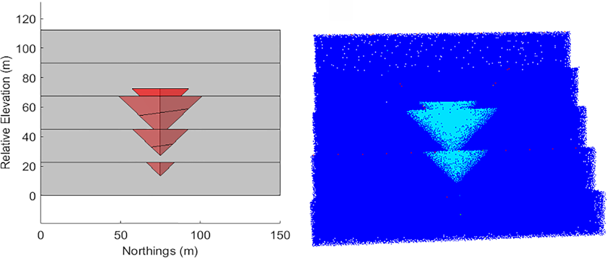
Single wedge discrete fracture network (DFN) realisation for a five-bench open pit excavation used in polyhedral (left) and lattice mechanics (right) analyses

Multiple bench analysis

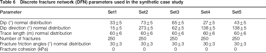
The method has been applied to the slope stability analysis of a synthetic case consisting of five benches of an open pit excavation. The DFN parameters have been chosen to promote a fragmented rock mass and the parameters are shown in Table 6. Trace length has been used to derive fracture radius for each set included in the DFN assuming circular fractures.

Table 6

Discrete fracture network (DFN) parameters used in the synthetic case study

Parameter	Set1	Set2	Set3	Set4	Set5
Dip (°) normal distribution	33 ± 5	73 ± 5	65 ± 5	27 ± 5	43 ± 5
Dip direction (°) normal distribution	15 ± 5	273 ± 5	62 ± 5	138 ± 5	138 ± 5
Trace length (m) normal distribution	60 ± 6	60 ± 6	60 ± 6	60 ± 6	60 ± 6
Number of fractures	250	250	250	250	250
Fracture friction angles (°) normal distribution	30 ± 3	30 ± 3	30 ± 3	30 ± 3	30 ± 3
Fracture cohesion (kPa)	0	0	0	0	0

A Monte Carlo simulation involving 100 DFN realisations was performed. Block size distributions were calculated corresponding to the aforementioned metrics and these are shown in Fig. 16a. There is significant variance in both the range and shape of the curves.

a BSD, b BSD_i, c BSD^le and d curves

From these BSDs, 90th percentile values from the individual curves where extracted to act as representatives for the metrics and these are shown in Fig. 17. The ordering of the simulations based on the different metrics show some similarity but there is sufficient variance to highlight the importance of choosing the correct metric for the particular analysis being undertaken.

a 90th percentile values from the individual BSD, b BSD_i, c BSD^le and d curves

Each of the four metrics identified a different pair of DFN realisations as constituting the lower and upper bounds of the BSDs. These ‘tail’ DFN realisations were imported into the lattice mechanics code for analysis. At the time of writing, there was no functionality within the lattice mechanics code to report on the volume of failed material predicted so a qualitative comparison was performed and good agreement is seen for the metric (ignoring the lower-most bench). These results are shown in Fig. 18. There are some discrepancies and these are partly because of the relatively coarse lattice resolution used in the lattice mechanics code.

Comparison of polyhedral and lattice mechanics results for a upper tail and b lower tail discrete fracture network (DFN) realisations selected using the metric. Note that lower most bench in Slope Model is constrained such that blocks will not fail

Application for rock strength characterisation

As previously discussed, the Hoek–Brown criteria are one of the most widely used empirical methods for scaling rock strength, by the GSI classification of the rock mass. A deliberately subjective approach was taken in the development of the GSI chart; however, several authors have attempted to quantify the calculation. Cai et al. (2004) propose that the average block volume formed by the intersection of joints within the rock mass at a representative volume or larger can be related to the Y axis of the GSI chart. For three approximately orthogonal persistent joint sets, he proposes the relationship between block volume, V_b, joint spacing, s_i, and the angle between joint sets, γ_i, as follows.

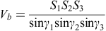
(8) An alternative quantification of the GSI chart is proposed by Hoek, Carter and Diederichs (2013) in which the values of the Y axis are a linear function of rock quality description [RQD (Deere, Hendron, Patton and Cording 1967)]. In this study, an investigation is made of the validity of these approaches and therefore of relevance is the mean and variance of block volumes and a representative linear measure of fracture frequency for estimation of a characteristic rock mass RQD.

The use of polyhedral block modelling (Elmouttie, Poropat and Hamman 2009) has shown that the average block volume calculation proposed by Cai et al. (2004) is valid with their assumption of joint persistence, i.e. fully or semi-persistent joints but significantly underestimates volumes for jointing with a more realistic assumption of joint size. In a paper in-press, we investigate the approach adopted by Hoek et al. (2013) and the use of the RQD. The authors conclude that a representative linear measure (fracture frequency correlated to RQD) can be derived via a reduction of the unbiased P32 (Dershowitz and Herda 1992) fracture intensity metric defined as the sum of joint areas normalised by the DFN volume. However, we observe that directly increasing joint persistence while keeping the P32 metric approximately constant (from a reduction in the total joint number) results in a near exponential reduction in rock mass strength. The authors conclude that the interconnection of the joint sets resulting from the increase in persistence is overwhelmingly the dominant factor in rock strength, not jointing intensity.

In this work, we take the study further and directly examine the influence on rock mass strength of the interconnection of jointing as measured by the Qsum metric. For a joint distribution, resulting in a backbone of interconnected fractures, we have demonstrated that the Qsum metric appears to correlate well with the fluid flux. For rock mass strength observations, we investigated the use of the metric to identify the percolation threshold and to examine the correlation between the Qsum metric and rock mass strength for fracture distributions above the percolation threshold. Use is made of SRM modelling to estimate the strength of samples composed of intact material and a DFN with typical joint properties. In this numerical rock analogue, the features identified as controlling rock mass strength are directly represented and the resultant rock mass strength and strength envelope are demonstrated to approximate well with empirical methods when the necessary conditions are satisfied.

The rock mass analogue consists of intact rock, a DFN and joint properties. To enforce isotropy in joint distribution 13 joint sets are defined at a local spatial orientation of 45°. Properties are presented in Tables 7 and 8. For the purposes of this comparative analysis, the mechanical properties used for joints were zero for cohesion and 0.5 for the coefficient of friction.

Table 7

Intact rock properties for sandstone sample

Lithology	Young's modulus (GPa)	UCS (MPa)	Tensile strength (MPa)
Sandstone	11.7	75.0	7.5

Table 8

Joint set orientations and lower hemisphere projection of the 13 joint sets (one being horizontal is not immediately obvious in the figure). Friction coefficient of 0.5 is applied to all joints

Joint set number	Dip direction (°)	Dip (°)	Joint diameter (m)	Lower hemisphere projection of joint sets
1	0	0	0.8
2	270	45	0.8
3	90	45	0.8
4	270	90	0.8
5	225	45	0.8
6	315	45	0.8
7	135	45	0.8
8	45	45	0.8
9	0	90	0.8
10	0	45	0.8
11	180	45	0.8
12	225	90	0.8
13	135	90	0.8

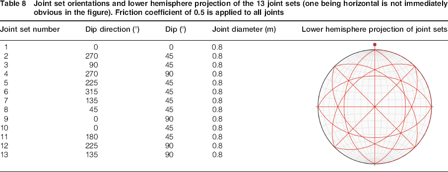
Eight realisations of the DFN are generated with the maximum number of joints per joint set varied between 50 and 300. By trial, these numbers were selected to span the onset of the development of the percolation backbone. Attributes of these DFNs including the Qsum metric and estimated strength (see below) are presented in Table 9.

Table 9

Joint density, Qsum and P32 metrics and estimated mass strength from synthetic rock mass (SRM) modelling

Joints/set	Total joints in 5 m cube	Qsum	P32	Estimated mass strength (MPa)
50	640	0.000	1.790	26.04
75	960	0.000	2.604	20.93
100	1273	0.000	3.545	15.51
125	1592	0.000	4.462	14.23
130	1653	0.198	4.618	13.78
150	1908	0.259	5.272	13.14
200	2556	0.503	6.977	10.54
300	3805	1.044	10.515	6.18

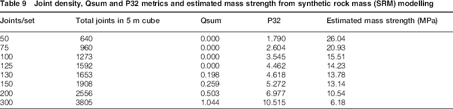
Each sample is subject to unconfined compression parallel with the Z axis and the peak strength recorded. A previous study had estimated that the representative rock mass size for a similar rock analogue was 3 m cubed and therefore for each DFN realisation two cubic samples with side lengths of 3 and 4 m centrally located within the 5-m cubic DFN domain was tested. Results are presented in Table 9, Figs. 19 and 20. In Fig. 19, a data point for each of the samples is shown. However, for clarity, in Fig. 20 (and later in Fig. 21), a single plot point is shown for each DFN realisation representing the mean value of the mass strength per pair of samples (error bars smaller than the size of the plot points).

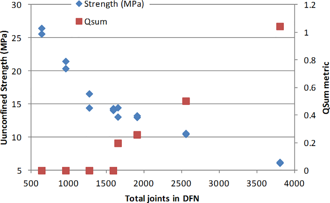
Mass strength and Qsum metric vs total joints in discrete fracture network (DFN) domain. Mass strength is calculated for centrally located cubic samples of 3 and 4 m side length for each DFN realisation

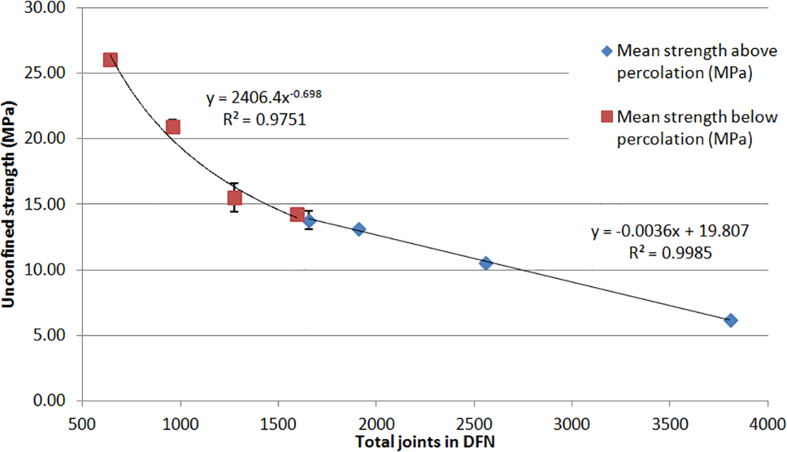
Mass strength (mean of two samples) vs total joint number with fitted trend lines above and below the percolation threshold

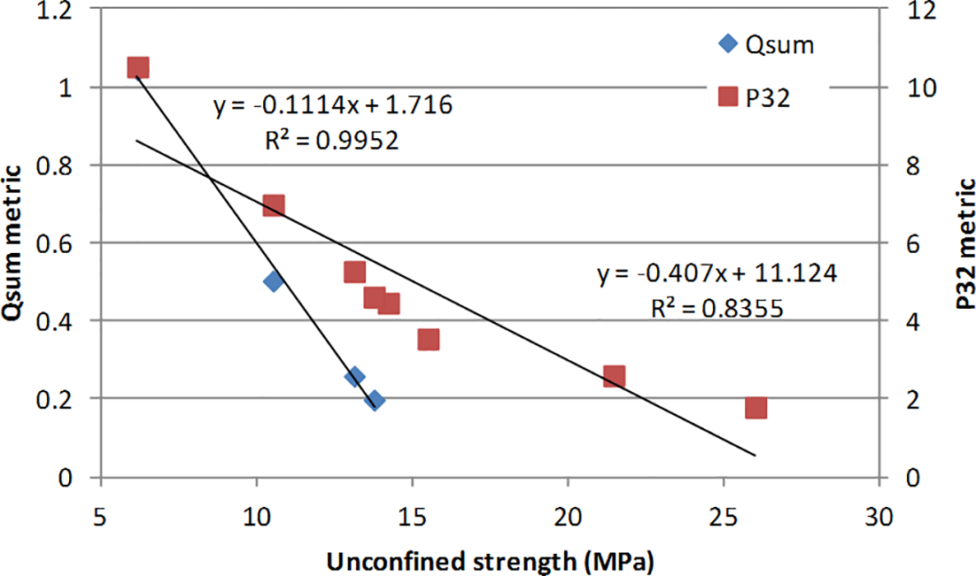
Relationship between Qsum and rock mass strength above the percolation threshold and P32 and rock mass strength over the studied range of jointing intensity

From the preliminary investigation on the use of these metrics for characterisation of rock mass strength, we draw the following observations. In terms of unconfined mass strength, we have observed a different response above and below the percolation threshold. Above the threshold the increase in jointing is apparently increasing the connected pathways. In an analogy with fluid flow, this is increasing the total flow between boundaries, as measured by the Qsum metric and also increasing the potential failure pathways as measured by the unconfined strength. A near linear relationship (R² ≈ 1.0) is observed between mass strength and Qsum (Fig. 21). Therefore, for the scenario where the fracture network realisations being assessed are above the percolation threshold in the direction of interest (in this case, vertically for comparison with UCS values), this metric can be a valuable guide for choosing DFN realisations for further analysis.

Below the percolation threshold, we observe the rock mass strength, increasing with an approximate power relationship with the reduction in joint density. While the Qsum metric is of no use below the percolation threshold, the ability to quickly identify this threshold for a specific DFN realisation is fundamental when discussing rock mass strength, joint density and joint intensity.

By comparison, the best measure of joint intensity, the unbiased P32 metric, is only of use above or below the percolation threshold with a bi-linear relationship with strength and inflection at this point (Fig. 21). By itself, the P32 metric cannot identify the percolation threshold.

Authors conclude that methods to quantify the GSI chart using simple statistical estimates of block volume or RQD have limitations as neither method addresses the true complexity of multiple interconnected joints sets of potentially variable persistence or satisfactorily addresses sampling biases. However, DFN modelling and simple metrics offer the potential of overcoming these limitations. Authors have demonstrated linear relationships between these metrics and rock mass strength as well as the influence of the percolation limit in delineating a different rock mass response to joint density.

Conclusions

The DFN method facilitates the analysis of rock mass heterogeneity when equivalent continuum representations are insufficient because of the problem of scale or fracture network properties. The method necessitates the use of multiple DFN realisations and computational load is often a limiting factor. In this paper, authors have demonstrated that the efficacy of using fast-to-compute, geometry-based metrics to select a small number of DFN realisations for the characterisation of uncertainty in hydrogeological, slope stability and geomechanical modelling. Additional work is required to further validate the approach for more complex fracture network geometries and for applicability to more complex physical processes, such as fracture propagation in hydraulic stimulation of reservoirs and rock mass failure for slope stability analysis.

Acknowledgements

This paper was originally presented at the first International Conference on Discrete Fracture Engineering (DFNE 2014) (19–22 October 2014, Vancouver, BC, Canada) and has subsequently been revised and extended before consideration by Mining Technology. The authors are grateful to Andy Wilkins for his valued technical advice and for Itasca for their technical support. Authors would also like to thank Manoj Khanal, Jane Hodgkinson and the anonymous reviewers for their help in improving the manuscript.

References

Cacas

M. C.

, Ledoux

, De Marsily

and Tillie

1990. Modelling fracture flow with a stochastic discrete fracture network: calibration and validation, Water Sources Research, 26, (3), 479–489.

Cai

, Kaiser

P. K.

, Uno

, Tasaka

and Minami

2004. Estimation of rock mass deformation modulus and strength of jointed hard rock masses using the GSI system, International Journal of Rock Mechanics and Mining Science, 41, 3–19.

Cundall

P. A.

2008. A new approach to the DEM, with applications to brittle, jointed rock, Aussois, ALERT School.

Deere

D. U.

, Hendron

A. J.

, Patton

F. D.

and Cording

E. J.

1967. Design of surface and near surface construction in rock. In:Failure and breakage of rock, proc. 8th U.S. symp. rock mech, (ed. Fairhurst

., New York, Soc. Min. Engrs, Am. Inst. Min. Metall. Petrolm Engrs, 237–302.

Dershowitz

W. S.

and Fidelibus

1999. Derivation of equivalent pipe network analogues for three-dimensional discrete fracture networks by the boundary element method, Water Resources Research, 35, (9), 2685–2691.

Dershowitz

W. S.

and Herda

H. H.

1992. Interpretation of fracture spacing and intensity. In:The 33rd U.S. Symposium on Rock Mechanics. 3-5 June, Santa Fe, New Mexico, 757–766.

Elmouttie

M. K.

and Poropat

G. V.

2012. A method to estimate in situ block size distribution, Rock Mechanics and Rock Engineering, 45, (3), 401–407.

Elmouttie

, Poropat

and Hamman

2009. Simulations on the sensitivity of rock structure models to field mapped parameters, in Slope Stability, Santiago Chile.

Elmouttie

, Poropat

and Krähenbühl

2010. Polyhedral modelling of rock mass structure, International Journal of Rock Mechanics and Mining Science, 47, (4), 544–552.

10.

Goodman

R. E.

and Shi

G.-H.

1985. Block theory and its application to rock engineering, New Jersey, Prentice Hall.

11.

Hoek

and Brown

E. T.

1980. Empirical strength criterion for rock masses, Journal of Geotechnical Engineering, 106, 1013–1040.

12.

Hoek

and Brown

E. T.

1997. Practical estimates of rock mass strength, International Journal of Rock Mechanics and Mining Science, 34, 1165–1186.

13.

Hoek

, Carter

T. G.

and Diederichs

M. S.

2013. Quantification of the geological strength index chart, in 47th US Rock Mechanics/Geomechanics Symp, 23–29, San Francisco, USA.

14.

Hoek

, Marinos

and Benissi

1998. Applicability of the geological strength index (GSI) classification for weak and sheared rock masses – the case of the Athens schist formation, Bulletin of Engineering Geology and the Environment, 57, (2), 151–160.

15.

Ikegawa

and Hudson

J. A.

1992. A novel automatic identification system for three-dimensional multi-block systems, Engineering Computations, 9, 169–179.

16.

Jing

2000. Block system construction for three-dimensional discrete element models of fractured rocks, International Journal of Rock Mechanics and Mining Science, 37, 645–659.

17.

Jing

2003. A review of techniques, advances and outstanding issues in numerical modelling for rock mechanics and rock engineering, International Journal of Rock Mechanics and Mining Science, 40, 283–353.

18.

Jing

and Stephansson

1994. Topological identification of block assemblages for jointed rock masses, International Journal for Numerical and Analytical Methods Geomechanics, 31, 163–172.

19.

Lambert

, Thoeni

, Giacomini

, Casagrande

and Sloan

S. W.

2012. Rockfall hazard analysis from discrete fracture network modelling with finite persistence discontinuities, Rock Mechanics and Rock Engineering, 45, (5), 871–884.

20.

, Xue

, Xiao

and Wang

1992. Block theory on the complex combinations of free planes, Computers and Geotechnics., 40, 127–134.

21.

Lin

, Fairhurst

and Starfield

A. M.

1987. Geometrical identification of three dimensional rock block systems using topological techniques, International Journal of Rock Mechanics and Mining Science, 24, (6), 331–338.

22.

Long

, Gilmour

and Witherspoon

P. A.

1985. A model for steady fluid flow in random three-dimensional networks of disc-shaped fractures, Water Resources Research, 21, (8), 1105–1115.

23.

2002. Systematic identification of polyhedral rock blocks with arbitrary joints and faults, Computer and Geotechnics, 29, 49–72.

24.

Maerz

N. H.

and Germain

1996. Block size determination around underground openings using simulations. In:FRAGBLAST 5 Workshop on Measurement of Blast Fragmentation, Montreal, Quebec, Canada, 23 – 24 Aug, 215–223, Balkema, Rotterdam.

25.

Marinos

and Hoek

2000. GSI: a geologically friendly tool for rock mass strength estimation. In:Proceedings of the GeoEng2000 at the International Conference on Geotechnical and Geological Engineering, Melbourne, Technomic publishers, Lancaster, 1422–1446.

26.

Mas Ivars

, Deisman

, Pierce

and Fairhurst

2007. The synthetic rock mass approach – a step forward in the characterization of jointed rock masses. In:Proceedings of the 11th congress on International Society of Rock Mechanics, (eds. Ribeiro e Sousa

and Grossmann

., London, Taylor & Francis, Vol. 1, 485–490.

27.

Mas Ivars

, Pierce

M. E.

, Darcel

, Reyes-Montes

, Potyondy

D. O.

, Young

R. P.

and Cundall

P. A.

2011. The synthetic rock mass approach for jointed rock mass modelling, International Journal of Rock Mechanics and Mining Science, 48, 219–244.

28.

Mauldon

1995. Keyblock probabilities and size distributions: a first model for impersistent 2-D fractures, International Journal of Rock Mechanics and Mining Science, 32, 575–583.

29.

Menéndez-Díaz

, González-Palacio

, Álvarez-Vigil

A. E.

, González-Nicieza

and Ramírez-Oyanguren

2009. Analysis of tetrahedral and pentahedral key blocks in underground excavations, Computers and Geotechnics, 36, 1009–1023.

30.

Odling

N. E.

, Gillespie

, Bourgine

, Castaing

, Chiles

J.-P.

, Christensen

N. P.

, Fillion

, Genter

, Olsen

, Thrane

, Trice

, Aarseth

, Walsh

J. J.

and Watterson

1999. Variations in fracture system geometry and theoretical implications for fluid flow in fractured hydrocarbon reservoirs, Petroleum Geoscience., 5, 373–384.

31.

Pettit

, Pierce

, Damjanac

, Hazzard

, Lorig

, Fairhurst

, Gil

, Sanchez

, Nagel

, Reyes-Montes

and Young

R. P.

2011. Fracture network engineering for hydraulic fracturing, The Leading Edge, 2011, 844–852.

32.

Pierce

, Cundall

, Potyondy

and Mas Ivars

2007. A synthetic rock mass model for jointed rock. Rock Mechanics: Meeting Society's Challenges and Demands, 1st Canada-U.S. Rock Mechanics Symposium, (eds. Eberhardt

, ). Vancouver, May 2007, Vol. 1, Fundamentals, New Technologies & New Ideas, Taylor & Francis Group, London, 341–349.

33.

Read

and Stacey

2009. Guidelines for open pit slope design, Clayton, CSIRO Publishing, 512 p.

34.

Slope Model User's manual, Itasca Consulting Group 0000.

35.

Song

J.-J.

, Lee

C.-I.

and Seto

2001. Stability analysis of rock blocks around a tunnel using a statistical joint modelling technique, Tunnelling and Underground Space Technology., 16, 341–351.

36.

, Dowd

and Mohais

2012. Connectivity analysis of the Habanero enhanced geothermal system. In:Proceedings 37th Workshop on Geothermal reservoir Engineering, Stanford University, Stanford California, Jan 30 – Feb 1, 2012, SGP-TR-194.

37.

Young

D. S.

and Hoerger

S. F.

1989. Probabilistic and deterministic key block analyses. In:Proceedings of the 30th U.S. Symposium on Rock Mechanics, (ed. Khair

A. W.

., Morgantown, 227–235, Balkema, Rotterdam.

38.

, Ohnishi

, Xue

and Chen

2009. A generalized procedure to identify three-dimensional rock blocks around complex excavations, International Journal for Numerical and Analytical Methods Geomechanics, 33, 355–375.

39.

Zhang

and Kulatilake

P. H. S. W.

2003. A new stereo-analytical method for determination of removal blocks in discontinuous rock masses, International Journal for Numerical and Analytical Methods Geomechanics, 27, 791–811.