Application of discrete fracture networks in mining and civil geomechanics

Abstract

Discrete Fracture Networks (DFNs) appear to be used differently in mining and civil applications. In mining, DFNs are used primarily within the context of Synthetic Rock Mass (SRM) models to estimate rock mass strength and deformation characteristics for use in mine-scale analysis of mass mining, i.e., cave mines and large open pits. Discrete Fracture Networks are also used in mining to estimate fragmentation distributions, kinematic block stability and groundwater flow into mines. Applications of DFNs in traditional civil engineering are perhaps less common than those in mining. However, more DFN-related research has been performed in support of nuclear waste repositories than for mining. This is because hydraulic properties of fractured rock and the associated flow prediction are of crucial importance for nuclear waste repositories. This paper attempts to highlight some of the developments of DFN applications in both mining and civil engineering. No attempt is made to delve into the details of DFN generation (e.g., scaling laws), but attention is given to some challenges faced in mining and civil geomechanics when trying to use DFNs.

Keywords

Synthetic rock mass (SRM)Discrete element method (DEM)Particle flow code (PFC)

Introduction

Failure and deformation process of rock masses surrounding underground and surface excavations has been a problem for centuries, but only recently have practical methods for analysing these problems gradually developed. Major increases in mineral production and civil engineering infrastructure development have resulted from demands of larger, more sophisticated and wealthier populations around the world. Larger and deeper excavations are required to meet these demands, and in mining, the concept of the mass mining started to be accepted as the most efficient and economical way in which to produce minerals, particularly from disseminated low-grade deposits. Very large open pit and underground caving operations have been planned and are being developed around the world. However, the design methods that were used from the 1940s to the 1990s are no longer acceptable. For example, empirical caving design methods that have long served the industry well for smaller mines were not adequate for the complex rock failure and deformation process in very large deep mines. This led to the introduction of Synthetic Rock Mass (SRM) models and methodologies aimed at a more robust understanding of the rock mechanics involved.

The backbone of SRMs is the discrete Fracture Network (DFN). Consequently the role of DFNs in civil and mining geomechanics has increased markedly in recent years. Before 2010, there was almost no mention of DFNs in papers of major conferences dealing with mass mining or open pits. In the last 3 years, these conferences have averaged six papers per conference. Most of the papers deal with the use of DFNs in SRM models. DFN applications in civil engineering have been focused for some time in fracture flow simulations in nuclear waste isolation studies. Although DFNs are important in flow studies, they are also important in excavation stability analyses. This paper attempts to highlight some of the developments of DFN applications in both mining and civil geomechanics. No attempt is made to delve into the details of DFN generation, but attention is given to some challenges faced in mining and civil geomechanics when trying to use DFNs.

Mining geomechanics applications

Discrete Fracture Networks have been used in mining geomechanics primarily in the following areas:

Synthetic Rock Mass models to estimate rock mass strength, fragmentation and microseismicity in caving mines, and to estimate anisotropic rock mass deformability and strength in open-pit mines.

Kinematic analysis of block stability in underground and open-pit excavations.

Determination of Equivalent Porous Media for flow estimates and pore pressure distributions in open-pit mines.

Direct evaluation of large-scale slope stability.

Each of these areas is discussed separately below.

SRM models

The ability of the SRM model to construct an ‘equivalent material’ that honours the strength of the intact rock and joint fabric within the rock bridges that may occur along a candidate failure surface in a closely jointed rock mass is a significant development. In particular, it provides a means of establishing a constitutive material model (strength envelope) that does not rely on either Mohr–Coulomb or Hoek–Brown criteria. This is particularly important in the case of anisotropic rock masses as discussed later in this section.

Historically, the Mohr–Coulomb measures of friction and cohesion have been used to represent the strength of a rock mass. This practice was based on soil mechanics experience and methodology, and assumed that the size of the rock particles in highly, closely jointed rock masses were equivalent to a mass of soil particles. This assumption enabled rock-slope design practitioners to adopt the Mohr–Coulomb measures of friction (Ø) and cohesion (c), and led to their embedment in the limit equilibrium stability analysis procedures that were introduced in the 1970s and 1980s. Determination of rock mass strength has been the holy grail of mining geomechanics ever since. At present, most practitioners determine the rock mass strength using the Hoek–Brown failure criterion. But this is gradually changing with the introduction of SRM methodologies.

The term ‘SRM’ was originated by the Mass Mining Technology (MMT) project to describe something very specific: In the context of the original definition, the intact rock is represented in three dimensions by the Discrete Element Method (DEM). SRM models attempt to reproduce the combined effects of intact fracture and discontinuity movement. Main inputs are intact rock properties, joint properties and a DFN.

Synthetic rock mass-like models are not new. For example, Carvalho, Kennard and Lorig (2002) used two-dimensional UDEC (Itasca Consulting Group, Inc 2004) models of diorite to estimate rock mass strengths for slope stability studies (see Figs. 1 and 2). Worthy of note is the observation that the failure mechanism in the triaxial samples was mainly a consequence of tensile failure of the intact rock bridges in the rock mass.

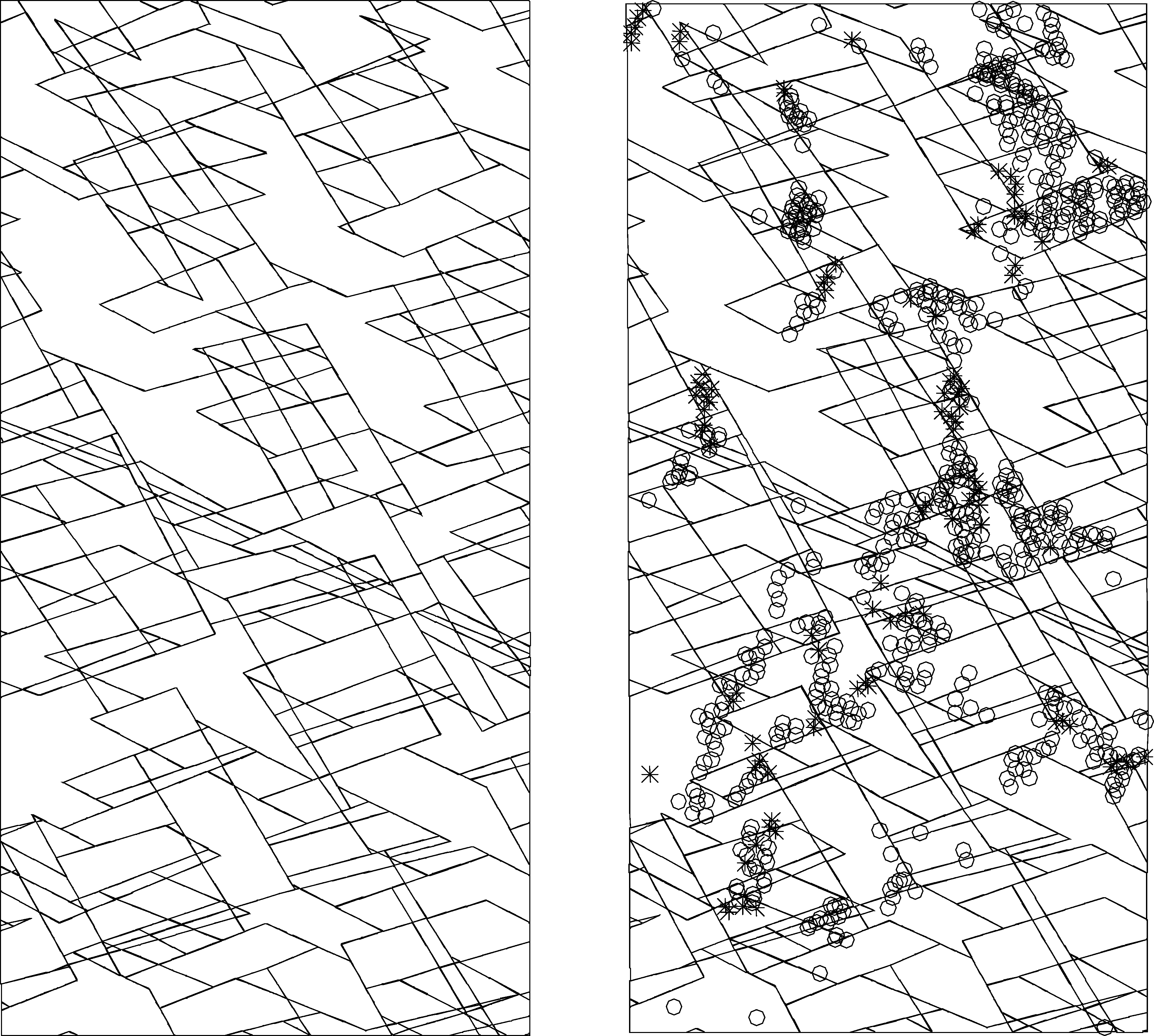
Rock mass sample: before (left) and after (right) numerical triaxial test (circles indicate tensile failure locations)

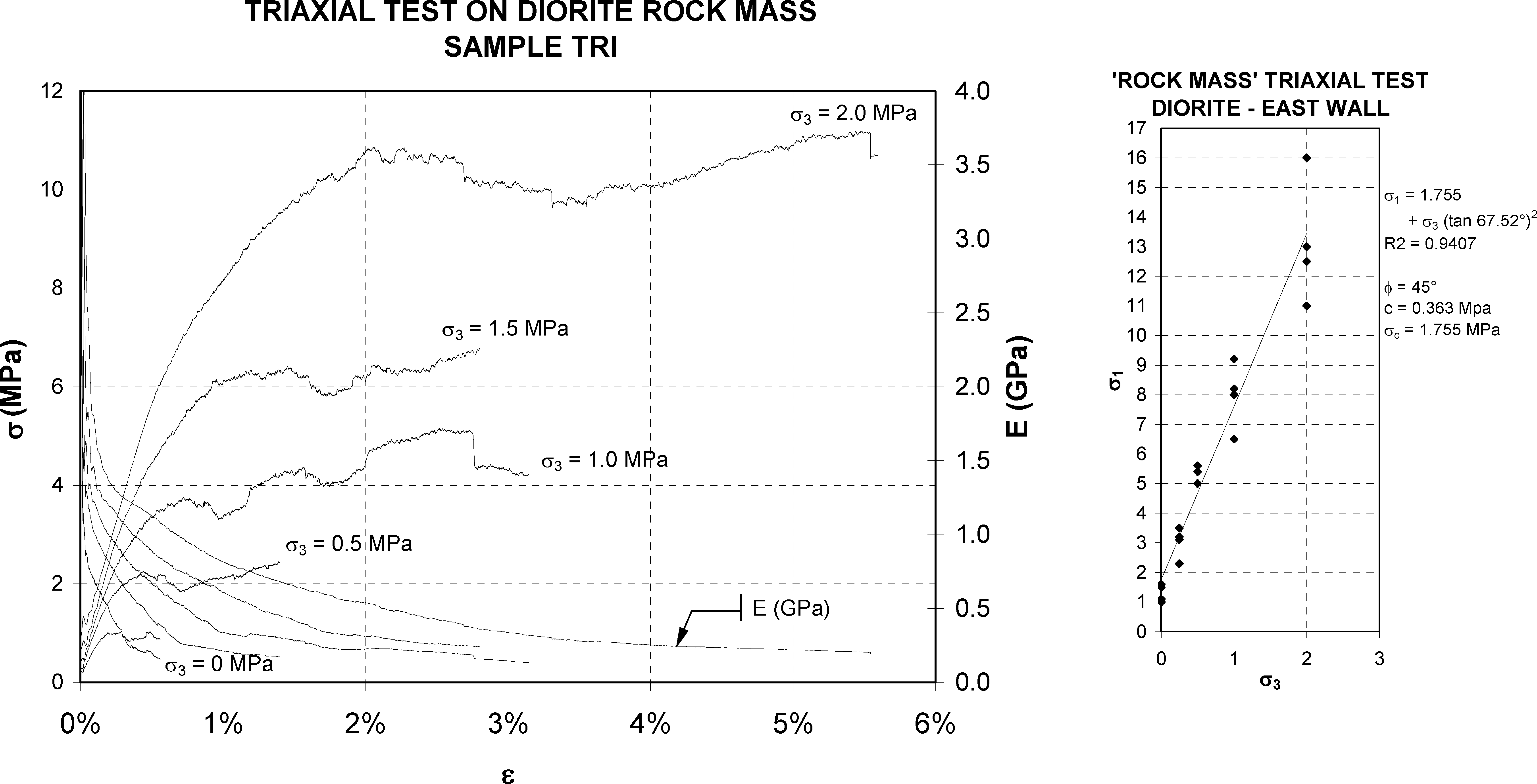
Rock mass sample: stress–strain curves (left) and Mohr–Coulomb envelope (right)

Clark (2006) used FLAC (Itasca Consulting Group, Inc 2011) with ubiquitous joints to construct an SRM-like model. The orientation of the ubiquitous joints was sampled from the actual distribution of joint orientations. The model exhibited anisotropy, scale effects and reasonably reproduced empirical strengths, as shown in Fig. 3.

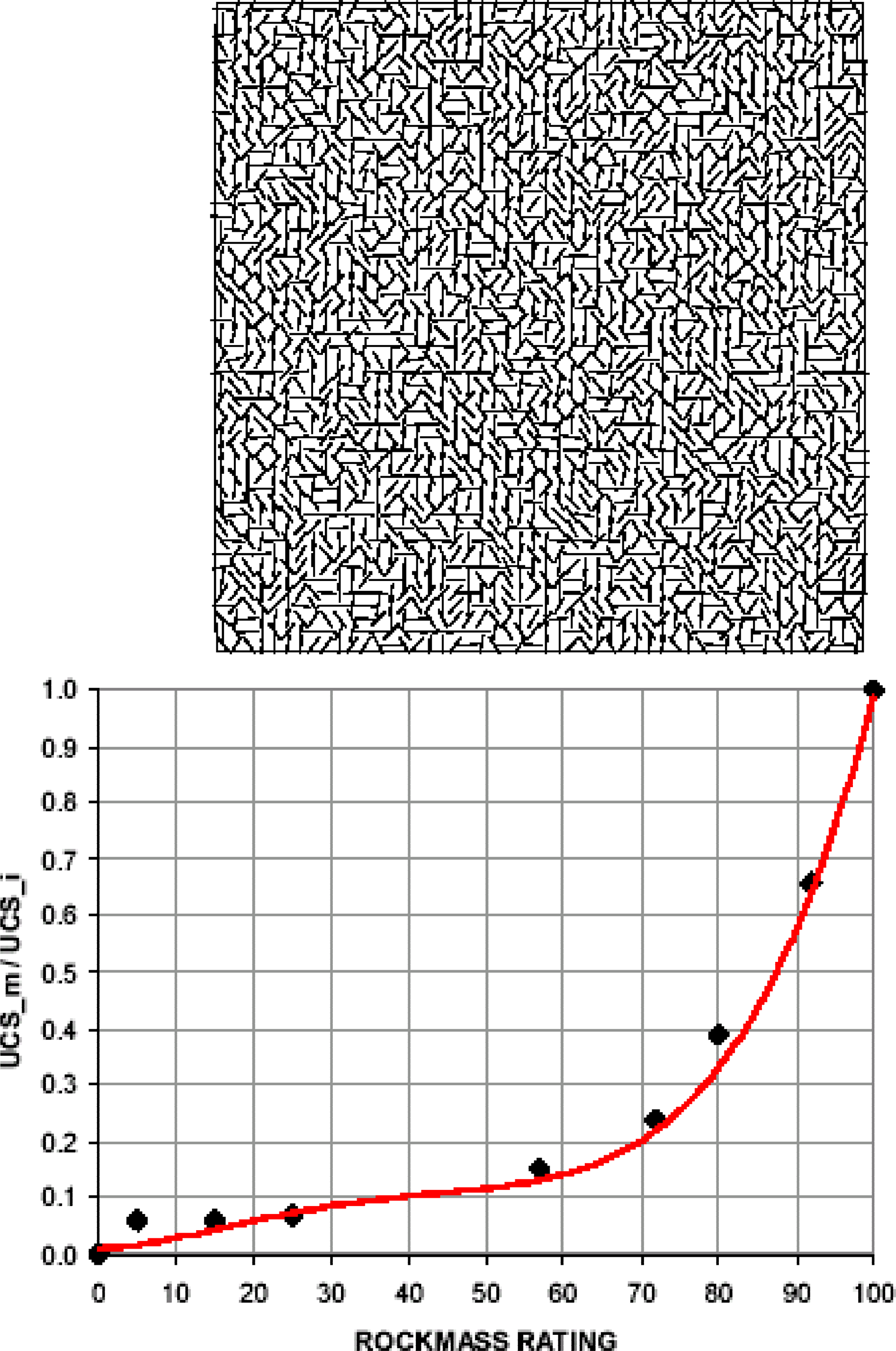
FLAC synthetic rock mass (SRM)-like model with four ubiquitous joint sets (top) and the SRM properties (shown as solid markers) compared against the empirical estimate of Barton (2000) as cited in Hoek (2004), shown as a solid line (bottom)

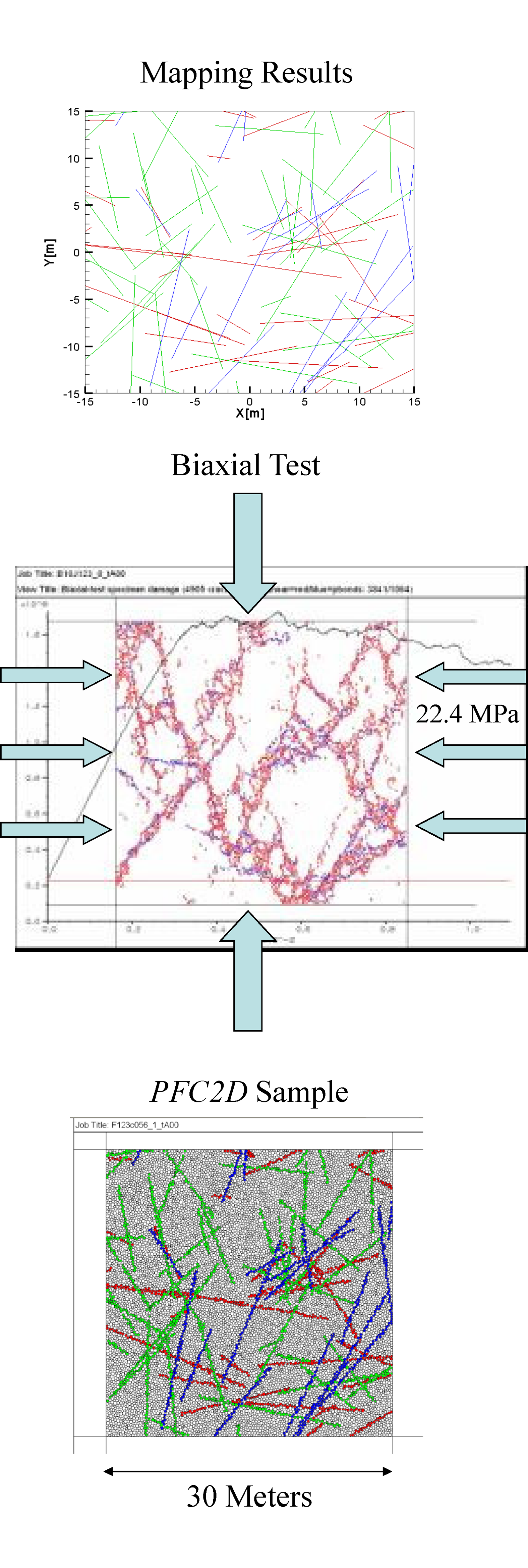
Park, Martin and Christiansson (2004) constructed SRM-like models with the Particle Flow Code (PFC2D) (Itasca Consulting Group, Inc 2014), as shown in Fig. 4. One limitation of this approach is that the joints were ‘bumpy’, with irregularities of the scale of the individual PFC particles. However, all of these early SRM-like models were constructed in 2D. It can be demonstrated that rock mass strength and fragmentation are likely to be severely underestimated in 2D SRM models. There are three main reasons for this:

Models incorporating 2D joint traces assume that fractures strike perpendicular to the plane of analysis (when in fact they may be subparallel).

The strike length of joints is represented as infinite in the out-of-plane direction.

Two-dimensional synthetic rock mass (SRM)-like model with PFC2D with ‘bumpy’ joints (Park et al. 2004)

Wing cracks can grow more freely from a two-dimensional crack than a three-dimensional crack. Damjanac, Gil, Pierce and Sanchez (2010) demonstrated that it is necessary to remove most of the joints from a 2D SRM model in order to obtain a rock mass strength that is consistent with a 3D SRM model. If this can be done, 2D SRM models can still provide good insight into potential failure modes.

Advances in PFC modelling of SRM models include:

extension of the modelling to three dimensions;

introduction of a ‘smooth joint’ contact model developed to overcome the ‘bumpy joint’ problem;

introduction of a ‘flat joint’ failure models that allow proper representation of both intact rock compressive and tensile strength; and

a more rapid testing methodology.

Although it would be ideal to construct and run full 3D caving simulations using explicit representations of the DFN, it is not computationally feasible. The most common approach is to test a 3D SRM sample (containing the field-derived DFN) and subject it to strain paths determined from a continuum (with faults) simulation. The resulting mechanical behaviour (notably brittleness, which depends on rock-bridge fracture) is then imported into the continuum model as a constitutive relation. The process is depicted graphically in Fig. 5.

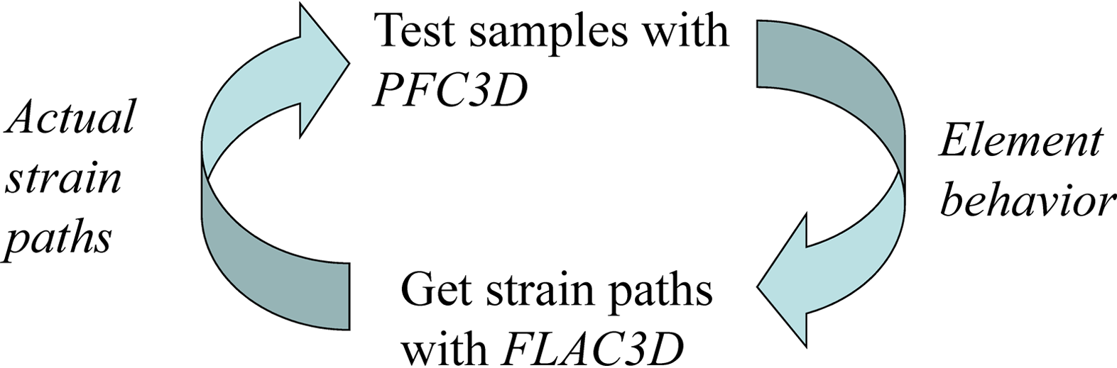
Synthetic rock mass (SRM) methodology in 3D

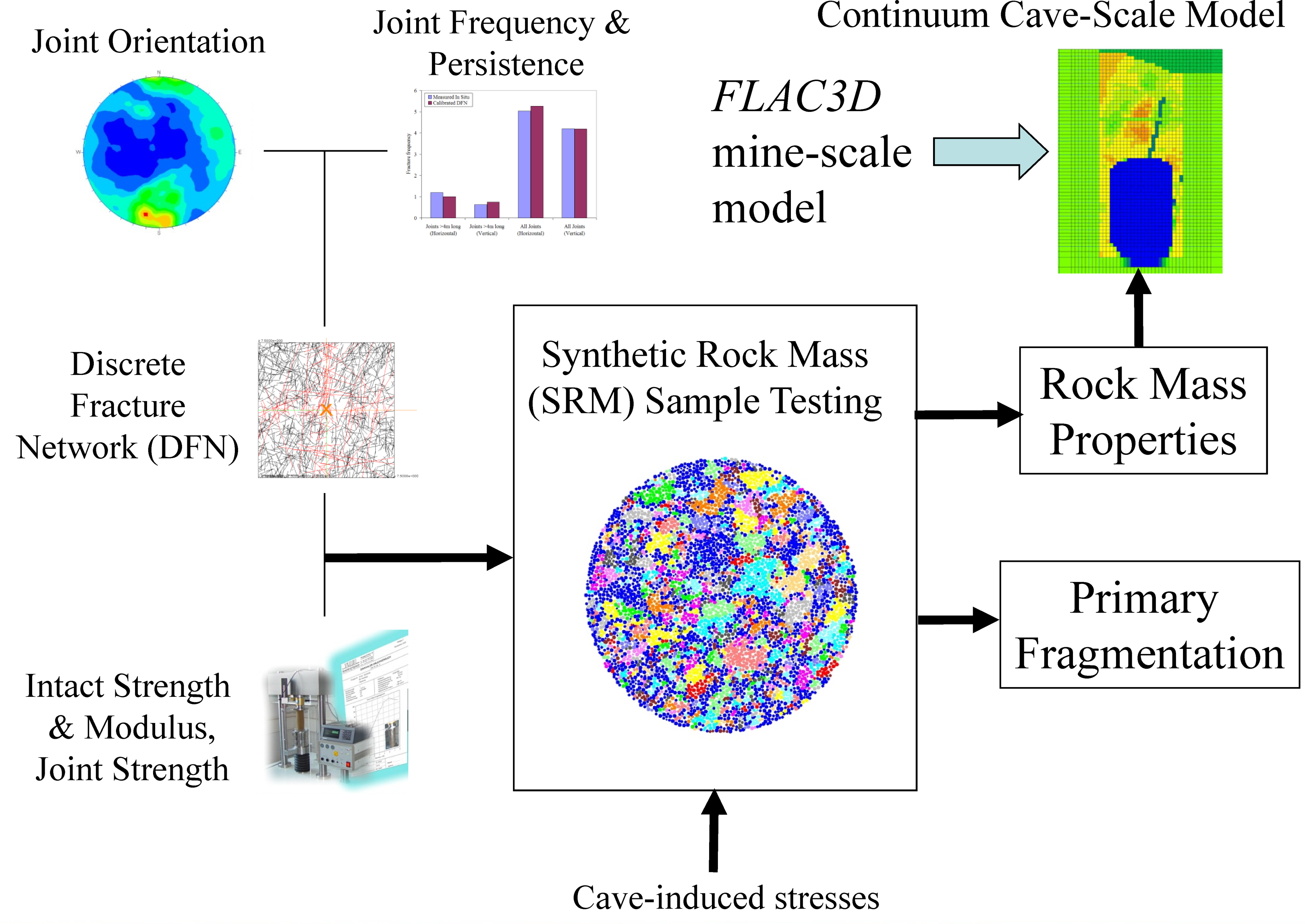
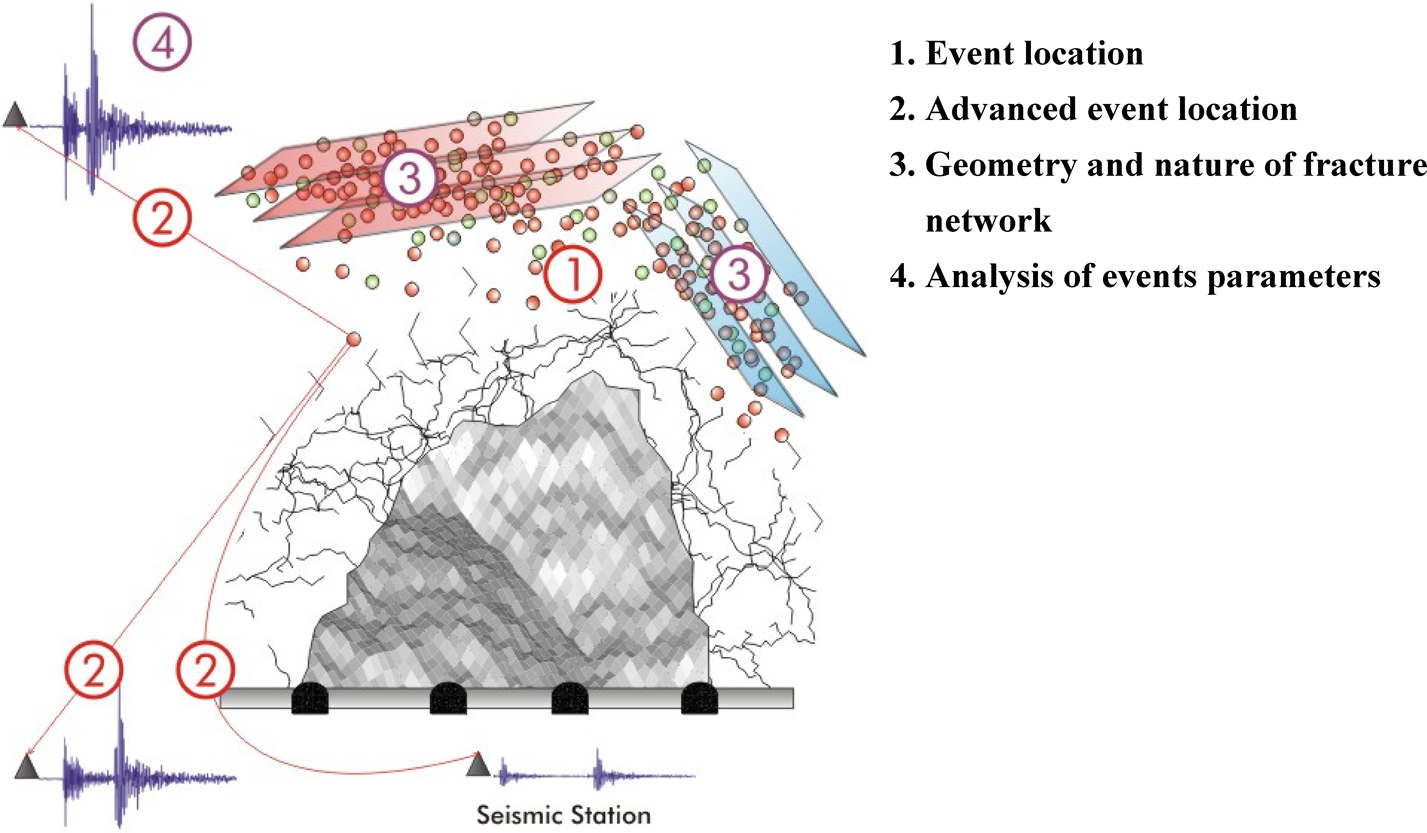
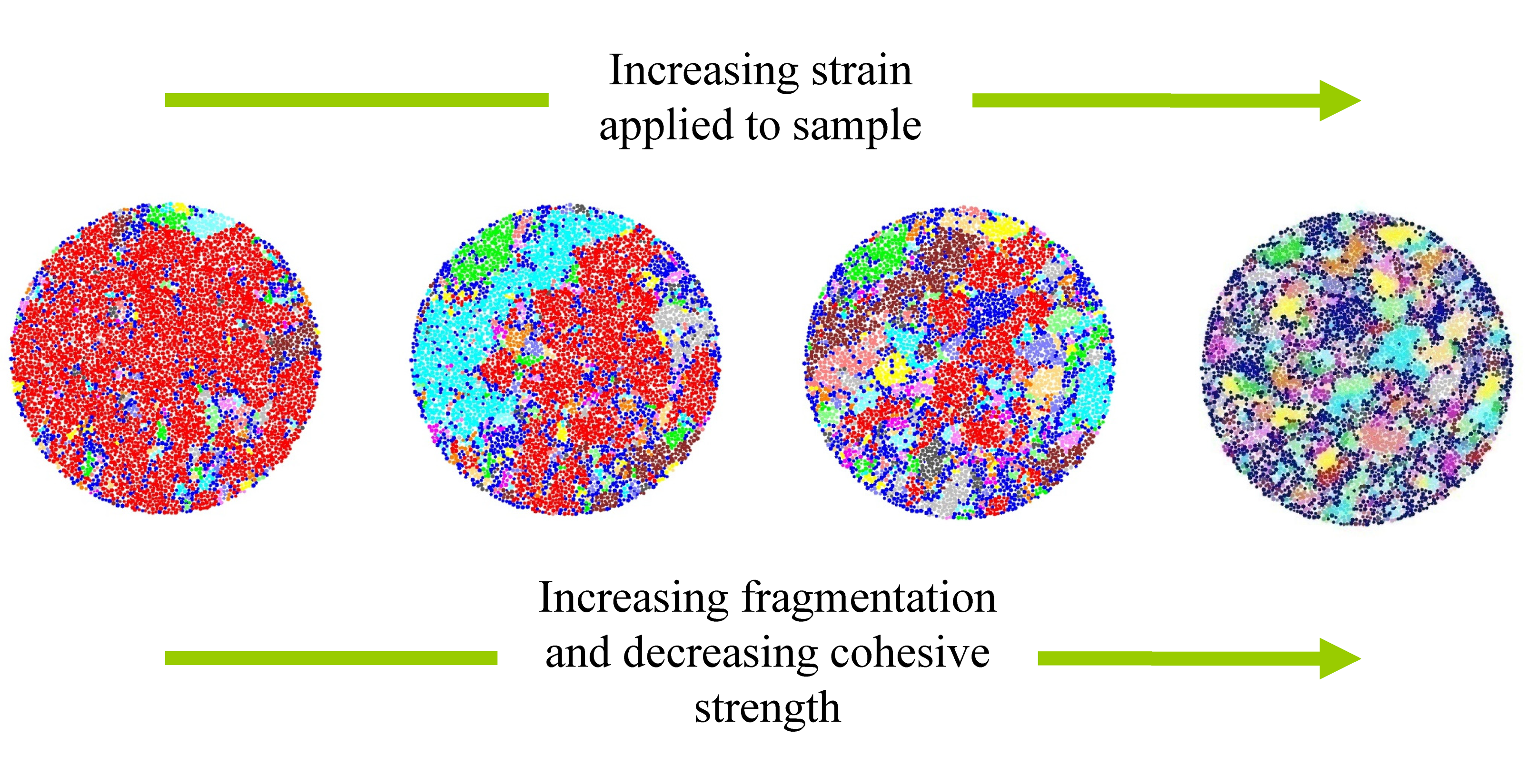
The rock response around a large block cave has been evaluated using this methodology, as shown in Fig. 6. The example comes from Lift 2 of Northparkes E26 mine. Validation of the methodology comes from the following three areas. 1.

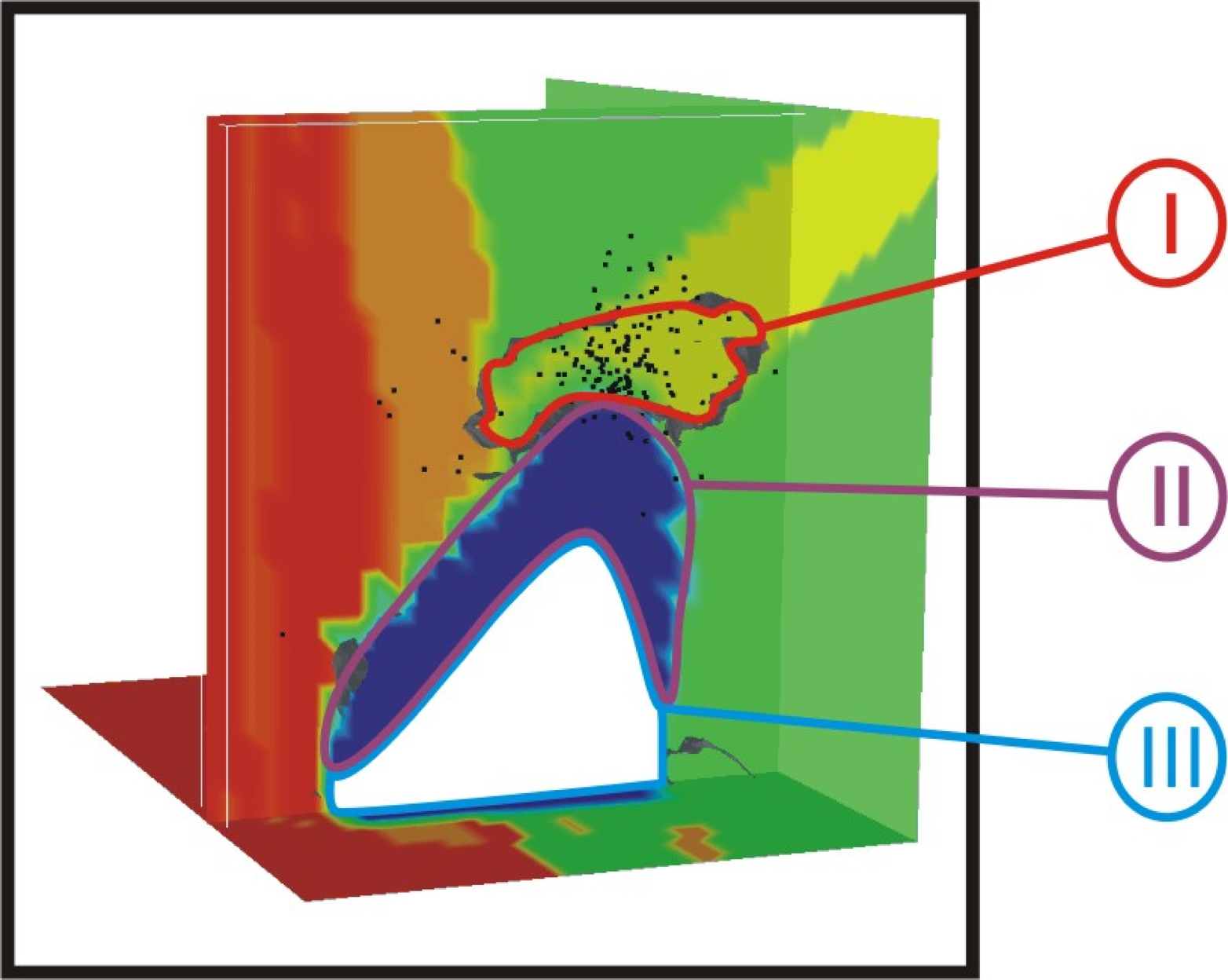
Induced Fractures – Compare fracture orientations from SRM tests with what may be inferred from microseismicity as shown in Fig. 7.

Fragmentation – Compare SRM test predictions with drawpoint observations as shown in Fig. 8.

Shape and Advance Rate of Cave – Compare cave-scale model predictions with in situ observations of seismogenic zone and yield zone as shown in Fig. 9.

Use of three-dimensional synthetic rock mass (SRM) in evaluating the rock response around a large block cave

Microseismic data for model validation [through studies by Reyes-Montes, Pettitt and Young (2007)] (1) event location (2) advanced event location (3) geometry and nature of fracture network (4) analysis of events parameters

Example of fragmentation (Mas Ivars et al. 2011) obtained by applying strain path to synthetic rock mass (SRM) sample. Solid shades denote contiguous blocks of bonded material (i.e., isolated intact rock blocks)

FLAC3D (Itasca Consulting Group, Inc 2012) model of cave showing seismogenic zone (I), yielded zone (II) and cave (III)

Besides the SRM methodologies, several studies were carried out to define relations between the DFN geometrical properties and the mechanical behaviour of fractured rocks. It was addressed through both theoretical and numerical approaches.

Based on the seminal papers of Kachanov (1987), Kachanov and Laures (1989), Le Goc et al. (2014) developed a dislocation-based numerical method to derive mathematical relations for the rock modulus based on the DFN alone. Initiated for the MMT project and continued thereafter, this approach showed that the effective modulus (ratio of rock mass to intact modulus) is directly related to the DFN geometry (as quantified by the percolation parameter, p) under tensile conditions (Fig. 10). In the work shown here, p, the DFN percolation parameter (Bour and Davy 1998), first describes the DFN connectivity level. It is related to the cube of the joint radii per unit volume of rock mass. p is potentially more sensitive to the presence of large persistent joints, which demonstrated to have the most significant impact on rock mass modulus and strength. The correspondence between p and the estimated rock mass modulus is remarkable and suggests that, when coupled with measures of joint quality/condition, p may represent the key link between the nature of jointing in a rock mass and rock mass modulus, strength and caveability. p is related to the DFN connectivity (Bour and Davy 1998) and in some sense it might be a measure of the ‘degree of interlock’ that is believed to be responsible for rock mass strength. Work is continuing to see if the relation can be extended to rock mass strength and compressive conditions.

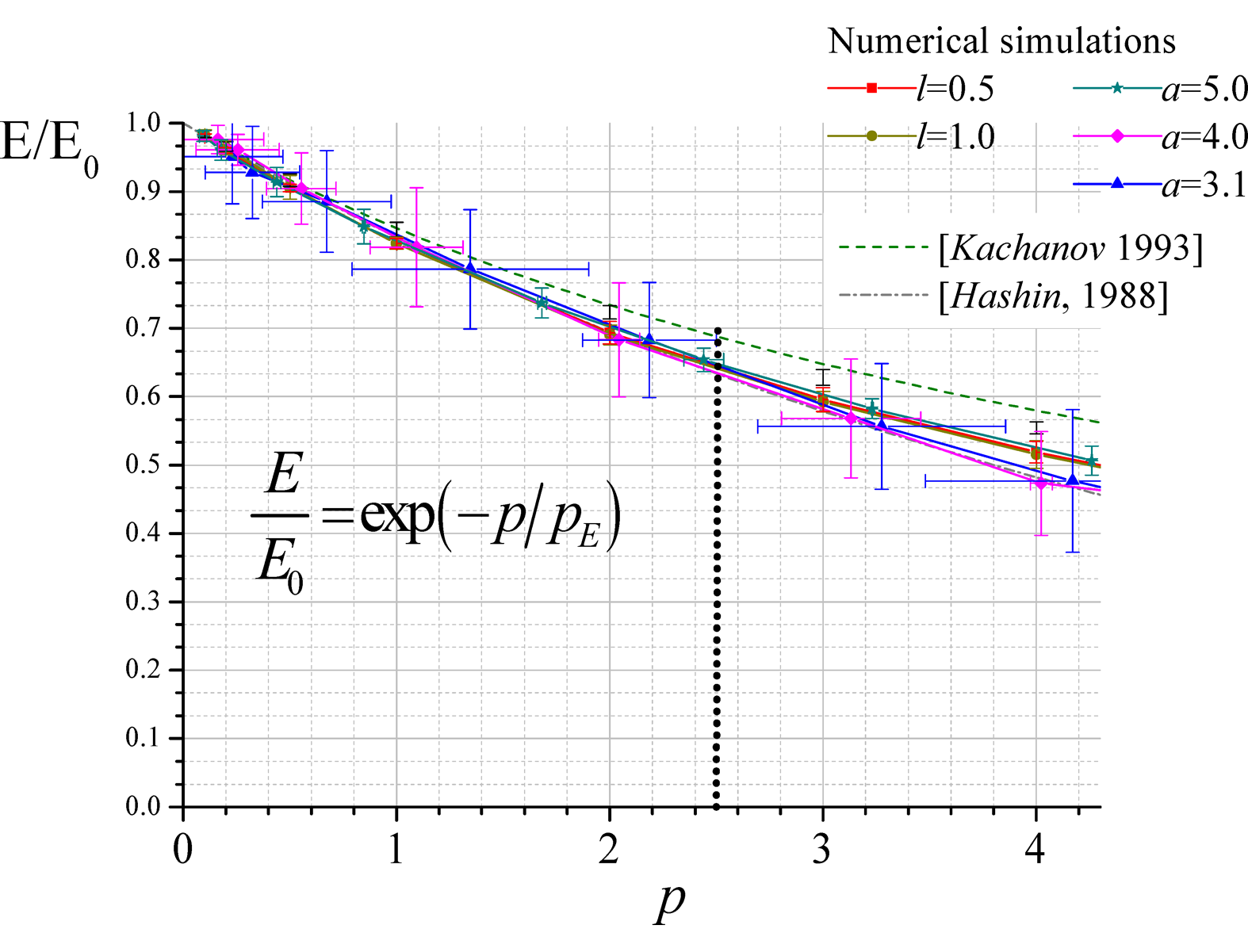
Relation between the effective Young's Modulus (rock mass modulus divided by intact rock modulus) and p (discrete fracture network (DFN) geometric property of fracture size to power 3) for a rock mass under tensile conditions. The relation is valid for a wide range of underlying size distributions (constant size l, power law of exponent a) and DFN model types [random disc, UFM (Davy et al. 2010)] and has been validated through complete simulations with 3DEC and PFC3D. From (Darcel, Davy and Le Goc 2013a, 2013b)

Nearly all rock masses are anisotropic to one degree or another. The strength and deformation behaviour of a rock mass is governed strongly by (a) the ‘intact’ strength of rock and (b) the presence of discontinuities such as joints, bedding planes, foliation, etc. Anisotropic rock mass strength and deformation behaviour result when a significant portion of the discontinuities is aligned in a preferred direction, such as the shale and banded iron formation rock masses shown in Fig. 11.

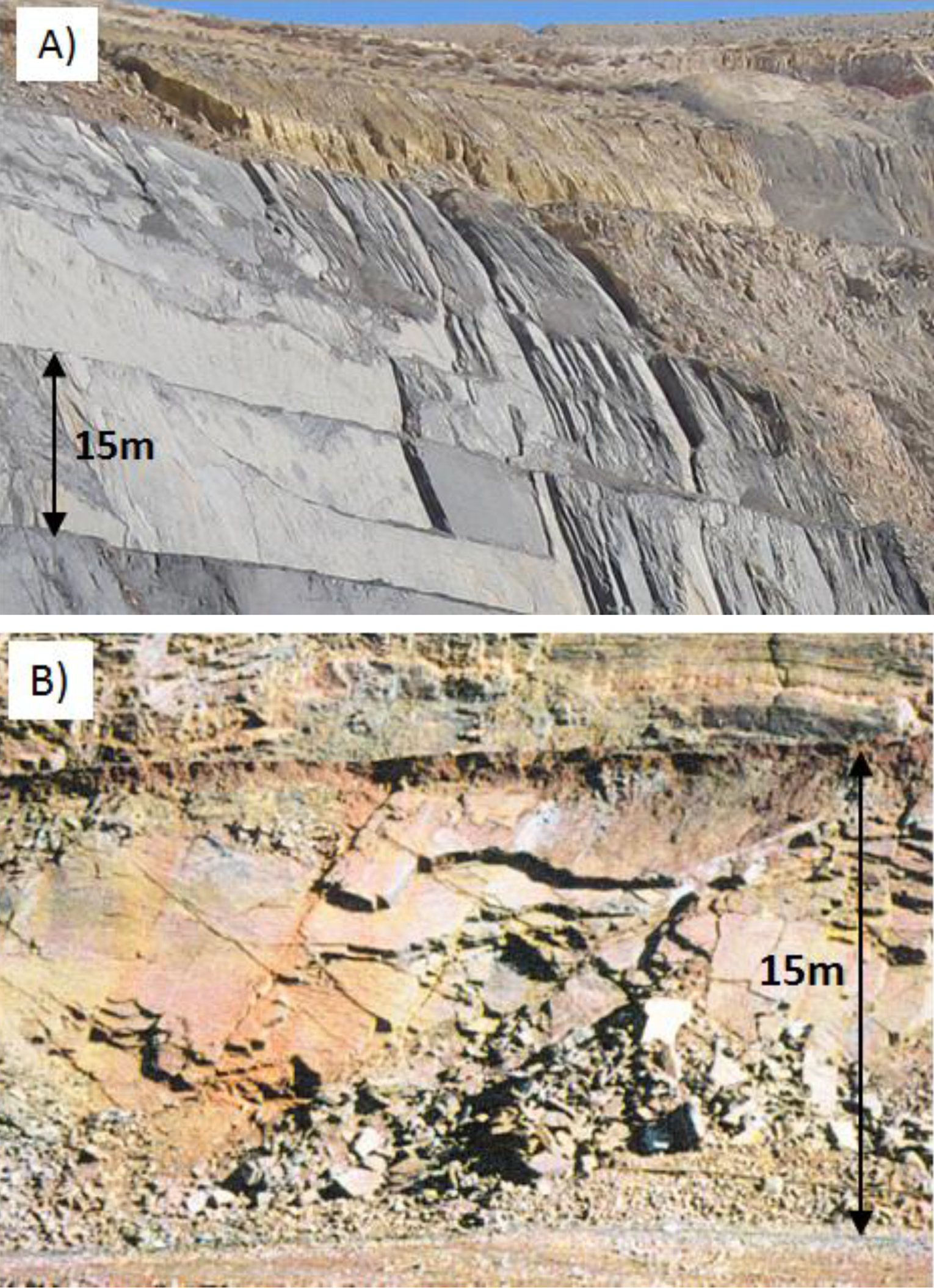
Anisotropic rock masses; a shale and b banded iron formation (Sainsbury and Sainsbury 2013)

When considering anisotropic rock masses, discontinuum analysis techniques provide the most rigorous assessment of the strength and deformation behaviour. In this case, the joint fabric and intact rock are explicitly simulated. However, owing to current computational limitations, it is not possible to explicitly simulate the detailed joint fabric that controls anisotropy in large-scale pit slopes, particularly in three dimensions. Consequently, ubiquitous joint constitutive models are commonly used. The ubiquitous-joint model is an anisotropic plasticity model that includes weak planes of specific orientation embedded in a Mohr–Coulomb solid. Yield may occur in either the solid or along the weak plane, or both, depending on the stress state, the orientation of the weak plane and the material properties of the solid and weak plane. Sainsbury and Sainsbury (2013) developed a methodology for deriving anisotropic rock mass strength using a ubiquitous joint model that closely reproduces 3DEC models that included detailed DFNs (Fig. 12). They used the resultant properties to study the slope stability of a large open-pit mine in Western Australia.

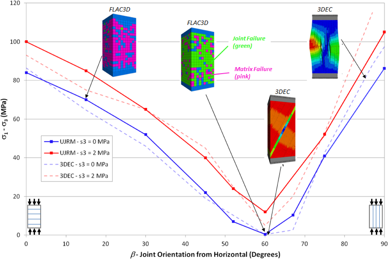
Comparison of 3DEC and FLAC3D – UJRM anisotropic rock mass strength

Kinematic analysis of open pit and underground stability

Simple limit equilibrium method (LEM) techniques that can be used for wedge stability are available in many rock mechanics textbooks (e.g., Brady and Brown 1993). These calculations can be made for individual wedges. Computer software, such as the LEM-based code UNWEDGE, can be used to carry out these calculations efficiently. The software can identify potentially unstable wedge-shaped blocks rapidly for a given excavation shape, orientation and series of joint sets, and calculate the Factor of Safety (FoS) of all potential wedges. The software also can take into account in situ stresses, and can be used for statistical analyses and sensitivity calculations. Finally, the software can account for rockbolt and shotcrete support in the FoS calculation. This is sufficient analysis for many practical problems. In general, the analysis is conservative because discontinuities are assumed to 100% persistent and maximum wedges can occur anywhere. Figure 13 shows an example of the UNWEDGE software.

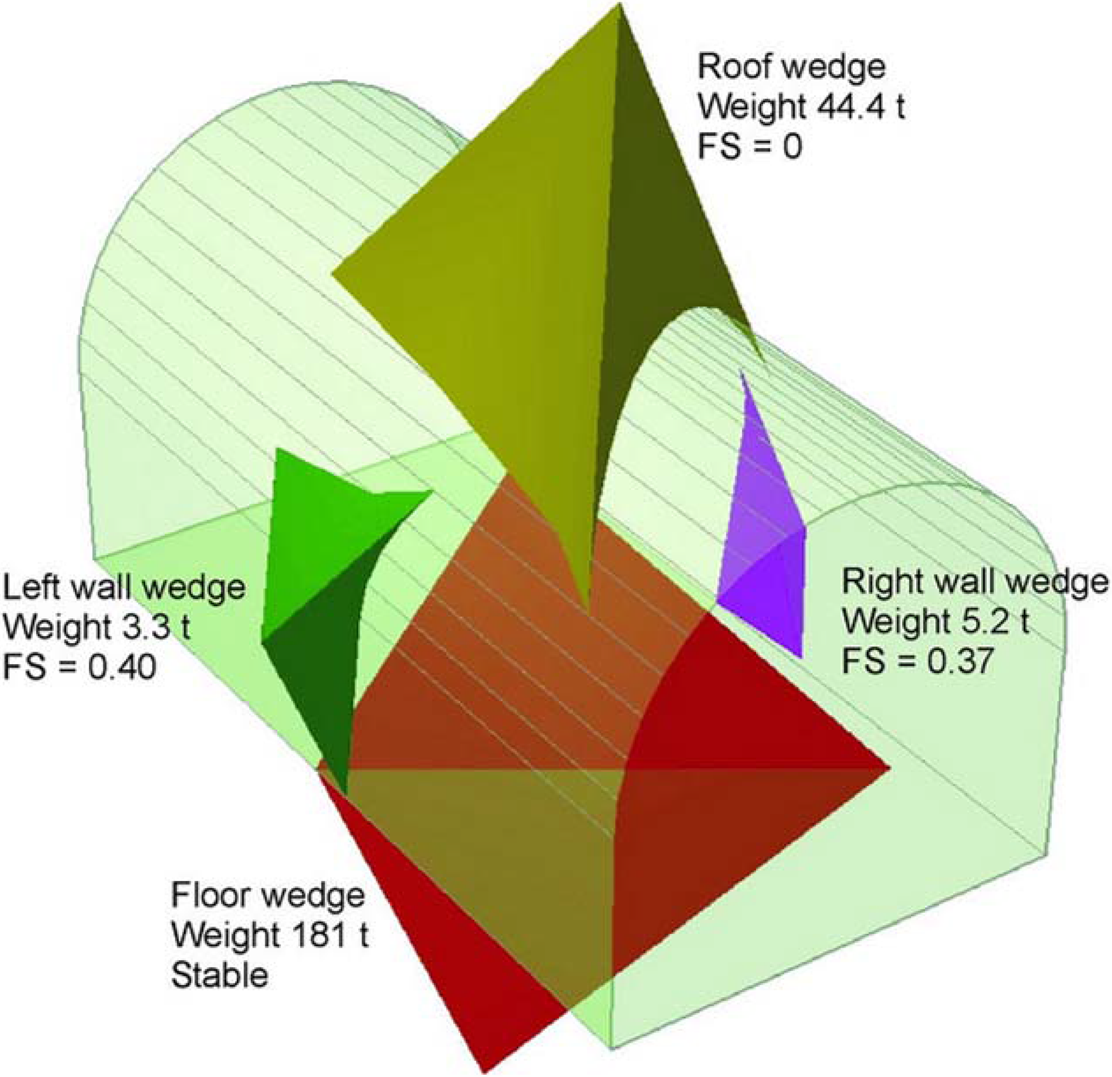
Wedges formed around a tunnel with three joint sets along with LEM-calculated FoS for an unsupported tunnel

More advanced algorithms, e.g., Elmouttie, Poropat and Krähenbühl (2010), utilised by software such as Siromodel allow for the use of all properties associated with a three-dimensional DFN, including the spatial distribution of joints and other structures. The analyses are not limited to statistical representations of these structures, but include representations of the actual structures mapped in the field across (potentially large) exposures. Further, the polyhedral blocks analysed can have unlimited number of faces or shape, therefore accommodating more realistic DFN generation as shown in Fig. 14. One advantage of this approach is that it is sufficiently computationally efficient to allow simulation of numerous DFN realisations and concatenation of the resulting geotechnical analyses. This improves the confidence in estimations of in situ block size distribution, likelihood and spatial distribution of unstable blocks, rock fall analysis and other performance parameters.

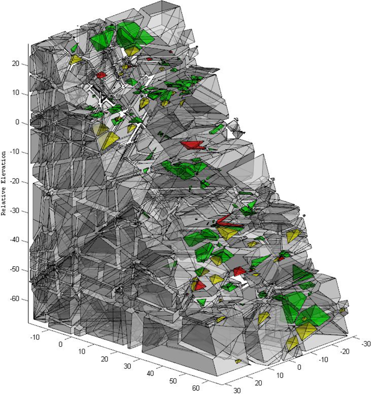
Siromodel analysis of kinematic stability of benches in open-pit mine (Elmouttie, Dean, Krähenbühl and Poropat 2014)

Equivalent porous media models

With regard to the determining of pore pressures in slopes, it is seldom necessary to explicitly model the discrete fracture flow of the entire network of all relevant fractures. More typically, analyses use equivalent porous media (EPM) models with possible explicit inclusion of a few highly permeable discrete structures. EPM models are attractive because they are simple and computationally efficient. Validity of the EPM approximation of the fracture flow is mainly a function of the ratio of the slope height and the typical fracture spacing. Typically, the EPM approach is adequate if the ratio is 25 or greater. This guideline can be used as a first-order approximation, but in general, a methodology based on a directional conductivity graph is preferred. The directional conductivity graph can be used to determine the domain size (or representative element volume, REV) for which the DFN can be approximated by the EPM approximation. Comparison of the REV to the slope size allows the determination of the validity of the EPM assumption. Lorig et al. (2012) showed that in most cases, the errors made by the EPM assumption are small.

Approximation of fracture flow by EPM

Several researchers [e.g., Cundall (1983) and Long (1983)] have used DFN models to determine the conditions for which flow in a rock mass can be modelled as flow in an equivalent continuum. Long and Witherspoon (1985) investigated how the degree of interconnection of fractures affects the magnitude and nature of the permeability of the rock mass. They found that the interconnection of fractures is a function of (1) the fracture density and (2) the fracture size. They varied the density and fracture size in such a way that the fracture frequency (the number of fractures intersecting a borehole) remained constant, and observed that the degree of interconnection increased as the fracture length increased, as later formalised through the percolation parameter concept (see SRM models section). Also, with the increase of fracture length and a corresponding decrease of the fracture density (such that the fracture frequency remained constant), the permeability of the rock mass increased. It is now known that this effect is in fact ‘capped’. There is a limit above which increasing fracture size (at constant density) does not produce any permeability increase (Maillot et al. 2014): the network connectivity is ‘saturated’.

The concept of dimensionless metrics to verify if and when an EPM approach is applicable for fluid flow in fractured media is a well known technique [see for example, Long, Remer, Wilson and Witherspoon (1982); Long and Billaux (1987) and Min (2004)]. The metrics quantify the average error of a porous medium approximation compared to a fully jointed-medium simulation. Lorig et al. (2011) proposed the use of two metrics. The first evaluates the steady-state pressure distribution. The second evaluates the steady-state flow characteristics of a medium – specifically, the directional hydraulic conductivity (see Fig. 15). The metrics quantify the average error of a porous medium approximation compared to a jointed-medium simulation. If a DFN is available for a given site, then the proposed methodology may be used to estimate the magnitude of errors entailed when a porous medium analysis is used.

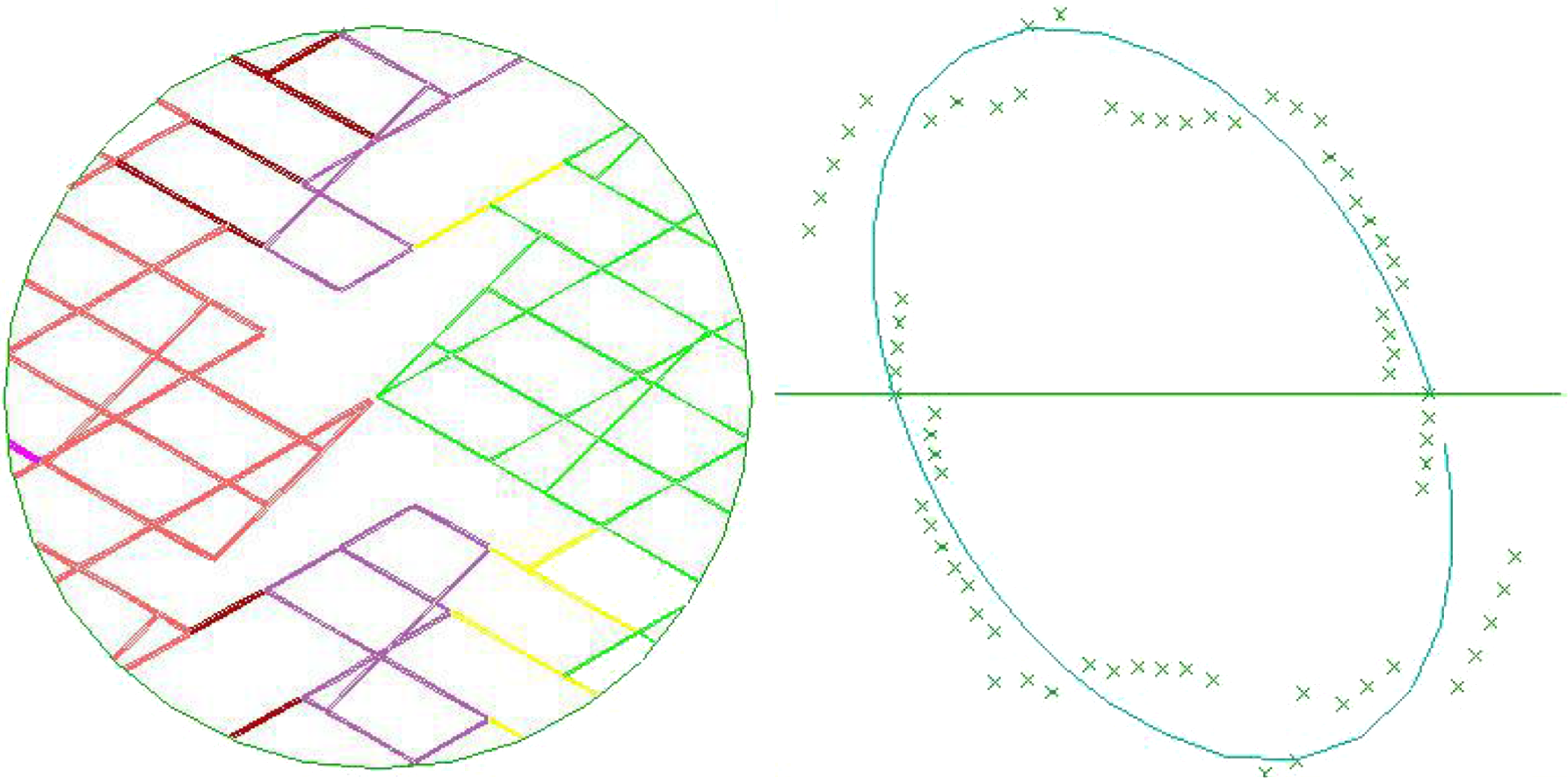
Example of directional permeability graph and ellipse best-fit (right) developed for steady-state flow in discrete fracture network (DFN) (left)

Northwest wall of the Diavik A154 Pit

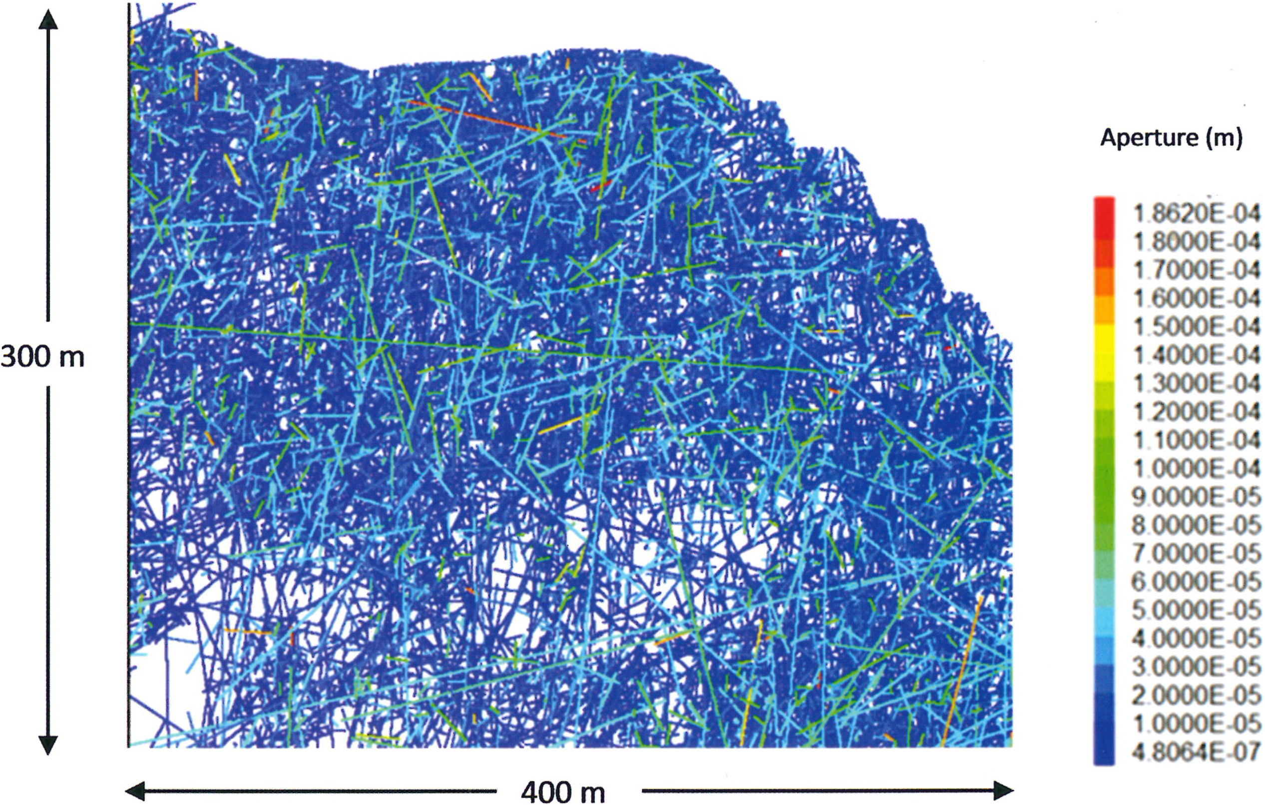
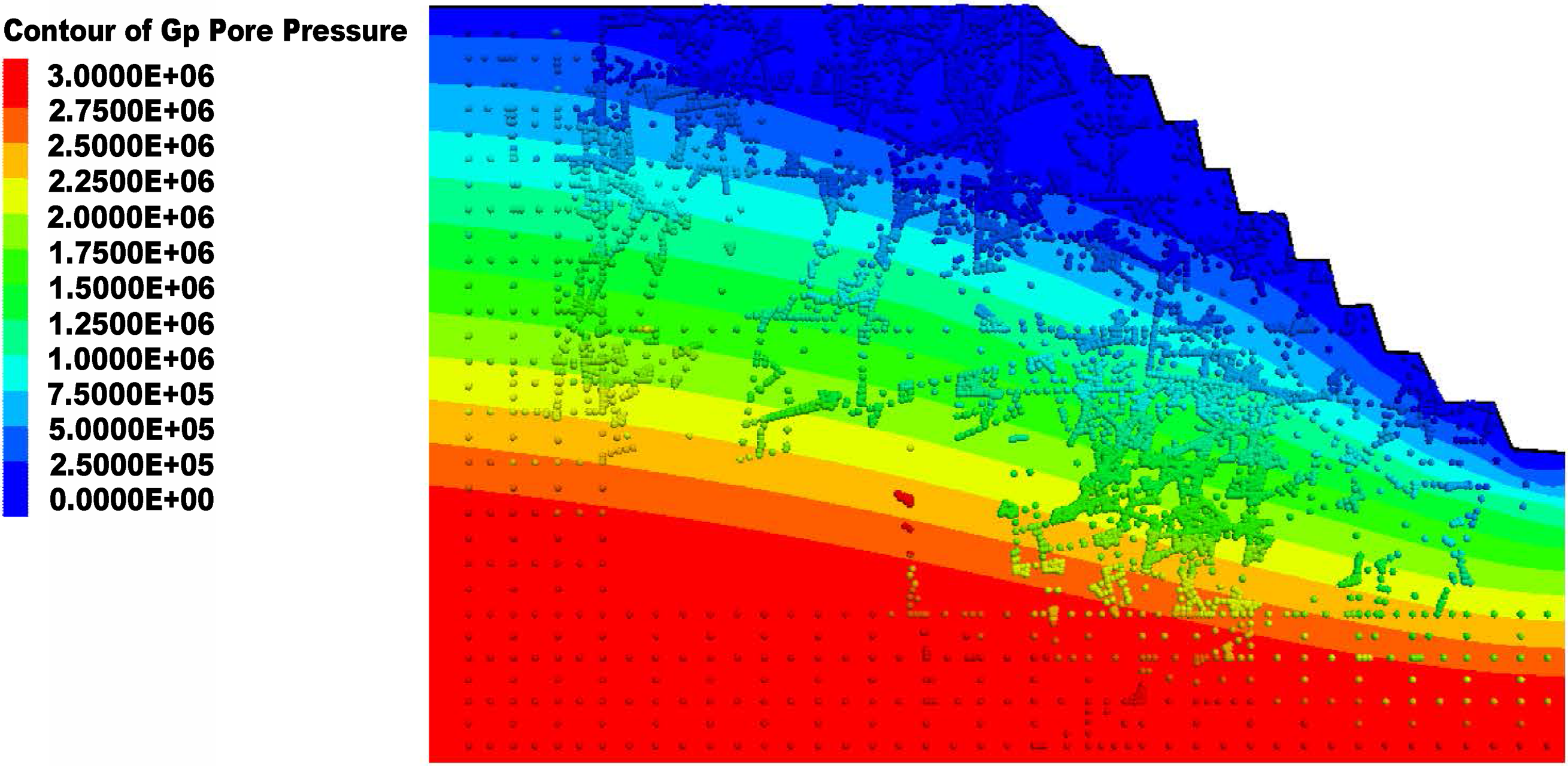
Beale and Read (2014) present a detailed comparison of a DFN-based fracture flow model (see Fig. 16) and an EPM approach for the northwest wall of the Diavik A154 pit (see Fig. 17). Overall, the results of the modelling case study indicated the following.

Similar pore pressure results can be achieved with an EPM model compared with a fracture flow model. The EPM model therefore is considered adequate for simulating pore pressure at the scale and grid size used for the case study.

Close-up of the 2D section of the discrete fracture network (DFN) showing fractures coloured by aperture (Beale and Read 2014)

Pressures from the discrete fracture network (DFN) flow model (dots) superimposed on pressures from the homogeneous equivalent porous media (EPM) model (contours) (pressures are in Pa)

The existence of a DFN model provides a means to define variations in the hydraulic conductivity field by analysing the fracture network. The DFN model also helps provide an understanding of the relative orientation and interaction of the various fracture sets. However, the use of any DFN model as the basis for groundwater flow modelling leads to a major source of uncertainty because of small-scale variations in the transmissivity of different fracture sets and within individual fractures. Use of the DFN method for flow modelling can reveal large variances in predicted parameters (permeability, flow, etc.) depending on the DFN's statistical properties. This is a reflection of the stochastic and epistemic uncertainty associated with the rock mass heterogeneity and the mapping/logging process. The stochastic EPM approach may not be capable of accurately capturing these variances/uncertainties.

Direct evaluation of large-scale slope stability

As shown in SRM models section, DFNs play a fundamental role in the SRM modelling methodology. When setting up the SRM unit, the intact rock properties of the synthetic material are represented by an assemblage of bonded particles calibrated to those measured for an intact sample using a numerical sample size equal to the average intact-block sizes in the slope being analysed. These properties typically include measured values of modulus, Poisson's ratio, UCS, tensile strength and fracture toughness. The joints are represented by a sliding joint model that allows associated particles to slide through, rather than over, one another and, thus, represent joints that can both slide and open in the normal way. The constitutive material properties of the SRM unit itself are not given directly; they result from the response of the combined behaviour of the intact material and included joint fabric when subjected to the likely range of slope-induced stresses. The SRM model for the slope exampled in Fig. 18 is shown in Fig. 19.

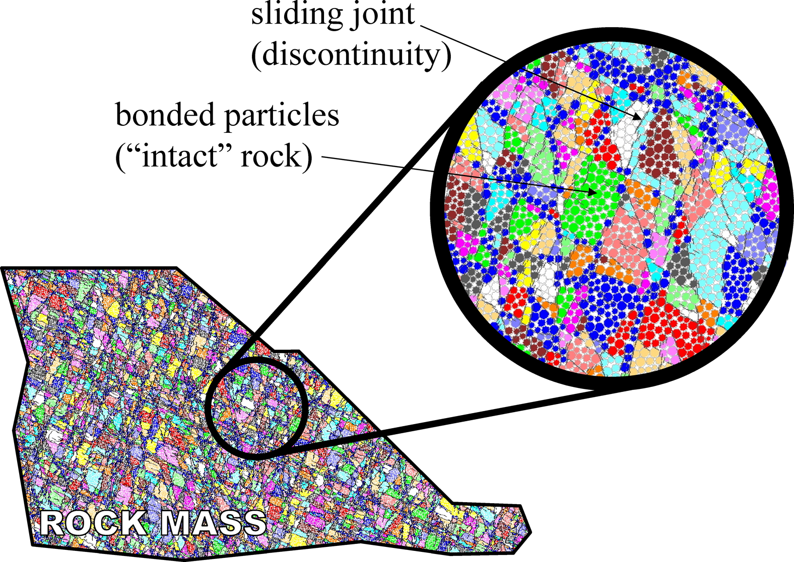
Fully bonded PFC2D model for high slopes in closely jointed rock. Discrete Fracture Network, 500-m high slope

Portion of a discrete fracture network (DFN) network for a 500-m high, 1000-m wide slope intersected by eight persistent fault sets and two joint sets. Colours indicate individual blocks

In the analysis of the slope illustrated in Fig. 18, rock fracture did not occur, but there were considerable yielding and dislocation of the smaller blocks to depths of up to 130 m (Fig. 20) and toppling on the major structures (Fig. 21). Although large-scale rock fracturing did not occur, the toppling and dislocation of the smaller blocks of rock to depths of about 130 m closely resemble the observed behaviour of the slope. It has been suggested that the lack of rock fracture is possibly a 2D artefact in that the intersection of the given fault and joint sets created many discrete blocks or closed areas in 2D. Geometrically, this is artificial because in 3D the discontinuity traces are much less likely to form closed volumes. In 3D simulations of block caving where these limitations are not present, it has been found that rock bridge fracture is widespread and seemingly an essential component in determining the behaviour of the rock mass (Cundall 2008).

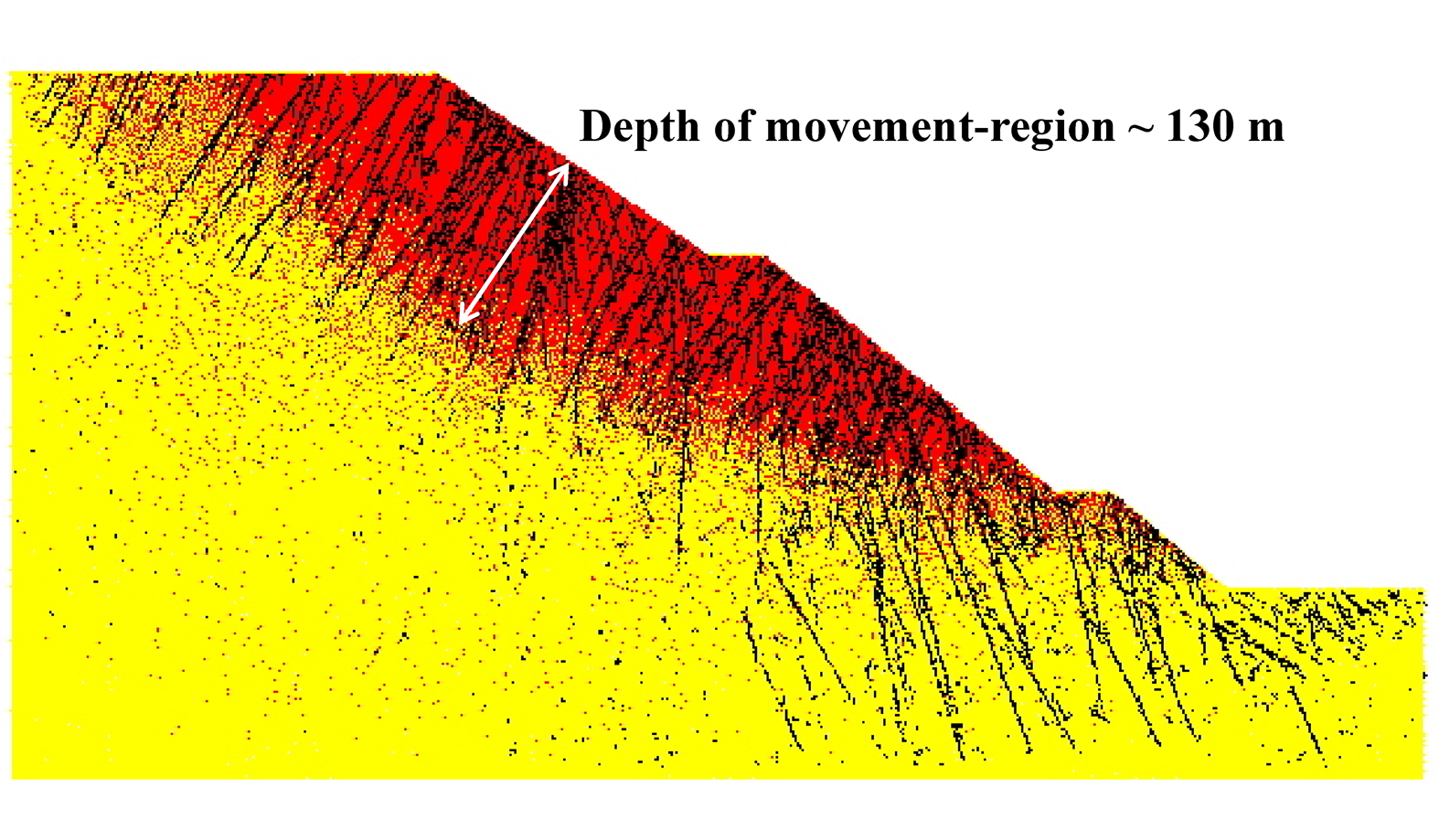
PFC2D model showing area near slope with high velocity (red) overlying shear joints, with yielding and dislocation of smaller blocks to depths of about 130 m (Cundall 2008)

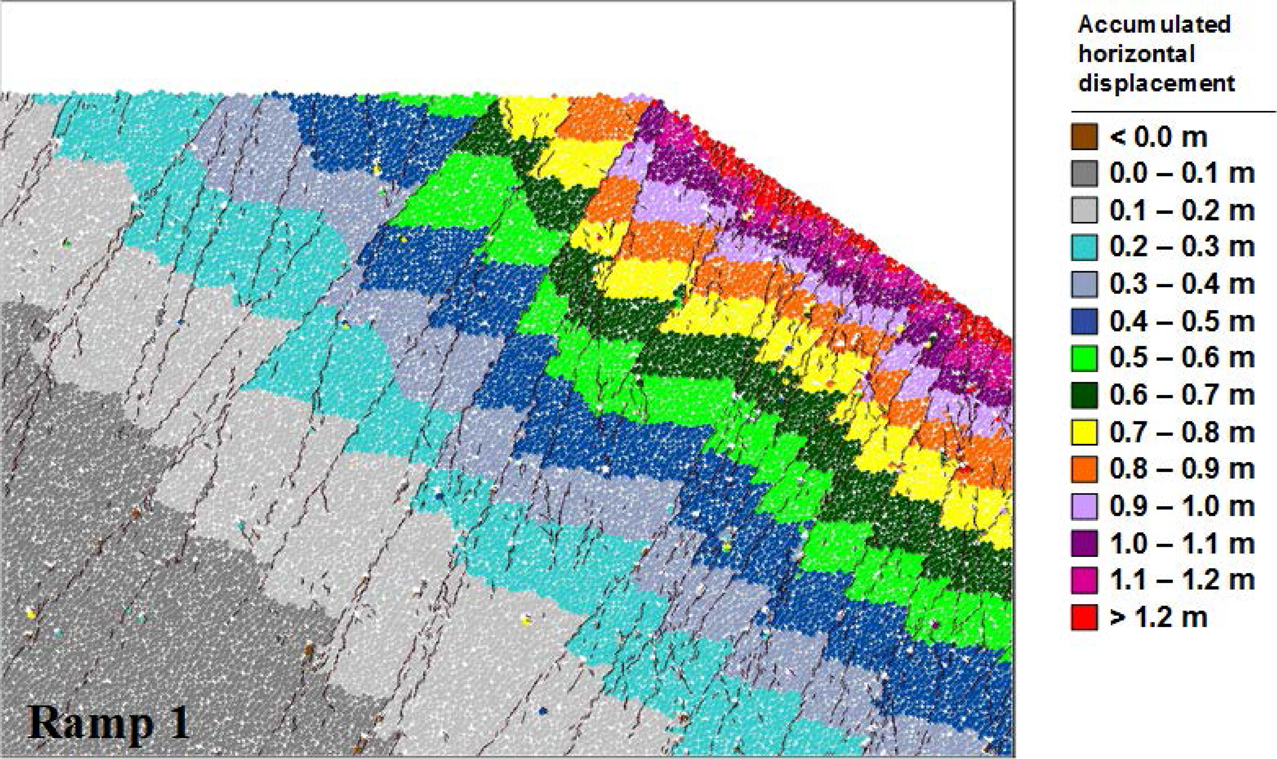
PFC2D model showing toppling on major structures as indicated by discontinuous displacement contours (Cundall 2008)

Most SRM modelling relies on bonded spherical particles to represent the rock mass. Greater efficiency can be realised for brittle rock if a ‘lattice’ consisting of point masses connected by springs replaces the balls and contacts of a typical PFC model. The lattice model still allows fracture by breakage of springs and joint slip by using a modified version of the SJM (smooth joint model) as shown in Fig. 19. The formulation of a new 3D program, Slope Model, based on a lattice representation of brittle rock originally was described by Cundall and Damjanac (2009). The program accepts a general DFN consisting of multiple joint segments that are overlaid on the lattice springs. Fluid flow throughout the jointing network also is modelled with the resulting pressures being used to compute effective stresses (used to assess failure conditions) on each joint element. The influence of deformation on fluid pressure is also explicitly accounted for. Thus, Slope Model can simulate the time evolution of the field of pressures and flows owing to mining activities, and the resulting influence on stability. Example applications can be found in Lorig, Cundall, Damjanac and Emam (2010) (Fig. 22).

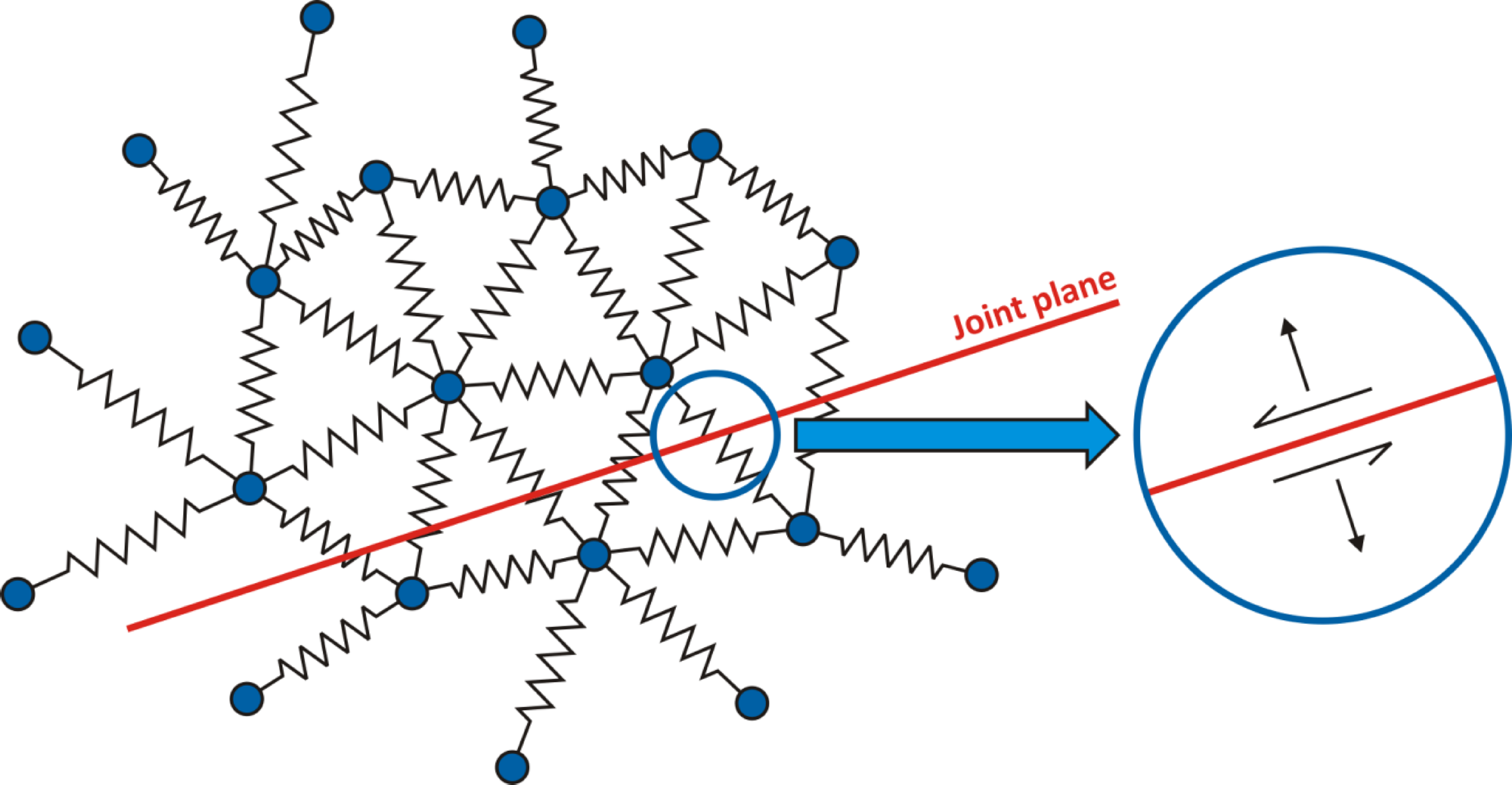
Lattice scheme for a jointed rock mass. Discontinuities are represented by the ‘smooth joint model’ as used in Particle flow code (PFC)

The lattice formulation of Slope Model is similar to that of the HSBM code BloUp (Furtney, Cundall and Chitombo 2009), used for simulating the complete blasting process. In particular, the damage induced in a slope near the blast site can be quantified by BloUp in terms of microcracks (broken lattice springs). It may be possible (in a future development) to import this damage field into Slope Model in order to include the effect of blast damage on slope stability.

Civil engineering (nuclear waste repositories)

Applications of DFNs in civil engineering are perhaps less common than those in mining. However, more DFN-related research has been performed in support of nuclear waste repositories than for mining. This is because flow and transport properties of fractured rock and the associated predictions are of crucial importance for nuclear waste repositories (see, for example, Follin and Hartley (2014) and Follin et al. (2014) and). Although DFNs are important in flow studies, they are also important in excavation stability analyses. Both applications are discussed here.

Flow studies

When the rock matrix can be considered as impermeable, flow occurs by fractures. Then the multi-scale and variable characters of natural fracture systems exert a strong control on fractured rock hydraulic properties. At the same time, access to structure and hydraulic data is severely limited and most fracture systems (except for the largest structures) can be characterised only by means of statistical descriptions (i.e., laws and parameters). Discrete Fracture Network modelling approaches have been largely used to improve the understanding of fractured rock flow structures (Berkowitz 2002).

The determination of fractured rock effective permeability from DFN models follows similar methodologies to those described above for slopes. However, while EPM models provide satisfactory estimates of average water pressure for stability analyses, they generally do not provide good answers to important questions in nuclear waste isolation. Nuclear waste isolation often depends on determining the fastest transport path from the repository to the accessible environment and/or vice-versa. This is a much more difficult problem to solve because it relies on determining flow characteristics at the tails of the distribution (e.g., the most permeable fractures, the highest connectivity, the most persistent structures, etc.). Stochastic analyses of flow channelling may be important in answering these questions. Flow channelling is a striking characteristic of geological systems which appears to be not well represented by Poissonian models.

Directional permeabilities (and ellipse definition) to determine the permeability tensor (and validate the use of equivalent porous medium EPM) is applicable if the considered size (at which permeability is computed) is larger than the REV (Representative Elementary Volume). If the REV is unknown, then the approach should be done for varying scales L (L the size of the spherical domain where permeability is computed for varying directions) and shows there is no evolution of permeability with scale. If there is an evolution of permeability with scale, then the EPM is not easily applicable [see Maillot et al. (2014)]. The REV is potentially not defined (or simply equal to the maximum size of the problem) when the DFN has a multi-scale fracture size distribution like a power law (which is the currently accepted model both in Sweden and in Finland). However, this depends on the balance between fracture sizes, densities and transmissivities. This issue of REV definition is even more critical for nuclear waste studies since the selected sites in principle have as low fracture densities as possible. In addition, a very low proportion of the geological DFN is effectively flowing in these media.

Excavation stability

Lin et al. (2007) studied the behaviour of the tunnels at the Yucca Mountain nuclear waste repository site under in situ, thermal and seismic conditions. A statistically equivalent fracture model was generated based on the extensive underground fracture mapping data. Three-dimensional distinct block analyses were performed using fracture patterns randomly selected from the fracture model.

The blocks of non-lithophysal rock at the site are significantly stronger than the in situ and thermally induced stresses, and thus the problem of modelling this material was essentially one of elastic blocks separated by fracture surfaces. Therefore, in modelling of the stability of the tunnels and the rockfall that may occur from the applied load, the fracture geometry and surface properties are of primary importance. Three-dimensional discontinuum numerical methods are required for correct representation of the degradation mechanism. The approach to modelling mechanical degradation and rockfall from combined in situ, thermal and seismic loading in non-lithophysal rocks is illustrated in Fig. 23. This approach involves modelling of emplacement drifts excavated within the stochastically defined, representative fractured rock mass volume, followed by application of in situ, thermal and seismic load. A large number of parameter studies are conducted in which the tunnel location (and fracture geometry), rock fracture surface properties and loading conditions are varied to derive a conservative range of performance response (in terms of rockfall mass, volume and opening shape) that is indicative of the possible geologic conditions at depth.

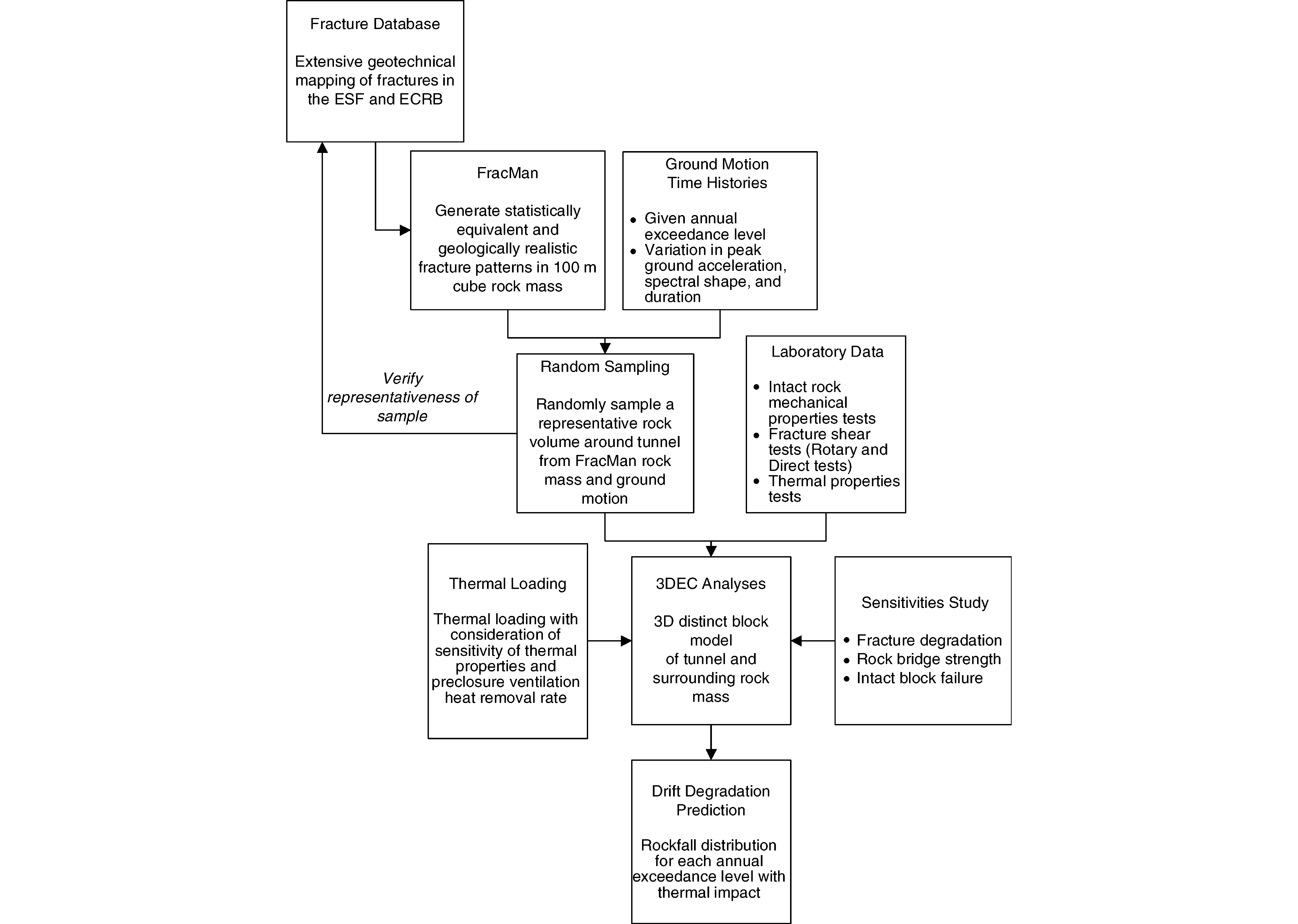
Approach of drift degradation and rockfall analyses (Lin et al. 2007)

The development of a stochastically defined fracture system, representative of the actual rock mass, was performed with FracMan (Dershowitz 1984). The existing fracture mapping database provided the basic input to FracMan, which develops sets of planar, circular fractures that conform to the statistical variability of the geometric characteristics of the input data. Statistical models are fitted to the various geometric characteristics of each fracture set in the database, followed by generation of representative fracture sets. These representative fractures then are back-checked against the statistical variability and geologic realism of the field data to achieve an acceptable facsimile. A three-dimensional representative rock mass cube, 100 m on a side, was generated using FracMan and composed of the matrix blocks defined by approximately 90 000 fractures. Each fracture is described by its centroid coordinate, dip, dip direction and radius. These geometric properties are used as direct inputs to 3DEC for development of a block geometry within which emplacement drifts can be randomly excavated.

The three-dimensional depiction of an emplacement drift after seismic shaking provides a physical perspective for the impact of seismically induced rockfall on drift profile. Figure 24 shows the rockfall profile for the case showing the greatest amount of rockfall with 10^− 6 (i.e., once in a million years) hazard level earthquake.

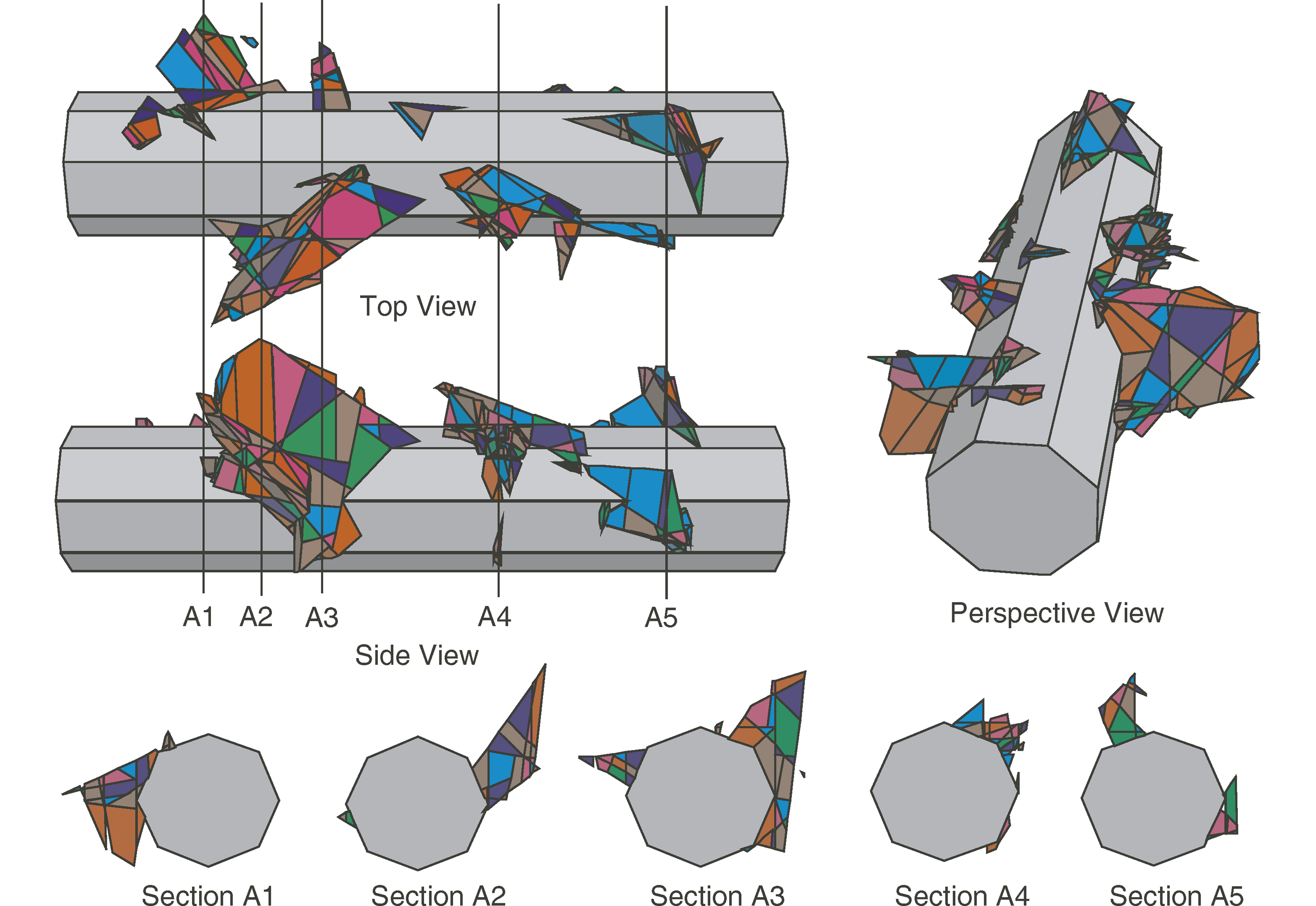
Predicted maximum Rockfall for 1 × 10^− 6 Hazard Level earthquake (Lin et al. 2007)

Challenges

Because of the difficulty to characterise the complex and multi-scale nature of DFN systems (Davy et al. 2010; Bonnet et al. 2001; Davy, Le Goc and Darcel 2013; Fox, La Pointe, Hermanson and Öhman 2007), DFN applications are still facing challenging issues, such as what is the appropriate conceptual DFN model that captures the physics of a problem, and how does that DFN depend on the type and scale of the given problem? Are the current numerical modelling capacities sufficient to model this complexity? This imposes limits to the level of detail that can be modelled.

Application of DFNs in mining and civil engineering therefore face important challenges in two areas: validation and simplification. These two areas overlap to some extent, but it seems logical to discuss validation first, and then simplification.

DFN validation

In spite of the fact that DFN models have been available for several years, there are still questions about their overall reliability and whether inaccuracies in the DFN model could give rise to significant errors in the overall SRM model, for example.

A number of tools have been developed in the past for managing DFN data and building DFN numerical models. Acquisition methods are constantly improving and allow for increase in the amount of accurate data. For example, coupling JKJointStats and SiroVision enables efficient geometrical characterisation of the fracture traces on the face of an open pit. These software tools produce networks from statistical properties, or may help assess the statistical properties, given a conceptual model.

In most cases, access to a fully deterministic representation of a fractured system is simply impossible. Therefore, in practice the DFNs are characterised by means of statistical distributions and models (Fox et al. 2007; Darcel et al. 2013a, 2013b). The access to data in order to characterise DFN models is limited in most cases by strong constraints. First, observations are limited in dimension; scanline mapping, core logging, tunnel wall or outcrop mapping provide partial 1D or 2D observations of the real fracture system, which is 3D. The parent 3D distribution model is built by means of stereological rules to account for these biased observations. Observations also are limited in terms of scale and quantity. The sampling scale may be different from the application scale, and the amount of data appears scarce with regard to the size of the given problem. Despite the addition of geological information and flow data (for flow applications), available information is insufficient to uniquely characterise DFN models, and modelling assumptions are necessary to perform modelling calibrations. Overall, modelling uncertainties not only stem from the estimation of parameters that may be performed by these tools, but also from the (less than perfect) adequacy of the conceptual model. Assessing this adequacy and the relevance of the given model for a specific problem is still an open fundamental issue. Scaling (fracture sizes), spatial variability and spatial correlations (including intersections and termination) are of critical importance (Le Goc et al. 2014; Davy, Le Goc and Darcel 2014). All these aspects influence the resulting mechanical behaviour, from SRM-scale testing to cavescale modelling. This research work, which is important for assessing and improving the reliability of DFN modelling, is continuing.

Finally, beyond the DFN scale issue, the fracture scale and fracture properties raise many issues. Dreuzy et al. (Dreuzy, Méheust and Pichot 2012) shows in a fundamental approach how fracture-scale heterogeneities affect the network scale behaviour. Hoek and Martin (2010) raise the challenging difficulty to distinguish between fractures that are open, tight or sealed. It is difficult to identify practically open and sealed joints from rock core, televiewer logs and rock outcrops with any degree of confidence. The sampling and/or blasting process disturbs all core/outcrop samples. Hence, separating open fractures from sealed fractures is particularly challenging.

Hydrogeologists overcome this issue by calibrating their DFN to groundwater flow and head measurements. Since only open connected fractures conduct flow, this is a practical way to calibrate the DFN. However, there is no such practical approach for calibrating a DFN model for mechanical analyses. Thus, it is difficult to assess if the mechanical model results that utilise a DFN are more realistic or not.

DFN simplification

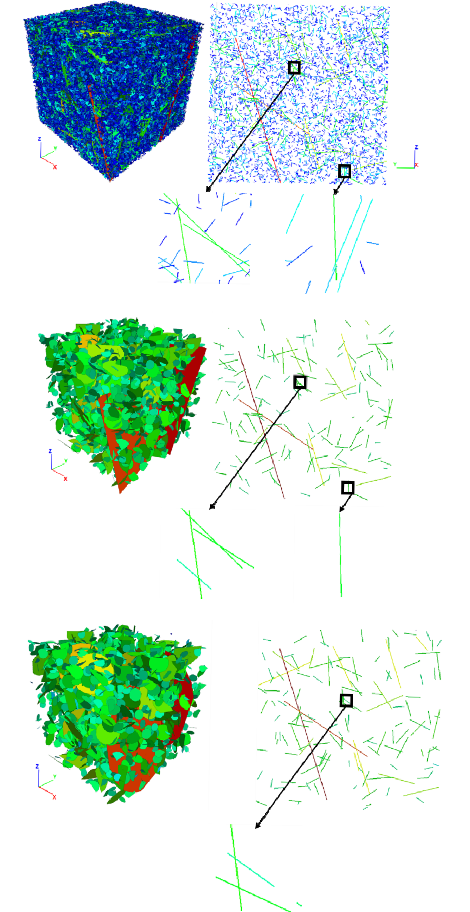
DFN models define the statistical distributions of fracture geometrical characteristics such as the fracture size, orientation and density distributions. A widely used definition of fracture positions is the random Poisson process in which nothing prevents any two fractures from falling in the close proximity of each other. In such a model, thousands of fractures can exist and particular configurations such as those illustrated in Figure 25a are common. Rock bridges can vanish locally, become very thin or create low-angle intersections. These configurations may occur even with very few fractures, and increase quickly with the fracture density. Therefore, local rock bridge resolution is potentially the source of numerical difficulties such as severe computational time increases or accuracy degradation. Local configurations are thus, along with the large number of fractures required to properly model the natural complexity, a strong limiting factor for the integration of DFNs in numerical models and require further study. Itasca is investigating the following practical avenue as a way to address the issue. (1)

Define what combination of fracture sizes, rock bridge size and model refinement (particle or zone size) are acceptable (Fig. 25a).

(2)

Optimise and simplify DFN to remove issues while preserving its relevant properties. The simplest modification consists of removing fractures while updating the ‘intact rock’ effective properties accordingly. Figure 25b illustrates a typical practice: removal of small fractures. A more complex one consists of somehow replacing the configuration by an acceptable equivalent that would not create numerical issues. In a preliminary version of this step, pairs of fractures with close orientations and locations are identified and merged (Fig. 25c).

a 3D discrete fracture network (DFN) and partial 2D cut view of a complex DFN (L = 100, lmin = 1, a = 4, p = 6) with insight to potential local critical configurations; b same DFN where fractures with l < 5 are removed; c same DFN as b, but with fracture combination

In both cases, consequences of the adaptation and resulting potential alteration of mechanical and DFN connectivity properties will be assessed.

Conclusions

Discrete Fracture Networks in mining and civil engineering have been used to significant advantage in a variety of ways. In mining engineering, DFNs have been fundamental in the development of the SRM model for mechanical analyses. The current state of SRMs is summarised by Hoek, Carter and Diederichs (2013):

Numerical techniques such as the Synthetic Rock Mass model (Mas Ivars et al. 2011) provide the means of incorporating the joint fabric of a rock mass at different scales. In the long run, these methods have the potential to allow direct three-dimensional modeling of all of the physical components of a rock mass and provide a much more rigorous alternative to the empirical characterization and rock-mass parameter estimation approach using the GSI chart. In the short term, numerical modeling techniques can be used to develop rock structure scales that incorporate both the scale of the rock blocks and the scale of the engineering structure in which they exist.

Hoek and Martin (2010) argue that the best way to validate a DFN is to measure parameters that depend on the DFN description. In hydrogeology, the measured parameters head and flow can be calibrated to a DFN. However, there are no such parameters for mechanics. Therefore, the DFN in mechanical analyses cannot be evaluated directly, which is a significant shortcoming. Before the popularity of the DFN, joint mapping along underground openings was used to describe the formation of wedges to estimate support. However, it can be demonstrated that jointing described in a ubiquitous manner significantly overestimates the spatial distribution and size of wedges that can form. Hence, it remains a significant challenge to utilise the characteristics of a DFN in a meaningful manner. Linking a DFN to a hydrogeological model should improve the characteristics of the DFN to provide a meaningful description of the rock mass fractures.

Acknowledgements

Slope Model was developed under a collaborative research agreement with the CSIRO in Brisbane, QLD, Australia as part of the Large Open Pit (LOP) Project. The use of DFNs in caving studies was developed under a collaborative research agreement with the Sustainable Mining Institute (SMI) as part of the Mass Mining Technology (MMT) project. The Sponsors of both projects are thanked for their support. SKB is also thanked for its support on research about DFN modelling framework. Input from Marc Elmouttie (CSIRO) in SRM models section is also gratefully acknowledged.This paper was originally presented at the first International Conference on Discrete Fracture Engineering (DFNE 2014) (19–22 October 2014, Vancouver, BC, Canada) and has subsequently been revised before consideration by Mining Technology.

References

Barton

2000. TBM tunneling in jointed and faulted rock, Rotterdam, Balkema.

Beale

and Read

2014. Guidelines for evaluating water in pit slope stability, Collingwood, CSIRO Publishing.

Berkowitz

2002. Characterizing flow and transport in fractured geological media: a review, Advances in Water Resources, 25, (8-12), 861–884.

Bonnet

, Bour

, Odling

N. E.

, Davy

, Main

, Cowie

and Berkowitz

2001. Scaling of fracture systems in geological media, Reviews of Geophysics, 39, (3), 347–383.

Bour

and Davy

1998. On the connectivity of three-dimensional fault networks, Water Resources Research, 34, 2611–2622.

Brady

B. H.

and Brown

E. T.

1993. Rock mechanics for underground mining, 2nd edn., New York, Chapman & Hall.

Carvalho

J. L.

, Kennard

D. T.

and Lorig

2002. Numerical analysis of the east wall of Toquepala Mine, Southern Andes of Peru, in Proceedings of EUROCK 2002, (eds. Dinas da Gama

and Ribeiro e Sousa

., 615–625, Lisbon, Sociedade Portuguesa de Geotecnica.

Clark

I. H.

2006. Simulation of rock mass strength using ubiquitous joints, in Proceedings of the Fourth International FLAC Symposium on Numerical Modeling in Geomechanics, (eds. Hart

and Varona

., Minneapolis, Itasca Consulting Group, Inc.. [Paper No. 08-07].

Cundall

2008. Recent advances in numerical modelling for large-scale mining projects, ACG Newsletter, 30, 1–7.

10.

Cundall

P. A.

1983. Numerical modelling of water flow in rock masses. Report No. DOE/RW/83.059, Technical Report to Geognosis, United Kingdom DOE.

11.

Cundall

P. A.

and Damjanac

2009. A comprehensive 3D model for rock slopes based on micromechanics, in Slope Stability 2009. Santiago, November 2009, Chile, Universidad de Los Andes.

12.

Damjanac

, Gil

, Pierce

and Sanchez

2010. A New approach to hydraulic fracturing modeling in naturally fractured reservoirs, in Proceedings of the 44th U.S. Rock Mechanics Symposium. Alexandria, Virginia: ARMA. [Paper No. 10-400].

13.

Darcel

, Davy

and Le Goc

2013a. Development of the statistical fracture domain methodology: application to the Forsmark site. SKB R-13-54, Stockholm, Svensk Kärnbränslehantering AB (SKB).

14.

Darcel

, Le Goc

and Davy

2013b. The elastic properties of fractured rock, in AGU Fall meeting, San Fransisco, AGU.

15.

Davy

, Le Goc

and Darcel

2013. A model of fracture nucleation, growth and arrest, and consequences for fracture density and scaling, Journal of Geophysical Research Solid Earth, 118, (4), 1393–1407.

16.

Davy

, Le Goc

and Darcel

2014. A non-Poissonian, likely-universal, fracture model for hardrock DFN, in Proceedings of the First International Conference on Discrete Fracture Network Engineering. Vancouver.

17.

Davy

, Le Goc

, Darcel

, Bour

, de Dreuzy

J. R.

and Munier

2010. A likely-universal model of fracture scaling and its consequence for crustal hydro-mechanics, Journal of Geophysical Research Solid Earth, 115, B10411.

18.

Dershowitz

W. S.

1984. Rock joint systems. PhD Thesis, Massachusetts Institute of Technology, Massachusetts.

19.

Dreuzy

J. R.

, Méheust

and Pichot

2012. Influence of fracture scale heterogeneity on the flow properties of three-dimensional discrete fracture networks (DFN), Journal of Geophysical Research: Solid Earth, 117, B11.

20.

Elmouttie

, Dean

, Krähenbühl

and Poropat

2014. Structural mapping and analysis for open pits. CSIRO Earth Science and Resource Engineering, Presentation, April.

21.

Elmouttie

, Poropat

and Krähenbühl

2010. Polyhedral modelling of underground excavations, Computers and Geotechnics, 37, 529–535.

22.

Follin

and Hartley

2014. Approaches to confirmatory testing of a groundwater flow model for sparsely fractured crystalline rock, exemplified by data from the proposed high-level nuclear waste repository site at Forsmark, Sweden, Hydrogeology Journal., 22, (2), 333–349.

23.

Follin

, Hartley

, Rhen

, Jackson

, Joyce

, Roberts

and Swift

2014. A methodology to constrain the parameters of a hydrogeological discrete fracture network model for sparsely fractured crystalline rock, exemplified by data from the proposed high-level nuclear waste repository site at Forsmark, Sweden, Hydrogeology Journal., 22, (2), 313–331.

24.

Fox

, La Pointe

, Hermanson

and Öhman

2007. Statistical geological discrete fracture network model, Forsmark modelling stage 2.2, Sweden, Svensk Kärnbränslehantering AB.

25.

Furtney

J. K.

, Cundall

P. A.

and Chitombo

G. P.

2009. Developments in numerical modeling of blast induced rock fragmentation: updates from the HSBM Project, in Proceedings of rock fragmentation by blasting, (ed. Sanchidrián

J. A.

., 335–342, London, CRC Press/Taylor & Francis Group.

26.

Hoek

2004. Estimates of rock mass strength and deformation modulus, Rocscience. Available at: < http://www.rocscience.com/library>. [Discussion Paper No. 4].

27.

Hoek

and Martin

2010. Synthetic Rock Mass Review, Report to MMT2, Queensland, The Sustainable Minerals Institute, University of Queensland.

28.

Hoek

, Carter

T. G.

and Diederichs

M. S.

2013. Quantification of the Geological Strength Index chart, in Proceedings of the 47th US Rock Mechanics/Geomechanics Symposium. ARMA13-672, San Francisco, California: ARMA.

29.

Itasca Consulting Group, Inc.. 2004. UDEC – universal distinct element code, Ver. 4.0 user's manual, Minneapolis, Itasca.

30.

Itasca Consulting Group, Inc.. 2011. FLAC – fast Lagrangian analysis of continua, Ver. 7.0, Minneapolis, Itasca.

31.

Itasca Consulting Group, Inc.. 2012. FLAC3D – fast Lagrangian analysis of continua in three-dimensions, Ver. 5.0., Minneapolis, Itasca.

32.

Itasca Consulting Group, Inc.. 2014. PFC – particle flow code, Ver. 5.0, Minneapolis, Itasca.

33.

Kachanov

1987. Elastic solids with many cracks, a simple method of analysis, International Journal of Solids and Structures, 23, (1), 23–43.

34.

Kachanov

and Laures

J. P.

1989. Three-dimensional problems of strongly interacting arbitrarily located penny shaped cracks, International Journal of Fracture, 41, (4), 289–313.

35.

Le Goc

, Darcel

, Davy

, Pierce

and Brossault

M. A.

2014. Effective elastic properties of 3D fractured systems. Proceedings of the First International Conference on Discrete Fracture Network Engineering, Vancouver.

36.

Lin

, Damjanac

, Board

, Kicker

and Leem

2007. Mechanical degradation of emplacement drifts at yucca mountain - a modeling case study, part II: lithophysal rock, International Journal of Rock Mechanics and Mining Sciences, 44, 368–399.

37.

Long

J. C.

and Billaux

1987. From field data to fracture network modeling, Wat. Resources Res., 23, (7), 1201–1216.

38.

Long

J. C. S.

1983. Investigation of equivalent porous medium permeability in networks of discontinuous fractures. PhD Thesis, University of California, Berkeley.

39.

Long

J. C. S.

and Witherspoon

P. A.

1985. The relationship of the degree of interconnection to permeability in fracture networks, Journal of Geophysical Research, 90, 3087–3098.

40.

Long

J. C. S.

, Remer

J. S.

, Wilson

C. R.

and Witherspoon

P. A.

1982. Porous media equivalents for networks of discontinuous fractures, Water Resources Research, 18, (3), 645–658.

41.

Lorig

, Cundall

P. A.

, Damjanac

and Emam

2010. A Three-dimensional model for rock slopes based on micromechanics, in Proceedings of the 44th U.S. Rock Mechanics Symposium and 5th U.S.-Canada Rock Mechanics Symposium. Alexandria, Virginia: ARMA, 2010. [Paper No. 10-163].

42.

Lorig

, Damjanac

, Detournay

, Hazzard

, Riahi

and Cundall

2011. Assessment of the effect of water pressures on the stability of closely jointed rock, ICG11-2462-24- 49R. Report to CSIRO, Minneapolis, Itasca Consulting Group, Inc.

43.

Maillot

, Davy

, de Dreuzy

J. -R.

, Le Goc

, Darcel

and Stigsson

2014. Comparison between “Poissonian” and “mechanically-oriented” DFN models for the prediction of permeability and flow channeling, in Proceedings of the First International Conference on Discrete Fracture Network Engineering. Vancouver.

44.

Mas Ivars

, Pierce

M. E.

, Darcel

, Montes

J. R.

, Potyondy

D. O.

, Young

R. P.

and Cundall

P. A.

2011. The synthetic rock mass approach for jointed rock mass modeling, International Journal of Rock Mechanics and Mining Science, 48, (2), 219–244.

45.

Min

K. -B.

2004. Fractured rock masses as equivalent continua – A numerical study. PhD Thesis. KTH Land and Water Resources Engineering, Stockholm, Sweden.

46.

Park

E. -S.

, Martin

C. D.

and Christiansson

2004. Numerical simulation of the mechanical behavior of discontinuous rock masses, in Proceedings of the Numerical modeling in micromechanics via particle methods – 2004: International PFC Symposium, (eds. Shimizu

, ). 85–91, Leiden, Balkema.

47.

Reyes-Montes

J. M.

, Pettitt

W. S.

and Young

R. P.

2007. Validation of a Synthetic Rock Mass model using excavation induced microseismicity, in Proceedings of Rock Mechanics: Meeting Society's Challenges and Demands, (eds. Eberhardt

, ). Vol. 1, 365–369, London, Taylor & Francis Group.

48.

Sainsbury

B. -A.

and Sainsbury

2013. Three-dimensional analysis of pit slope stability in anisotropic rock masses, in Proceedings of the 2013 International Symposium on Slope Stability in Open Pit Mining and Civil Engineering, Perth, Australia, ACG (ed. Dight

., 683–696.