Modelling of polymer fluid flow and residence time distribution in twin screw extruder using fictitious domain method

Abstract

The flow behaviour of a polymer melt in the conveying region of an intermeshing corotating twin screw extruder was studied using the combination of mixed finite element and fictitious domain method. The model was a combination of the governing equations of continuity and momentum with Carreau rheological model in a three-dimensional Cartesian coordinate system. The equations were solved by the use of a mixed Galerkin finite element technique. The Picard's iterative procedure was used to handle the non-linear nature of the derived equations. The particle tracking technique was used to obtain residence time distribution and analyse distributive mixing in conveying region. The shear rate distribution was investigated as a criterion for dispersive mixing. The applicability of this model was verified by the comparison of experimentally measured pressure and simulation results for high density polyethylene melt. This comparison shows that there is a good adequacy between experimental data and model predictions.

Keywords

Twin screw extruder Simulation Finite element method Fictitious domain method Residence time distribution

Introduction

Intermeshing corotating twin screw extruders (TSEs) are widely used in polymer industries to achieve intensive mixing, compounding, devolatilisation and also reactive extrusion.1^–4 The theory of the flow in TSEs has not been well developed yet compared to single screw extruders. The main features of this process that prevent researchers from developing a comprehensive and complete flow analysis are:

existence of a complex three-dimensional (3D) flow pattern

ii.

unsteady and non-isothermal flow regime

iii.

partially filled flow domain in conjunction with random free surfaces in the channels

iv.

moving boundaries that changes the shape of the channels continuously.

There are several parameters in TSEs, such as screw configuration and geometry, rotational speed, temperature and feeding rate that affect the operating conditions of these machines. Therefore, it is difficult to adjust them for optimisation of an especial compounding, blending and/or reactive extrusion process. Computer simulation is now being widely used as an important and robust method for the optimisation of the extrusion process.2^–4 There are two approaches used for the numerical study of the flow in TSEs. In the first approach that has been used by Fukuka et al., 5, 6 the geometry was simplified and the model was developed in a 2D framework. The governing equations were then solved for unwrapped channels. Ignoring the complex 3D flow domain and also the moving of the screws in the barrel are the main drawbacks of this method. Therefore, some researchers7^–17 have tried to take the complex 3D geometry and flow domain into account. So far, two methods have been developed for 3D simulation of polymeric fluids in TSEs using the finite element method (FEM). The first method is based on the use of quasi-steady state method. In this method, due to the time dependent flow boundaries, several sequential geometries are created to demonstrate a complete screw rotation cycle. For example, the works carried out by Manas-Zloczower et al., 7, 8 Lawal et al., 9 Mours et al., 10 Ishikawa et al.11 and Bravo et al.12 are all based on the assumption of quasi-steady state. Although this method does not ignore the complexity of the flow domain, the interrelation of the field variables (pressure, velocity and/or temperature) between two consecutive steps still remain unaddressed. This may generate errors in results especially at higher screw rotational speeds. In addition, it requires remeshing at every time step which reduces the applicability of the method. On the other hand, the traditional Lagrangian approach cannot cope correctly with highly deformable flow field in the screw channel. Therefore, the second method is based on the combination of the flow solution method with an additional algorithm that should take the geometry changes into consideration. Among the various methods that were developed based on this strategy, the arbitrary Lagrangian–Eulerian (ALE) and fictitious domain methods are two more common techniques which have extensively used for the modelling of the flow with varying moving boundaries.18, 19 Arbitrary Lagrangian–Eulerian needs a uniform mesh with constant number of nodes and elements to be maintained during the flow analysis. This may prevent its applicability especially when dealing with complex 3D domain such as TSEs. To override this weakness of the ALE method, the fictitious domain method was developed. This method was used by Glowsinki et al.20^–22 and Bertrand et al.23 for the calculation of flow fields and then was further developed by Bertrand et al.24 for the modelling of flow in TSEs. In this method a static mesh for the volume delimited by barrel and a dynamic mesh for screw were selected and at each time step the position of dynamic mesh was updated according to the screw speed.

A literature survey shows that mixing (distributive and dispersive mixing) in TSEs can be evaluated based on the simulated flow fields. There are different parameters that can be used for this purpose such as shear strain, shear rate, shear stress, elongational flow and residence time distribution (RTD).1, 2, 7, 8, 11, 13^–15 The elongational flows are more effective than simple shear flows on dispersive mixing.16 To investigate this phenomenon, Manas-Zloczower et al.7, 8 have introduced a parameter called λ for the quantification of the elongational and shear flow components. The calculation of this parameter from velocity field computed in this work will later be presented in the ‘Results and discussion’ section. Lawal et al.17 analysed theoretically the extensive mixing characteristic of TSEs based on study of striation thickness using FEM. Kruijt et al.25 analysed distributive mixing in TSEs using the mapping method. They calculated the scale of segregation as a parameter of mixing in TSEs. Bravo et al.13 used particle tracking technique to obtain residence times and analyse distributive mixing in kneading elements of corotating a TSE based on the quasi-steady state method.

In this work, a combination of fictitious domain method and mixed FEM has been used for simulation of the polymeric fluid flow in conveying region of corotating TSEs involving moving screws. Using the predicted flow fields, the RTD was calculated based on particle tracking technique to evaluate the distributive mixing in the conveying region of the TSE. Also, the shear rate distribution and its unevenness in the flow field were used for investigation of the dispersive mixing efficiency in the TSE. The mathematical model was developed for the solutions of continuity and momentum equations in 3D Cartesian framework. The well known Carreau model was also used to reflect the rheological behaviour of polymer melt. The main assumptions made in the development of the present models are:

the flow of polymer is laminar and the fluid is incompressible

ii.

the flow is considered to be 3D in Cartesian framework

iii.

body forces are negligible

iv.

the flow regime is isothermal

the channels of the TSE are fully filled.

To examine the validity of the simulation results, the pressure of high density polyethylene (HDPE) melt has been measured in the TSE (fully filled region) and compared with the theoretically predicted values. In the following sections, we first describe the mathematical model and then the numerical strategy is introduced. The simulation results and comparison of those with experimental results are presented in the next section and finally conclusions are drawn.

Mathematical model

Fluid phase

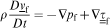
The governing equations of the flow of an incompressible generalised Newtonian fluid in a 3D Cartesian coordinate system in the absence of body force are given as:26 the continuity equation (1) the momentum equation (2) In these equation is the velocity vector, p_f is the pressure, ρ is the material density and is the viscose stress tensor which is given for a generalised Newtonian fluid in terms of rate of deformation tensor by (3) where (4) Viscosity η in the present study is selected to be described by the Carreau model26 (5) where η_o and η_∞ are constant viscosity at zero and infinite shear rate respectively, λ₀ is a material time constant known as relaxation time, n is the power law index and I₂ is the second invariant of the rate of deformation tensor defined as (6)

Solid phase

An incompressible solid phase is considered to be described by (7) and (8) where p_s is the hydrostatic pressure in the solid. The gradient deformation tensor F is defined as (9) where is the solid displacement vector and Δ₀ is the gradient operator with respect to the reference state. The extra stress tensor is described by (10) where G is the shear modulus and I is the unity tensor. 27 , 28

Finite element formulations

This method consists of a static mesh for the volume delimited by the barrel (Fig. 1a) and a dynamic mesh for screws (Fig. 1b). Therefore, after discretisation two regions are created, a fluid domain (the volume delimited by barrel) and a solid domain (screws) which are coupled at their boundaries.

Figure 1

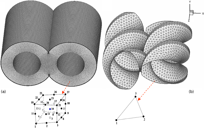
a static mesh of flow domain and b dynamic mesh (control points) for screws

Flow domain

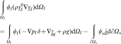
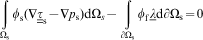
Different finite element formulations such as mixed method and penalty (continuous and discrete penalty) method have been proposed in the literature for solution of the incompressible non-Newtonian equations of continuity and motion.29, 30 In this study, the mixed method has been selected to solve the continuity and motion equations. In the mixed FEM, both velocity and pressure in the governing equations of incompressible flow are regarded as primitive variables and are discretised as unknowns. The weight residual statements of the continuity and momentum equations over element Ω_e, in a discretised domain are formulated as (11) (12) where φ_j and φ_j are appropriate weight functions, is the velocity at a previous iteration step to linearise the convection term in the discritised momentum equation.

In this study, hexahedral elements belonging to the Taylor–Hood family have been used in order to satisfy the Ladyzhenskaya–Babuska–Brezzi (LBB) condition. In these elements, the velocity and pressure fields are approximated using biquadratic and bilinear shape functions respectively. Therefore, there are 27 nodal velocity components (corner and midside of element) and eight nodal pressure component (corner of element) respectively. These elements provide unequal order interpolations for velocities and pressure. Therefore, the discritised velocity and pressure shown in equations (13) and (14) are expressed as (13) (14) Following weight residual finite element scheme, and using Galerkin method in which the weight and the interpolation functions are identical, the working flow equations of mixed scheme is derived in a matrix form as (15) where [A] and [B] are the submatrices of stiffness matrix, is the velocity vector, p is pressure and is the right hand side vector.30^–32

Coupling

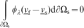
The fluid structure problems presented throughout this paper consists of a fluid domain Ω_f and a solid Ω_s domain. These two domains are coupled at the boundary of the solid domain ∂Ω_s by the constraint as (16) This constraint is applied weakly by introducing a distributed Lagrange multiplier λ.

Figure 2 represents a 2D view of fluid domain ∂Ω_f, which is discretised into hexahedral elements, with the screw boundary ∂Ω_s crossing the elements. The Lagrange multiplier is defined along the boundary ∂Ω_s to couple the velocity of this boundary to the velocity of the fluid elements in which the boundary is situated.

Figure 2

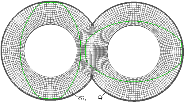
Two-dimensional view of flow domain and solid boundary immersed in fluid domain

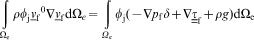
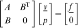
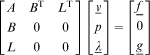
The weak form equations (2) and (8) and the constraint are described as (17) (18) (19) where φ_f, φ_s and φ_λ are appropriate weight functions. The working flow equations after coupling is derived in the matrix form as (20) where [A], [B], … are the submatrices of stiffness matrix, is the velocity vector, p is pressure, is the Lagrangian multiplier, is the right hand side vector and g is the screw velocity. 27 , 28

Solution strategy

The numerical strategy for this modelling is based on the combination of fictitious domain method and FEM that include four steps:

generation of a static mesh for the flow domain (delimited domain by barrel without the screws) (Fig. 1a)

ii.

generation of a dynamic mesh (N control point) on screw surfaces for each moving screw (Fig. 1b)

iii.

imposition of screw velocity on control points

iv.

solving continuity and motion equations using mixed FEM.

The working equations are cast into local natural coordinate system using isoparametric mapping. The members of the submatrix and subvector are then computed for each element by appropriate Gauss quadrature method. The resulting algebraic equations are assembled into a global matrix and after imposing the appropriate set of boundary conditions are solved. The presence of the convective terms in the momentum equations and also dependency of the viscosity on velocity gradient make the final set of assembled equations non-linear. Therefore, in the present work, the Picard's iterative procedure is used to handle the non-linear nature of the derived equations. 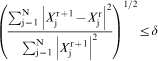The convergence criterion used in the present work is given by (21) where denotes the field velocity components corresponding to the degree of freedom j at iteration cycle r and δ is the convergence to tolerance (e.g. 10⁻³)

Particle trajectories

Using the velocity field v(x, t) the particle path in the TSE can be given by the numerical solution of equation (22) (22) This equation is solved numerically using the Euler predictor correction algorithm.13, 33 Initial position of particles is X₀ and the new position is calculated by integration of equation (22). For every time step, the solution corresponding to the new position of the screws is used to determine the new location of X. The RTD was obtained based on the calculation of particle tracers.

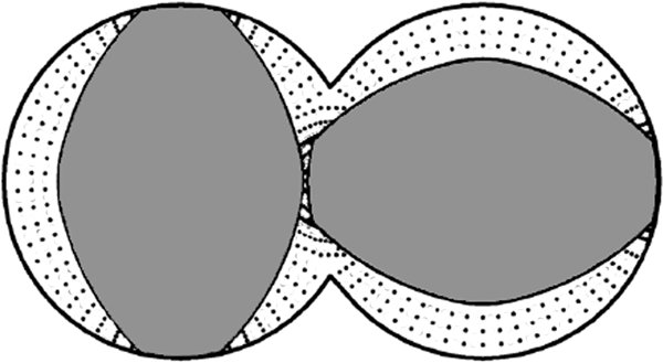
Geometry description

The geometry of conveying elements of TSEs can be defined using Booy's kinematics principles.34 The angle of intermeshing α_i is related to the tip angle which is given as (23) where α_t is the tip angle. The channel depth H(θ) as a function of angle θ can be written as34 (24) where L_c, D and δ are clearance distance of screws, screw diameter and clearance between screws and barrel respectively. A cross-section of an intermeshing TSE can be seen in Fig. 3.

Figure 3

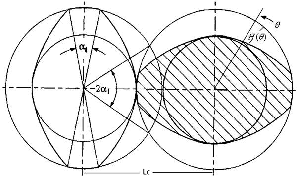
Cross-section of TSE

Boundary conditions

In this simulation no-slip boundary condition was assumed for both screw and barrel surfaces. The velocities of screws in conjunction with a fixed barrel were selected as the wall boundary conditions. Also the periodic boundary condition was applied for the inlet and outlet boundaries.

Results and discussion

Based on the combination of fictitious domain method and the mixed FEM, a computer code was developed in FORTRAN and compiled by an Intel Fortran compiler version 10.1. This code was employed to simulate the flow of a HDPE melt through the conveying region of a laboratory intermeshing corotating TSE (Brabender) as shown in Fig. 4. The polymer was supplied by Tabriz Petrochemical Co. (Tabriz, Iran), with the trade name of HDPE-5218. The rheological and physical properties of this HDPE are given in Table 1. The geometry of the flow domain was first defined by the above mentioned relations (equations (23) and (24)) and then drawn in a CAD software (SolidWorks). The geometrical specifications of conveying elements region in this extruder are recorded in Table 2. The geometry was then discretised into a finite element mesh with 32 000 hexahedral elements and 278 000 nodes belonging to the Taylor–Hood family, Q₂/Q₁ (Ref. 29) to approximate the velocity and the pressure (Fig. 1a). Also a mesh with 4500 triangles elements and 3200 nodes (control points) were used for surface of each screw (Fig. 1b). Pre- and post-processing steps in the present work were performed using two interactive commercial packages called Gambit and Tecplot respectively.

Figure 4

View of screw configuration in TSE

Table 1

Physical and rheological behaviour of HDPE melt

Material	Power law index n	η_o/Pa sⁿ	λ/s	Melt density/kg m⁻³
HDPE-5218	0·85	1130	0·95	760

Table 2

Geometrical specification of conveying region in TSE

Characteristics	Number of tips	Screw diameter D/mm	Centerline distance L_c/mm	Helix angle ψ/°	Intermeshing angle α_t/°	Clearance δ/mm
Value	2	20	17·3	45	19	0·3

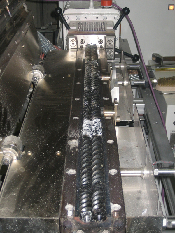
The simulations were carried out in two stages. At the first step, the flow of the polymer melt at a low screw speed (5 rev min⁻¹) was considered in order to verify the accuracy of the model by the comparison of the computed results with experimental data. This is because we have experimentally found that the conveying elements, close to the kneading discs are fully filled at low screw speeds and therefore the pressure can be accurately measured in this region. Figure 5 shows the extruder machine with inserted transducers that were used to measure the pressure at different locations. The comparison of calculated results and experimental data is shown in Fig. 6. As it can be seen, there is a good agreement between the experimentally measured data and calculated results with a relative error of less than 10%. The discrepancies can be attributed to the approximating nature of the numerical technique and also the error in the experimental measurements of the pressure.

Figure 5

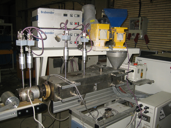
Instruments set-up used for pressure measurement

Figure 6

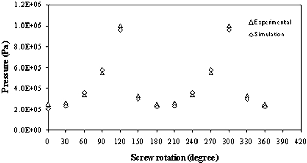
Variation of pressure against position of screws at screw speed of 5 rev min⁻¹

Having confirmed the accuracy and applicability of the developed model, the second step simulations were performed for three medium to relatively high screw speeds (10, 30 and 60 rev min⁻¹). The variation of calculated pressure with respect to the position of the screws for the selected rotational speeds has been displayed in Fig. 7. As it can be observed, the pressure changes with the rotation of the screws and two peaks are appeared for pressure at different positions of screws. These peaks are produced due to the compression of the polymer melt induced by the motion of the screw tips toward the apex. In addition, the pressure values have been increased with increasing the screw speeds.

Figure 7

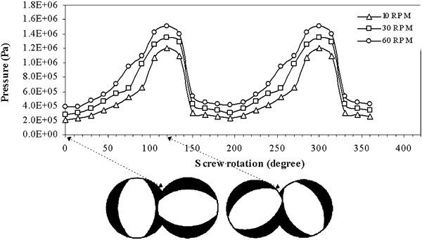
Variation of pressure against position of screws at different rotational speeds

In order to show the effect of configurations on the velocity field, a sample screw speed of 60 rev min⁻¹ was selected. Figure 8 represents the distribution of the v_x at different axial distances of conveying region. As it can be seen, the fluid undergoes a circular motion at both intermeshing and between screw and barrel regions. The flow exchanges between two screws and thus the flow movement in axial direction is reduced. This leads to increase the residence time and thus the mixing efficiency is increased at the conveying region. In addition, the variations of v_x with screw rotations for different screw speeds at apex region are shown in Fig. 9. According to this figure, the maximum transverse velocity for the exchanging of the flows occurs at θ = 135°.

Figure 8

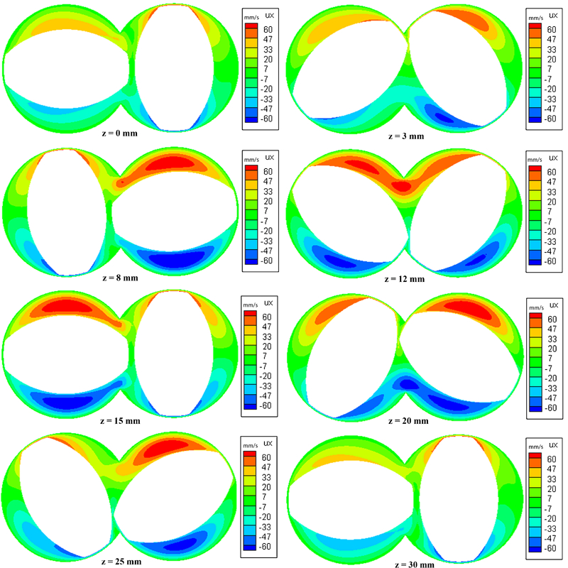
Distribution of v_x at different axial distances for screw speed of 60 rev min⁻¹

Figure 9

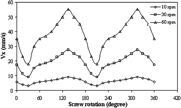
Variation of v_x at apex region with screw rotation for different rotational speeds

To understand the phenomenon of the axial movement of the fluid inside the conveying region, the v_z contours at different cross-sections have been plotted in Fig. 10. The maximum values of v_z appear in both the screw tips and intermeshing regions. These figures confirm that the positive movement (positive pumping) is the dominated mechanism for conveying in the TSE. Also, the variation of v_z with screw rotations for different screw speeds at apex region is illustrated in Fig. 11. The negative values of v_z is attributed to the reverse flow.

Figure 10

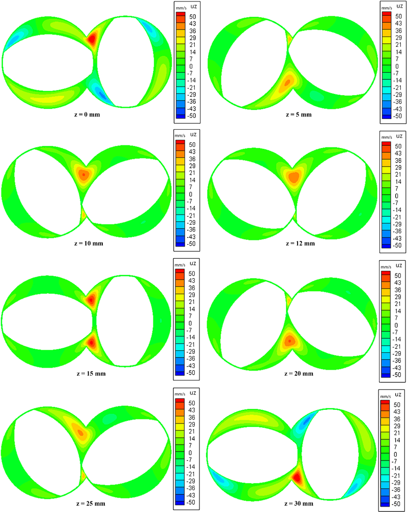
Distribution of v_z at different axial distances for screw speed of 60 rev min⁻¹

Figure 11

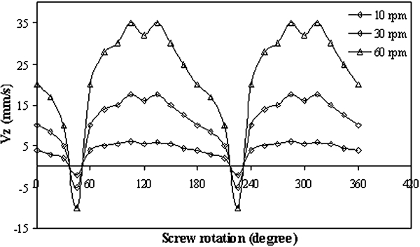
Variation of v_z at apex region with screw rotation for different rotational speeds

For the evaluation of the dispersive mixing in the TSE, the shear rate distribution has been calculated using predicted flow fields. Figure 12 shows the shear rate fields and its unevenness at different screw configurations of the conveying region. As it can be seen, the maximum values for shear rate are created in both the intermeshing region and between screws and barrel regions. Therefore, these regions have important role on dispersive mixing in the TSE. Maximum shear rate of 750 s⁻¹ has been calculated at the intermeshing region between the screw tip gap. The highest amounts of shear rate are produced in this area since the tips of screws move in opposite directions, therefore, the fluid is forced to flow through screw gap in the intermeshing region and leads to an increase in the velocity of melt in both forward and backward directions. Similar to velocity components, the variation of shear rate at apex region against rotation of screws at different screw speeds has been evaluated and shown in Fig. 13. It can be observed that the shear rate increases with decreasing the area of the apex region.

Figure 12

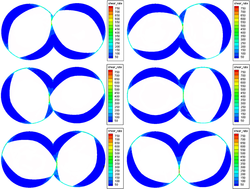
Shear rate distribution at different screw positions for screw speed of 60 rev min⁻¹

Figure 13

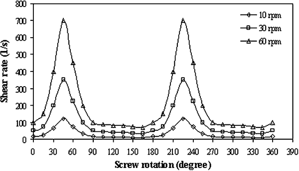
Variation of shear rate at apex region with screw rotation for different rotational speeds

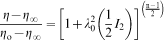
Based on experimental observations,16 the elongational flows are more effective than simple shear flows on dispersive mixing. In order to investigate and qualify the elongational and shear flow components in TSE, a previously defined parameter λ was used which is given as follows8 (25) where is the magnitude of rate of deformation tensor and |w| is the magnitude of the vorticity tensor. This parameter is used for the evaluation of the elongational and rotational flows which varies between zero and one for a pure rotation and a pure elongation respectively. It is also taken 0·5 for the case of simple shear flow. The average values of λ for different screw configurations were calculated using equation (25) and recorded in Table 3. These results are in agreement with the data reported by Manas-Zloczower et al.7, 8 The average values of λ remain almost unchanged at different screw configurations and its distribution has been shown in Fig. 14. This figure indicates that simple shear flow is the dominant flow regime in the most of the flow domain. Therefore, the efficiency of mixing improves with increasing shear rate and also residence time.

Figure 14

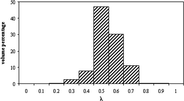
Distribution of λ for screw speed of 60 rev min⁻¹ at θ = 0°

Table 3

Average values of λ at different screw configurations

Screw configuration θ	0	30	60	90	120	150
λ	0·549	0·553	0·554	0·551	0·550	0·554

For the calculation of RTD, 420 particles were initially located at the initial cross-section of the extruder (x = 0) as shown in Fig. 15. Since the accuracy of numerical calculation of particle position will improve with decreasing the time steps, a very short time step of 0·008 s corresponding to an angle of 3° for screws rotating at the speed of 60 rev min⁻¹ was used. Furthermore, in order to avoid of the errors in the calculations of the RTD imposed by the assumption of the no-slip boundary conditions on the stationary (barrel) surfaces, the boundary layers in these regions were ignored. The results showed that the residence time of particles in the TSE depends on their initial locations. However, the particles near the barrel surface show very short axial movement because they are located near to the stationary wall. On the other hand, the particles near screw surfaces show maximum residence time because they circulate around the screws and have a rotational path in the TSE. The residence time density function F(t) is defined as the probability that the residence time is in the interval (t, t+Δt). The plot of F(t) is represented in Fig. 16. Owing to the selection of a finite number of particles in the flow domain, these curves show a scattered behaviour and therefore their analyses are very difficult. The same trends were also reported by Bravo et al.13

Figure 15

Initial locations of selected particle tracers at x = 0

Figure 16

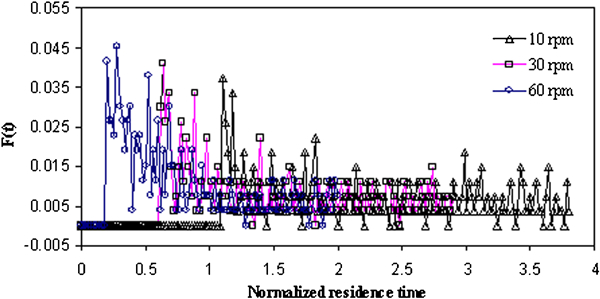
Residence time density function versus normalised residence time

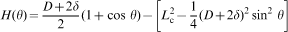
To display a smoother behaviour, cumulative distributive function H(t) was calculated using equation (26). The cumulative distributive function H(t) is defined as the probability that a particle has a residence time less than t. H(t) and is given as (26) Figure 17 displays the cumulative distribution function against normalised residence time for different screw speeds. As it is expected, the screw speed of 10 rev min⁻¹ reveals the broader distribution while the screw speed of 60 rev min⁻¹ shows the narrower distribution. Therefore, the RTD will be widened with decreasing screw speed.

Figure 17

Cumulative distribution functions against normalised residence time

Conclusions

The combination of fictitious domain method and FEM gives rise to a robust scheme for the simulation of the flow of polymeric melts in the complex geometry of the conveying region of intermeshing corotating TSEs. This technique simplifies the meshing of geometry and avoids remeshing at each time step which are normally required in traditional Lagrangian or ALE methods. The comparison of the calculated results and experimental data confirmed the ability of the present model in predicting of the flow field variables. The shear rate distribution was also employed for the evaluation of dispersive mixing efficiency in different regions of TSEs. It is shown that the maximum shear rate is appeared in both the intermeshing region and screw tips and thus regions play an important role in dispersive mixing in TSEs. The RTD can also be calculated using predicted flow fields for the evaluation of distributive mixing in TSEs. It is also found that the RTD becomes broader with decreasing screw speed.

References

Alsteens

, Legat

, Avalosse

: Int. Polym. Process. , 2004, XIX, 207–217.

Zhang

, Feng

, Chen

, Hu

: Polym. Eng. Sci. , 2009, 49, 1772–1783.

Avalosse

, Rubin

, Fondin

: J. Reinf. Plast. Compos. , 2002, 21, 419–429.

Rauwendaal

: ‘Polymer extrusion’, 4th edn; 2001, Munich, Carl Hanser Verlag.

Fukuoka

, Min

: Polym. Eng. Sci. , 1994, 34, 1033–1046.

Fukuoka

: Polym. Eng. Sci. , 2000, 40, 2524–2538.

Cheng

, Manas-Zloczower

: Polym. Eng. Sci. , 1997, 37, 1082–1090.

Cheng

, Manas-Zloczower

: Polym. Eng. Sci. , 1998, 38, 926–935.

Lawal

, Railkar

, Kalyon

: ANTEC , 1999, 45, 317–322.

10.

Mours

, Senge

, Seidl

, Wagner

, Hofmann

: Proc. Ann. Meet. PPS-17, Montreal, Que., Canada, May 2000, PPS, 21–24.

11.

Ishikawa

, Kihara

, Funatsu

: Polym. Eng. Sci. , 2001, 41, 840–849.

12.

Bravo

, Hrymak

, Wright

: Polym. Eng. Sci. , 2000, 40, 525–541.

13.

Bravo

, Hrymak

, Wright

: Polym. Eng. Sci. , 2004, 44, 779–793.

14.

Ishikawa

, Amano

, Kihara

, Funatsu

: Polym. Eng. Sci. , 2002, 42, 925–939.

15.

Zhu

, Narh

, Hyun

: Int. J. Heat Mass Tranf. , 2005, 48, 3411–3422.

16.

Elmendorp

: Polym. Eng. Sci. , 1986, 26, 418–426.

17.

Lawal

, Kalyon

, Ji

: Polym. Eng. Sci. , 1993, 33, 140–148.

18.

Ghoreishy

MHR

: Iran. Polym. J. , 1996, 5, 30–41.

19.

Ghoreishy

MHR

, Nassehi

: Adv. Polym. Technol. , 1997, 16, 45–68.

20.

Glowinski

, Pan

, Periaux

: Comput. Methods Appl. Mech. Eng. , 1994, 111, 283–303.

21.

Glowinski

, Pan

, Hesla

, Joseph

: Int. J. Multiphas. Flow , 1999, 25, 755–794.

22.

Glowinski

, Pan

, Hesla

, Joseph

, Periaux

: Int. J. Numer. Methods Fluids , 1999, 30, 1043–1066.

23.

Bertrand

, Tanguy

, Thibault

: Int. J. Numer. Methods Fluids , 1997, 25, 719–736.

24.

Bertrand

, Thibault

, Delamare

, Tanguy

: Comput. Chem. Eng. , 2003, 27, 491–500.

25.

Kruijt

PGM

, Galaktionov

, Peters

GWM

, Meijer

HEH

: Int. Polym. Process. , 2001, XVI, 161–171.

26.

Bird

, Stewart

, Lightfoot

: ‘Transport phenomena’; 2002, New York, John Wiley & Sons.

27.

Baaijens

FPT

: Int. J. Numer. Methods Fluids , 2001, 35, 743–761.

28.

van Loon

, Anderson

, de Hart

, Baaijens

FPT

: Int. J. Numer. Methods Fluids , 2004, 46, 533–544.

29.

Donea

, Huerta

: ‘Finite element methods for flow problems’; 2003, Chichester, John Wiley.

30.

Nassehi

: ‘Practical aspects of finite element modeling of polymer processing’; 2002, Chichester, John Wiley.

31.

Ghoreishy

MHR

, Razavi-Nouri

: Iran. Polym. J. , 1998, 7, 277–287.

32.

Ghoreishy

MHR

, Razavi-Nouri

, Naderi

: Comput. Mater. Sci. , 2005, 34, 389–396.

33.

Gerald

, Wheatley

: ‘Applied numerical analysis’, 7th edn; 2004, Reading, PA, Pearson/Addison-Wesley.

34.

Booy

: Polym. Eng. Sci. , 1978, 18, 973–984.