Durability models for GRC: uncertainties on strength predictions

Abstract

Even though several models exist in the literature to predict the strength durability of glass fibre (textile) reinforced concrete (GRC), a considerable gap still exists between theory and practice. No real guidelines are available for testing, model calibration and model selection. This work analyses all the uncertainties in the GRC strength durability determination process. The paper addresses the determination of the best approximating model by applying a statistical model selection method (Akaike's information criterion) on an extensive series of accelerated aging tests; a theoretical approach is presented which enables the user to check the reliability of the model selection. A method is presented for the determination of the uncertainty in the strength prediction, taking into account both the statistical distribution present on the (tensile) strength of the GRC material as well as the effect of model calibration based on a limited set of accelerated aging tests.

Keywords

Glass fibres GRC Durability Aging AIC Predictions

Introduction

Fibre reinforced concrete was initially developed to circumvent the inherent brittle behaviour of concrete. Concrete composites with high tensile strength and ductility can be obtained by reinforcing cement pastes or mortars with continuous glass fibre strands. When a glass fibre textile reinforcement (TRC) is used in a cementitious matrix, the load bearing capacity of the concrete can be enhanced in such a manner that steel reinforcement may be omitted. The TRC is of particular potential value for freeform architecture since the combination of the flexibility imparted by the high volume fraction of fibres and the lack of need for a ‘cover’ thickness of concrete to protect the steel allows thin, lightweight elements to be produced.

However, advanced glass fibre TRC composites may be subject to reduction in their mechanical properties with aging, especially in wet or moist environments.1^–8 Loss of tensile strength is a significant manifestation of this aging. Prediction of the service life of glass fibre reinforced concrete (GRC) composites in various climates is performed using an accelerated aging technique. Immersion in water for various periods of time and at various temperatures from ∼20 to ∼80°C is the most commonly used accelerating environment.1 The changes in the mechanical properties induced by such exposure are assessed, and a model is then fitted through the experimentally obtained results. However, until recently, it has not been clear whether these models provide reliable predictions of the long term performance. The effect of the scatter on the experimental results (which can be up to ±15% in some studies) on the selection, calibration and application of the models has not been studied at all. Before these models can be used with confidence for strength retention predictions in structural elements, the following aspects should be thoroughly studied for statistical robustness:

selection of the best approximating strength durability model

ii.

the sensitivity of the model selection to sufficient/insufficient experimental data

iii.

the uncertainty inherent in strength predictions due to the material and the experimental set-up uncertainties

iv.

implications of uncertainties on component design for structural applications.

This paper presents a model selection method which allows the best approximating model to be applied to the dataset at hand, weighing up the additional complexity of adding more parameters to the durability equation against the enhanced fit to the experimental data. An approach is presented which allows the user to establish whether the experimental programme used to obtain the accelerated aging dataset will allow a correct and unbiased determination of the best approximating model and thus whether the dataset can provide insights into the degradation mechanisms involved. Once this model uncertainty has been dealt with, attention is directed to prediction uncertainties. Special attention is given to the repercussions of the scatter of experimental results on the strength predictions and consequent structural detailing. A theoretical approach is presented which enables the user to predict the uncertainty in a strength prediction taking into account the acceleration scheme used, the number of specimens used for each average time–temperature point within the accelerated aging test and the statistical distribution of the failure strength of the specimens. The paper concludes with a case study of a sandwich wall panel with TRC faces, providing insight into the practical implications of prediction uncertainties on structural design.

Best approximating model

Over the years, several strength durability models have been developed for GRC, as detailed in Ref. 1. Of most interest are models based on feasible physical contexts, e.g. flaw growth based models2^–5 or bond evolution models.6^–8 In order to make strength durability predictions, one needs to determine which of the candidate models might best represent the data at hand and thus infer the degradation mechanism behind the strength loss. The user needs an effective and objective means for the selection of the ‘best approximating model’, taking into account both the fit and the ‘degree’ of the model (i.e. the number of model parameters that needs to be determined in order to fit the model to the dataset). Several model comparison methods can be found in the statistics literature. They can be divided into two main categories: methods based on null hypothesis testing and methods based on information theory. Model selection through hypothesis testing is well established. In these methods, it is generally assumed that the simpler model (the one with the fewest parameters) is correct and provides the null hypothesis. The potential improvement of the fit of another more complicated candidate model is then evaluated, leading to either the rejection or confirmation of the null hypothesis at a certain arbitrary threshold ‘P value’ (the probability that sets are identical). Methods based on a combination of information theory and statistics are a relatively new approach. The application of non-linear regression has increased progressively over the last decade in many fields.9 Akaike's information criterion (AIC),10 which combines maximum likelihood theory, information theory and the concept of the entropy of information, is one of the many methods that fall within this category. The AIC is not a validation test for a model in the sense of hypothesis testing, but it is a test between several models. This method not only allows the user to calculate which model is most likely to be correct (i.e. is the best approximating model) but also quantifies how much more likely the model is to be the best fit compared with the other candidate models. The theoretical background of the method is beyond the scope of this present paper, and for further information, the reader is encouraged to read Refs. 11 and 12, which provide a deeper insight. The AIC method was chosen for this work because of its ease of use and its good predictive properties (even though it sometimes selects a more complex, higher degree model). Alternative advanced methods, such as the minimum description length, 13 , 14 are more suitable for physical interpretation (measurement of physical process parameters) but are not efficient for prediction purposes.

Approach

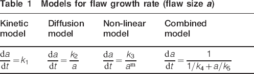
When confronted with the analysis of accelerated aging tests, one first needs to gather suitable candidate models from the literature based on a sound physical background. In this paper, four flaw growth models are taken into consideration:

the linear or kinetic model

ii.

the square root or diffusion model

iii.

the non-linear model

iv.

the combined model.

These models were presented and discussed in detail in Ref. 1, and their formulae are given in Table 1. The simplest model is the linear or kinetic model, which considers the reduction in tensile strength (at constant temperature) to be attributed to a constant fibre flaw growth rate with time (i.e. it invokes a ‘kinetic’ physical background). The square root or diffusion model supposes a gradually decreasing flaw growth rate with time (‘diffusion’ physical background). The non-linear model adds a power law dependence to this flaw growth rate modelling, while the combined model concatenates the linear and square root models (assuming initially ‘kinetic’ driven flaw growth, gradually moving to ‘diffusion’ controlled flaw growth). The temperature dependence of the rate coefficients k_i is assumed to follow an Arrhenius type relationship, with E_A,i as the activation energy of the chemical reaction (1) All the parameters relative to each of the candidate models need to be determined by fitting models to the available data, which can be performed in various ways. One can for instance determine all the rate coefficients at each separate temperature independently and then construct the Arrhenius relationship. This fitting procedure is generally adopted in the GRC literature (e.g. Refs. 2–5) and was also applied in Ref. 1. One can, however, also fit the Arrhenius relationship on the whole dataset (over all temperatures simultaneously) and thus determine the activation energy E_A,i and reference rate coefficient k_0,i for each occurring chemical reaction. This method was used in this paper, since for model comparison purposes, the estimated parameters need to be determined on exactly the same data. Looking at the individual candidate models, this fitting procedure implies that for the kinetic and diffusion models, two parameters need to be determined (namely, the respective activation energies E_A,1 and E_A,2 and the reference rate coefficients k_0,1 and k_0,2), while for the combined model, four parameters need to be estimated (two for the kinetic part and two for the diffusion part of the reaction). For the non-linear model, three parameters need to be fitted: the activation energy E_A,3, the reference rate coefficient k_0,3 and the m parameter.1

Table 1

Models for flaw growth rate (flaw size a)

Kinetic model	Diffusion model	Non-linear model	Combined model

In general, the previous GRC studies have based the selection of the ‘best fit’ strength durability model solely on the sum of squares values,2^–5 i.e. by minimising the total absolute error between the model curve and the experimental data. The model obtained in this manner is referred to as ‘the best fitting model’. One should, however, take into consideration two additional aspects when comparing candidate models: the number of parameters that need to be estimated and the amount of data to which the models are fitted. First, the improvement in sum of squares needs to be sufficiently large to justify adding extra parameters to the strength durability equation. Second, the dataset also needs to be sufficiently large to justify adding extra parameters. 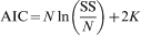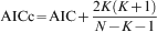These factors can be taken into account by implementing AIC, which was developed in the mid 1970s.9^–12 If it assumed that the errors are normally distributed with a constant variance for all the models in the set, then the AIC can be written in the following form (2) where N is the number of data points, SS is the sum of squares of the vertical distances between the data and the model and K is the number of parameters +1 (since the SS is also estimated).

To take into account smaller datasets15^–18 with a relatively high value for K compared to N, a modification of the criteria can be found in the literature [corrected AIC (AICc)] (equation (3)). This modified AIC (AICc) can be used for all datasets (be it large or small datasets) since the AICc value will approximate the AIC value when a large dataset is being analysed (equation (3)) (3) The model corresponding to the smallest AICc (or AIC) value is more likely to be the ‘best approximating model’ of the candidate models; however, the procedure does not quantify how much more likely. To quantify the relative likelihood of a model being the best approximating model, one needs to determine Akaike's weights ω_i (4) with (5) ω_i provides the weight of evidence in favour of model, with i being the best approximating model for the particular dataset under study, given that one of the R candidate models is the best approximating model. Further on in this paper, the model obtained after comparing the respective Akaike's weights will be referred to as ‘the best approximating model’.

Results and discussion

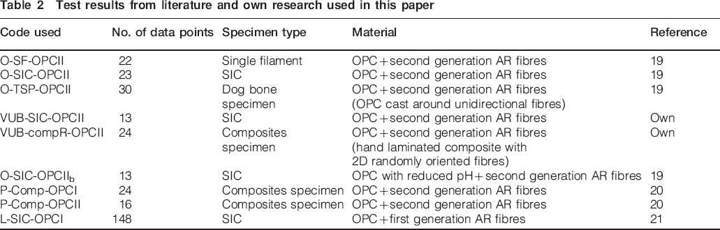
To illustrate the method elaborated above, datasets obtained from a wide variety of test methods and material combinations, taken both from the literature as well as generated specifically for this paper, were modelled accordingly. Details of the datasets can be found in Table 2. The two datasets with the prefix VUB (i.e. VUB-SIC-OPCII and VUB-compR-OPCII) were produced specifically for this paper. They are made with the microconcrete developed in Ref. 19, which was also used for the datasets (O-SIC-OPCII and O-TSP-OPCII) and forms the basis for the pore solution used as an aging medium for the dataset O-SF-OPCII. The modified strands in cement specimens developed in Ref. 22 are used for the dataset VUB-SIC-OPCII. The other dataset (VUB-compR-OPCII) is full of composite laminate (TRC) specimens produced by a hand lay up technique [with a two-dimensional (2D) random fibre volume fraction of ≈9% and a specimen thickness of 3–4 mm], analysed by means of tensile testing after exposure to an accelerated aging environment.

Table 2

Test results from literature and own research used in this paper

Code used	No. of data points	Specimen type	Material	Reference
O-SF-OPCII	22	Single filament	OPC+second generation AR fibres	19
O-SIC-OPCII	23	SIC	OPC+second generation AR fibres	19
O-TSP-OPCII	30	Dog bone specimen	OPC+second generation AR fibres (OPC cast around unidirectional fibres)	19
VUB-SIC-OPCII	13	SIC	OPC+second generation AR fibres	Own
VUB-compR-OPCII	24	Composites specimen	OPC+second generation AR fibres (hand laminated composite with 2D randomly oriented fibres)	Own
O-SIC-OPCII_b	13	SIC	OPC with reduced pH+second generation AR fibres	19
P-Comp-OPCI	24	Composites specimen	OPC+second generation AR fibres	20
P-Comp-OPCII	16	Composites specimen	OPC+second generation AR fibres	20
L-SIC-OPCI	148	SIC	OPC+first generation AR fibres	21

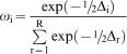
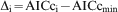
The best approximating (according to the AIC method) and best fitting (according to simple minimisation of sum of squares error) strength durability models for each of the individual results in Table 2 were determined using the following approach. First, candidate models with a sound physical basis were selected. As mentioned in the section on ‘Approach’, four feasible flaw growth models were considered in this work. These models were expressed in terms of the rate of change of flaw size, known as the ‘size rate’ approach (for more details, see Ref. 1). Second, for each dataset and each model, the corresponding model parameters were determined by optimising the fit with the experimental results. Third, with the help of the AIC, the best approximating model was determined (equations (3) and (4)) by taking into consideration the sum of squares (SS) value, the number of data points and the number of model parameters within each strength durability model. Table 3 gives the SS and related AIC corresponding to the best fit of the individual strength durability models (K denotes kinetic model, D denotes diffusion model, N denotes non-linear model and C denotes combined model). The AIC values give the weight of evidence ω_i in favour of the model being the best approximating model of the models under consideration (e.g. if D = 70%, there is a 70% chance that the diffusion model is the best approximating model of those considered for the data at hand). The bold areas within Table 3 indicate both the best fitting model (with the lowest sum of squares) as well as the best approximating model (with the highest weight of evidence ω_i) for the dataset under study.

Table 3

Listing of sum of squares and AIC values for all models under study and for each result from literature and own research (Table 2)*

	Sum of squares				AIC using SS ω_i/%
	K	D	N	C	K	D	N	C
O-SF-OPCII	0·1961	0·0531	0·0381	0·0527	0	6·2	93·5	0·3
O-SIC-OPCII	0·1311	0·0365	0·0247	0·0365	0	4·7	95·1	0·2
O-TSP-OPCII	0·1446	0·0877	0·0845	0·0877	0	65·8	30·1	4·1
VUB-SIC-OPCII	0·0709	0·0358	0·0232	0·0340	0·4	34·0	65·3	0·3
VUB-comp-OPCII-R	0·1446	0·0855	0·0790	0·0852	0·1	60·4	36·5	2·9
O-SIC-OPCII_b	0·068	0·0846	0·0665	0·0462	68·4	16·5	9·1	6·0
P-Comp-OPCI	0·0333	0·0350	0·0220	0·0164	0·4	0·2	12·8	86·6
P-Comp-OPCII	0·0855	0·0985	0·0818	0·0800	63·1	20·3	14·6	2·0
L-SIC-OPCII	0·7230	0·3438	0·3021	0·2680	0·0	0·0	0·0	100

*K denotes kinetic model, D denotes diffusion model, N denotes non-linear model and C denotes combined model.

If model selection were solely to be performed on the basis of the SS values, the higher degree models (N and C) seem to better fit all the datasets at hand; this is expected since adding more parameters to the model will decrease the SS. Checking whether the reduction in SS justifies the introduction of more parameters using the AIC, the relevance of the lower degree models improves (four of the nine datasets under study). However, in five of the nine datasets, the best fitting model (N or C) remains the best approximating model. The degradation mechanism and thus also the best approximating model are likely to depend on the material combination used (the matrix formulation, the type of AR glass fibres, type of coatings on the fibres, etc.) and the specimen type. As a result, one certainly can not, in a general sense, state that a specific model will be the best approximating model for all standard GRC applications.

Four specific results within Table 3, i.e. O-SF-OPCII, O-SIC-OPCII, P-Comp-OPCI and L-SIC-OPCII, are of particular interest. All of these results show a relatively high weight of evidence in favour of a higher degree model (C or N). The results denoted as L-SIC-OPCII are the most detailed dataset available in the literature (see Table 2), and the evidence in favour of the combined model is significant (100%), indicating that this model seems to accurately describe the occurring degradation (this was also visually confirmed by checking the experimental residual strength versus exposure time plots with the proposed best approximating model). The other three results are more limited (23 to 25 data points); nonetheless, the evidence in favour of the higher degree models is also substantial (>85%).

Table 4 shows the model parameters corresponding to the best SS fit of the studied datasets for each candidate model. The contribution of the kinetic part of the combined model becomes negligible when the m parameter reaches a value <0·59 (indicated in bold) (i.e. the activation energy E₄ of the kinetic reaction reaches a value of zero, and the reference rate of the kinetic reaction becomes either infinite or very small [parameters in bold]).

Table 4

Model parameters corresponding with best SS fit for each dataset under study (Table 2) and for each candidate model*

	K		D		N			C
	E₁/kJ mol⁻¹	ln k_0,1/per day	E₂/kJ mol⁻¹	ln k_0,2/per day	E₃/kJ mol⁻¹	ln k_0,3/per day	m	E₄/kJ mol⁻¹	ln k_0,4/per day	E₅/kJ mol⁻¹	ln k_0,5/per day
O-SF-OPCII	91	32	116	43	128	48	0·38	0	→∞	…	…
O-SIC-OPCII	76	25	94	33	108	39	0·36	0	→∞	…	…
O-TSP-OPCII	84	28	97	35	102	37	0·42	0	→∞	…	…
VUB-SIC-OPCII	75	25	91	32	133	49	0·24	0	N/A	103	43
VUB-comp-OPCII-R	43	13	47	15	49	17	0·38	0	N/A	49	23
O-SIC-OPCII_b	63	19	69	22	61	18	1·43	52	19	42	54
P-Comp-OPCI	100	35	108	39	103	36	0·7	82	32	159	66
P-Comp-OPCII	76	25	83	29	78	26	0·79	80	30	68	32
L-SIC-OPCII	89	31	93	34	92	33	0·59	92	37	91	41

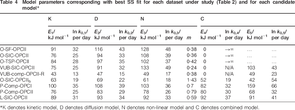
*K denotes kinetic model, D denotes diffusion model, N denotes non-linear model and C denotes combined model.

Coefficients of variation (CVs) of 10–15% on the experimental results are quite common for GRC, and often, only a very small number of replicates (three to four) are used. This scatter might have a considerable influence on the accelerated aging tests and the determination of the best approximating model. To address this problem, cost functions V can be used instead of the sum of squares method. This approach takes into consideration the scatter of the individual test results and the number of replicates, which lead to each individual average data point. 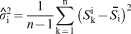As a result, the datasets are more robustly fitted: data points with a relatively high scatter are filtered out while a focus is put on results with a limited scatter (6) with (7) where n is the number of experimental results S_k which give rise to the average data point , ϵ represents the difference between and the model prediction, while N is the number of data points. It should be mentioned that equation (6) can be statistically justified for test series that are the result of six or more tested samples.23

This approach is combined with the AIC approach in Table 5. The cost procedure could only be executed on six of the nine results from Table 3 since, for the other datasets, the values of the individual results were not available. In four out of the six datasets, only minor differences are recorded in comparison to Table 3: the obtained best fit models (in bold) remain the same as the ones obtained with the SS method in Table 3. For these four datasets, the best approximating models (in bold) also remain invariant, although the weight of evidence in favour of these best approximating models differs. One should, however, remain vigilant, since the higher scatter on the results from the two other datasets in Table 5 (O-SIC-OPCII and VUB-comp-OPCII-R) would lead to an inaccurate determination of the best approximating model if this scatter were to be neglected. For example, considering the result (VUB-comp-OPCII-R), the weight of evidence in favour of the diffusion model drops from 60·4% with the SS method to 3·7% for cost functions, and the non-linear model increases from 36·5 to 96·1%. A similar behaviour can be seen for the result (O-SIC-OPCII) where the evidence in favour of the diffusion model becomes very convincing when using the cost functions, while when using the SS method, the weight of evidence in favour of the non-linear model was more convincing. A high scatter on even a few results within the whole dataset, or some data points that are the result of a smaller number of replicates, might lead to an inaccurate determination of the underlying mechanisms and, as a result, incorrect selection of the strength durability model. The results within Table 5 indicate that such factors must be considered, e.g. using cost functions, for the analyses of GRC accelerated aging tests. Results obtained using specialised aging specimens (e.g. SIC or simulated pore solutions) must be treated with extreme care if used to predict the strength of composite specimens, even if the material combination is exactly the same. When looking at the first five results within Table 5 (O-SF-OPCII, O-SIC-OPCII, O-TSP-OPCII, VUB-SIC-OPCII and VUB-comp-OPCII-R), all of which were made using the same material combination (or simulated in case of O-SF-OPCII, based on the same material combination), the modelling suggests that the same degradation mechanism may not be operating in all cases (in two cases, the diffusion model was returned, and in three cases the non-linear model). Table 6 gives the model parameters corresponding to the best fit models presented in Table 5. From these values (in bold), similar conclusions can be drawn as from Table 4.

Table 5

Listing of cost function and AIC values for all models under study and for each result from literature and own research (Table 2)*

da/dt	Cost function				AIC using CF ω_i/%
da/dt	K	D	N	C	K	D	N	C
O-SF-OPCII	282·29	70·25	31·07	67·91	0	0	100	0
O-SIC-OPCII	315·02	101·92	84·15	101·93	0	70·0	17·1	12·8
O-TSP-OPCII	133·59	70·47	66·49	69·37	0	58·6	36·8	4·6
VUB-SIC-OPCII	50·56	29·25	19·06	27·27	1·0	34·5	64·1	0·4
VUB-comp-OPCII-R	215·26	108·24	73·17	108·24	0	3·7	96·1	0·2
O-SIC-OPCII_b	103·45	108·77	103·40	92·24	54·0	39·0	6·2	0·8

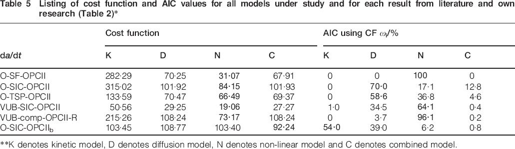
**K denotes kinetic model, D denotes diffusion model, N denotes non-linear model and C denotes combined model.

Table 6

Model parameters corresponding to best cost function fit for each dataset under study (Table 5) and for each candidate model*

	K		D		N			C
	E₁/kJ mol⁻¹	ln k_0,1/per day	E₂/kJ mol⁻¹	ln k_0,2/per day	E₁/kJ mol⁻¹	ln k_0,1/per day	E₂/kJ mol⁻¹	ln k_0,2/per day	E₁/kJ mol⁻¹	ln k_0,1/per day	E₂/kJ mol⁻¹
O-SF-OPCII	81	28	114	42	146	55	0·34	0	→ ∞	…	…
O-SIC-OPCII	82	27	101	36	112	41	0·40	0	→ ∞	…	…
O-TSP-OPCII	85	29	93	33	97	35	0·41	0	→ ∞	…	…
VUB-SIC-OPCII	74	24	92	32	140	53	0·22	0	N/A	105	44
VUB-comp-OPCII-R	39	11	44	14	57	21	0·26	0	→ ∞	…	…
O-SIC-OPCII_b	54	16	63	19	54	16	0·94	122	47	40	18

*K denotes kinetic model, D denotes diffusion model, N denotes non-linear model and C denotes combined model.

Reliability of model selection

When analysing an experimentally obtained dataset, one should always check the reliability of the model selection for a given dataset. If the dataset is not robust, e.g. not enough data points, not enough temperatures, few replicates or significant scatter on the test results, then the best approximating model obtained using the approach given in the section on ‘Best approximating model’ of this paper might be misleading. A procedure is presented here to establish whether the dataset is robust enough to be used to ascertain the mechanisms behind the degradation (i.e. determine which is the best approximating model) and/or to be adopted for strength prediction purposes. This procedure will be used (see the section ‘Results and discussion’) to evaluate the datasets, within Table 5, for which the best approximating models were determined using the cost function method.

Approach

The various steps in the procedure are schematically depicted in Fig. 1. During the initial step (step 0), it is assumed that the best approximating model obtained using the cost function method given in the section on ‘Results and discussion’ correctly represents the mechanisms behind the degradation of the material at hand (for instance for the dataset VUB-comp-OPCII-R, the best approximating model corresponds to the non-linear model with the model parameters given in Table 6). The model parameters thus obtained are used to construct a hypothetical residual strength versus time dataset (for the dataset VUB-comp-OPCII-R, this thus implies that curves are constructed at 30, 50 and 80°C, these being the temperatures at which the real experiments were carried out). The construction of these curves allows the determination of the hypothetical residual strengths for each time–temperature point related to the experimental programme which was carried out (for the dataset VUB-comp-OPCII-R for instance, tests were carried out at 30°C after 10, 15, 21, 30, 35, 37·5, 75, 90 and 120 days, at 50°C after 5, 11, 15, 21, 35, 75 and 112 days and at 80°C after 2, 5, 8, 10, 11, 15, 21 and 30 days). In the following step (step 1), random generated scatter, intended to simulate that expected to be present on real experimental results, is applied to these hypothetical data points. As a first approximation, the scatter present on all the results is assumed to be equal to the scatter present on the unaged control specimens. A two-parameter Weibull distribution is assumed (such a distribution is generally recognised for the strength of glass fibres24). In step 2, the procedure presented in the section on ‘Results and discussion’ is applied to these artificially scattered data points. For each of the individual models (K, D, N and C), the best fit model parameters and associated cost functions are determined. In step 3, Akaike's weights are determined using the cost functions, allowing the determination of the best approximating model for the simulated dataset. Steps 0 to 3 are repeated 100 times, determining the best approximating model each time.

Figure 1

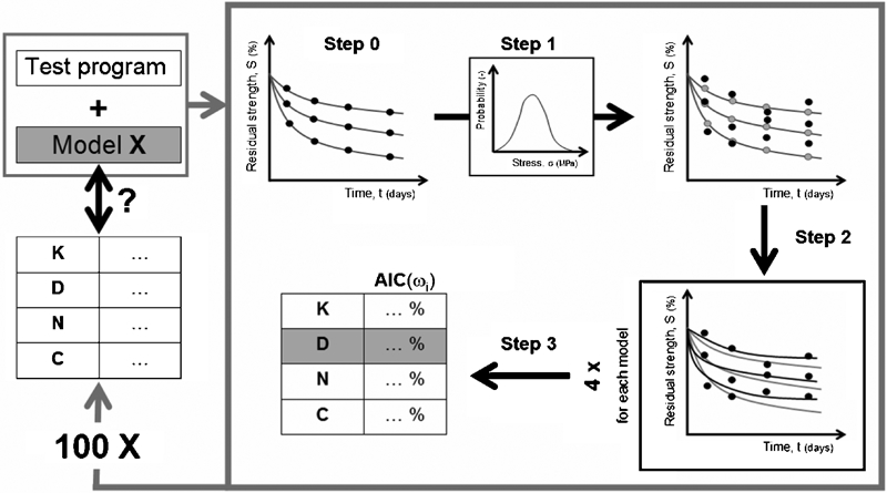
Scheme of theoretical method used for determination of reliability of calibration

Results and discussion

The procedure elaborated in the section on ‘Approach’ is applied to the results in Table 5, and the results are presented in Table 7. The table shows the number of instances (out of the 100 simulations) in which each of the four candidate models were selected as the best approximating model for the dataset under study &lpar (maxima in bold);maxima in bold). For each of the datasets, a summary of the essential aspects of the experimental set-up is also provided (average number of specimens used, number of experimental temperatures, number of time–temperature data points and CV on the reference specimens). These results clearly indicate that for four of the six datasets (O-SF-OPCII, O-SIC-OPCII, O-TSP-OPCII and O-SIC-OPCIIb), the scatter on the experimental dataset might influence and/or obscure the determination of the best approximating strength durability model. One should thus remain vigilant when handling these results. For the other two datasets however (VUB-SIC-OPCII and VUB-comp-OPCII-R), the model selection is very reliable since the expected model is retrieved in >95% of the simulations. For one of the six datasets under study (O-TSP-OPCII), the scatter on the accelerated aging data makes it particularly difficult to correctly determine the best approximating model; only in 58 of the 100 simulations is the ‘correct’ (initial) best approximating model retrieved. The reason for this behaviour is not immediately clear from the details of the experimental set-ups. A reasonable number of time–temperature points (30 in total) and temperatures (four) are used compared to the other datasets under study. In addition, the scatter on the reference specimens is quite low, with a CV of only 7·2%. However, the average number of replicates used is relatively low (3·2 specimens). Nevertheless, within concrete testing, studies using such a limited amount of specimens are not uncommon. These results suggest that using a small number of replicates cannot be compensated for by using more time intervals or aging temperatures or justified by invoking a low CV. For illustrative purposes, an alternative experimental dataset is constructed based on the dataset O-TSP-OPCII. All the time–temperature points which were the result of less than four replicates (in the original experiment) are assumed to result from experiments on four replicates; all the time–temperature points resulting from less than five replicates are assumed to be the outcome of five replicates. When using at least four or five specimens in the dataset, the diffusion model is respectively picked in 66 and 81 of the 100 simulations. The importance of the number of specimens for the selection of the best approximating model thus becomes very clear. The dataset O-TSP-OPCII is discounted from this point on, owing to the apparent unreliability of test procedure used to generate the results.

Table 7

Reliability of the dataset for the selection of the best approximating model*

	K	D	N	C	Average number of specimens	Number of temperature	Number of data points	CV ref./%
O-SF-OPCII	0	11	88	1	8·5	3	22	14·9
O-SIC-OPCII	1	73	20	6	6·5	3	23	10·3
O-TSP-OPCII	5	58	28	9	3·2	4	30	7·2
VUB-SIC-OPCII	0	2	98	0	10	3	13	9·6
VUB-comp-OPCII-R	0	1	99	0	5	3	24	9·1
O-SIC-OPCII_b	86	11	3	0	7·8	3	13	6·9

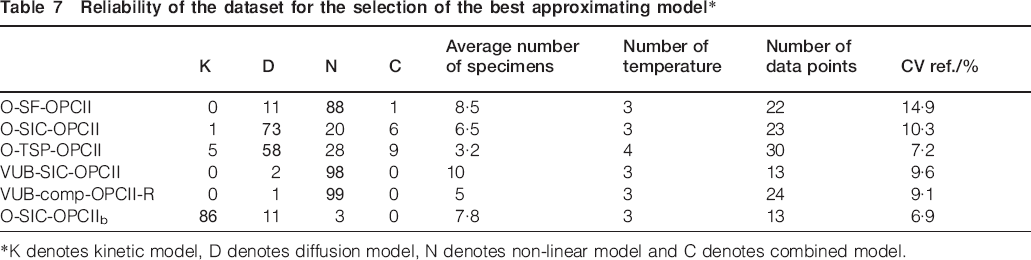
*K denotes kinetic model, D denotes diffusion model, N denotes non-linear model and C denotes combined model.

Uncertainty in strength predictions

Once the best approximating model has been determined and checked (see the sections on ‘Best approximating model’ and ‘Reliability of the model selection’), one should establish the magnitude of the uncertainty in a strength prediction, taking into account the variation in the dataset. Ignoring the effect of this uncertainty might lead to structural elements, which are not properly dimensioned and thus potentially unsafe. An approach is presented below which will enable the user to determine the uncertainty in strength predictions, taking into account the scatter on the experimental results, the number of experiments performed and the specific accelerated aging test scheme used.

Approach

The method presented in this section consists of four steps, which are illustrated in Fig. 2. This scheme presents some similarities with Fig. 1 (see the section on ‘Approach’). First, theoretical curves are once again constructed (step 0 in Fig. 2) for all the temperatures within the studied accelerated aging test scheme using the best approximating model obtained in the section on ‘Results and discussion’. In step 1, the time–temperature points of these theoretical curves, corresponding to tests performed within the experimental programme, are adjusted to simulate scatter on the results. For the distribution function, the scatter present on the control specimens is taken as a reference (see the section on ‘Approach’). Once all the data points have been adjusted, taking into account the scatter present on the results in step 2, the model parameters for each candidate model are determined with the same method as discussed in the section on ‘Best approximating model’. Then, the best approximating model is determined. If the best approximating model corresponds with the initial best approximating model, then the parameters are retained (in all the other cases, the results are discarded). With these model parameters, the residual strength after 10 years of Belgian outdoor weathering is determined, e.g. as a first approximation, an average temperature of 11°C and a constant relative humidity of 100% were used over X years of Belgian outdoor weathering. The procedure shown in Fig. 2 is then repeated 10000 times. Comparison of the obtained residual strengths after X years of outdoor exposure S_VXyears with the initial theoretical residual strength S_TXyears gives an order of magnitude for the uncertainty on the prediction. To determine the uncertainty margin with the 10000 simulated values for S_VXyears, the distribution is plotted in a graph similar to the one presented in Fig. 2. On this density distribution, the 95% confidence interval is then determined [illustrated by the lower limit (LL) and upper limit (UL) in Fig. 2]. Since for strength predictions, working with higher values than S_TXyears might result in underdimensioned elements, the expression presented in equation (8) for the uncertainty margin was chosen (8) One should, however, also take into consideration the uncertainty on the material properties during the design of GRC structural elements. The assumption is made that the scatter present on the control specimens is representative for the distribution of the strength (Fig. 3a). On this density distribution, once again, the 95% confidence interval can be determined [illustrated by the LL material (LLM) and UL material (ULM) in Fig. 3a]. Since for strength predictions, lower material properties might also result in underdimensioned elements, the expression presented in equation (9) was chosen for the uncertainty margin (9) In Fig. 3, the total uncertainty is thus defined as the combination of both uncertainties (uncertainty_test and uncertainty_mat).

Figure 2

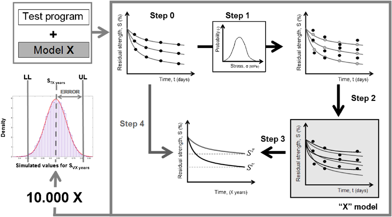
Scheme of theoretical method used for determination of uncertainty on strength prediction

Figure 3

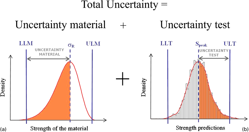
a density distribution of strength of material (Weibull distribution was assumed in this figure since this is for strength of glass fibres) and b density distribution of strength prediction (resulting from utilised test set-up)

Results and discussion

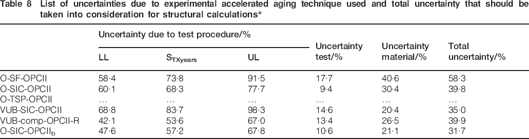
Table 8 shows the uncertainty due to the distribution on the strength of the material for all the datasets in Table 7 except O-TSP-OPCII. This information is determined, as described previously, from non-aged control specimens. For all the series under consideration, this reference was composed out of a minimum of 10 and a maximum of 20 specimens. From the results presented in Table 8, it is clear that the scatter on GRC specimens is relatively high, independent of the type of specimen used, and generally lies between 20 and 30%. The only exceptions are the single filament specimens (O-SF-OPCII), where the material uncertainty of up to 40% was recorded. This very high scatter is directly related to the delicate specimen preparation technique and the fact that the individual filament strength is measured rather than an average, as is the case for composite specimens and SIC specimens. Table 8 also gives the list of uncertainties attributed to the experimental accelerated aging technique used. These values are obtained after application of the theoretical method presented in the section on ‘Approach’ and depicted in Fig. 2. Compared to the material uncertainty, the uncertainty owing to the test procedure is low, ranging between approximately 10 and 20%. The highest value is again recorded for the O-SF-OPCII series, which is once more directly related to the high scatter present on the specimens. When observing the last column of Table 8, which gives the total uncertainty that should be taken into account when confronted with strength predictions (ignoring the O-SF-OPCII results for the reasons given above), a general uncertainty of between 30 and 40% should be taken into account in structural applications; this is not negligible. For example, if a given strength durability model suggests a ‘mean’ or deterministic residual strength of 70% after a given elapsed time, another 40% would have to be subtracted (for a similar material as that used in the VUB-comp-OPCII-R tests), resulting in a ‘characteristic’ or safe residual strength of only 30%. This uncertainty margin will have a major influence on structural design applications. Further analysis of Table 8 suggests that the three datasets that initially use the non-linear model as the best approximating model give rise to higher uncertainty margins attributable to the uncertainties in the test procedure. Whether this behaviour is a direct result of the use of a higher degree durability model is not completely clear. However, if the datasets VUB-SIC-OPCII and O-SIC-OPCIIb are compared, which are both the results of testing relatively large numbers of specimens (10 and ∼8 specimens for each data point) with a relative low scatter (CV ≈9 and ≈7%) and a limited number of data points (13 for each dataset), the relatively high uncertainty margin on the test procedure of the dataset VUB-SIC-OPCII might indicate that the degree of the strength durability model indeed influences the uncertainty present in the prediction.

Table 8

List of uncertainties due to experimental accelerated aging technique used and total uncertainty that should be taken into consideration for structural calculations*

	Uncertainty due to test procedure/%			Uncertainty test/%	Uncertainty material/%	Total uncertainty/%
	LL	S_TXyears	UL
O-SF-OPCII	58·4	73·8	91·5	17·7	40·6	58·3
O-SIC-OPCII	60·1	68·3	77·7	9·4	30·4	39·8
O-TSP-OPCII	…	…	…	…	…	…
VUB-SIC-OPCII	68·8	83·7	98·3	14·6	20·4	35·0
VUB-comp-OPCII-R	42·1	53·6	67·0	13·4	26·5	39·9
O-SIC-OPCII_b	47·6	57·2	67·8	10·6	21·1	31·7

To improve strength durability predictions, the total uncertainty should be reduced. Since the uncertainty on the experimental aging technique only represents the smaller part of the total uncertainty, the obvious way to improve the strength predictions is by reducing the uncertainty in the strength of the material. Better controlled production techniques and testing methods would achieve this, which may, in turn, also positively affect the uncertainty owing to the test procedure.

Application to self-bearing sandwich panels

In this last section, the implications for structural design resulting from the uncertainty in strength predictions are examined via a simple case study of a self-bearing sandwich panel similar to those used for wall cladding. First, a sound strength prediction needs to be made using the real climatic conditions to which the structure will be exposed. Two approaches can be used, either a thermodynamic average temperature can be determined,25 or the climatic exposure period can be divided into small discrete time steps over which the temperature and humidity are assumed to be constant.26 The latter approach is adopted using Belgian climatic data for 1 year, with time steps of 1 h. The material that is used as a basis for the calculations is VUB-comp-OPCII-R. The non-linear model is chosen since this was found to be the best approximating model for the dataset at hand. The uncertainty in the model selection was also checked (see the section on ‘Results and discussion’), and the dataset was determined to be sound for strength prediction purposes. Figure 4 shows the predictions of the residual strength after up to 10 years of Belgian outdoor weathering. The dark bars within Fig. 4a represent the average or deterministic residual strength, the dark grey bars represent the characteristic residual strength, for which the uncertainty in the material has been included (in accordance with the 95% confidence limits on the strength prediction, see the section on ‘Approach’) and the light grey bars take into account the total uncertainty (material uncertainty and test procedure uncertainty, see the section on ‘Approach’). After 10 years of Belgian outdoor weathering exposure, a residual strength of ∼60% can be expected with the material combination VUB-comp-OPCII-R. Taking into account the variation in measured material strength, this residual strength reduces to 33·5% (the uncertainty on the material was found to be 26·5% for the material combination under investigation, see Table 8). Figure 4b gives the evolution of the test procedure uncertainty as a function of the exposure time: the uncertainty after 10 years of outdoor exposure is 11·4%, which is slightly lower than the one obtained in Table 8 (13·4%). This is due to the simplification of the environmental conditions used in the section on ‘Uncertainty in strength predictions’ (an annual average temperature of 11°C and a continuous relative humidity of 100% were assumed). If the design of a structural element were to only take into account the material uncertainty (and not the test set-up uncertainty), the structure would become unsafe after only 3 years of outdoor exposure as the dotted line clearly shows within Fig. 4a. This observation starkly demonstrates the potential risk if structural dimensioning were to be carried out without due regard for uncertainty.

Figure 4

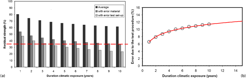
a Schematic representation of total uncertainty which should be taken into account for design purposes and b evolution of test procedure uncertainty

These strength predictions were then used to design a simple application: a self-bearing sandwich wall panel with a polyurethane foamed core (40 kg m⁻³) and a TRC composite faces (material combination VUB-comp-OPCII-R, with a random 2D fibre volume fraction of ∼9%). The panel is designed to be subjected to dead weight and a wind load of 1 kN m⁻² following Ref. 27. An element with a span of 2·4 m is considered. The core material is assumed to behave in a linear elastic manner in shear, up to a shear stress of 33% of the failure shear stress (or 0·2 MPa as previously obtained in Ref. 28). A shear stiffness of 8 MPa was taken for the core material.28 In compression, the faces are designed to behave in a linear elastic manner until failure. An average stiffness E_c1 of 23 GPa is assumed. The design failure stress in compression is 40 MPa. In tension, the material is characterised by a highly non-linear behaviour, which can be simplified to a bilinear behaviour. The corresponding material parameters are given in Fig. 5, with an average tensile strength of 14 MPa.

Figure 5

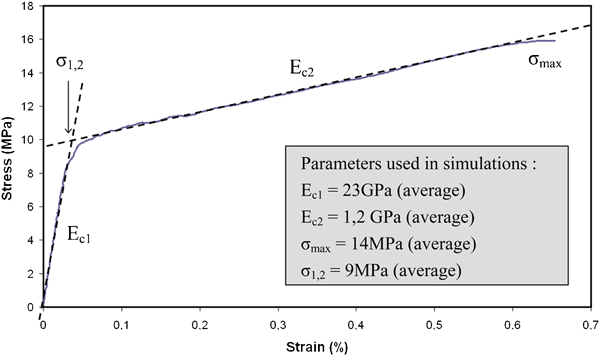
Typical tensile stress–strain behaviour of material combination under study

The design of the wall panel requires choosing a constant core thickness and allowing the face thicknesses to vary incrementally, with a size step of 1 mm (corresponding to the thickness of one lamina, i.e. one textile layer impregnated by concrete). The necessary minimum face thickness (both faces are assumed to have the same thickness) is chosen from the results in order to satisfy the design criteria in the ultimate limit state (ULS) and the serviceability limit state (SLS):29 no failure (in ULS) may occur, and deflections (in SLS) need to be limited to span/250.

A finite element program (ANSYS, version 11.0) is used, with the element ‘Shell 91’ to design the sandwich panel. The activated sandwich option allows the implementation of the sandwich theory (in order to calculate element stiffness and evolution of the stresses along the thickness of the element).

The calculations lead to the thicknesses given in Table 9. Five material options were studied:

non-aged 1: using the initial average material tensile strength of 14 MPa

ii.

non-aged 2: including the material uncertainty of 26·5%, thus a tensile strength of 10·3 MPa

iii.

aged 1: including only the material degradation of 40%, thus a residual tensile strength of 8·4 MPa

iv.

aged 2: including in addition the material uncertainty of 26·5%, thus a residual tensile strength of 4·7 MPa

aged 3: including the total uncertainty of 39·9%, thus a residual tensile strength of 3·1 MPa.

Table 9

Resulting face thicknesses for self-bearing sandwich wall elements with a span of 2·4 m (ANSYS)

Sandwich panel face thicknesses/mm
	Core thickness/mm
	50	60	75	100
Non-aged 1	3	2	1	1
Non-aged 2 (including material uncertainty)	3	2	1	1
Aged 1	3	3	2	2
Aged 2 (including material uncertainty)	4	4	3	3
Aged 3 (including material and test procedure uncertainty)	7	6	5	4

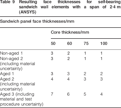
The highlighted areas within Table 9 correspond to results for which the SLS criterion is critical. For all other results, the ULS criterion is more important for the dimensioning (more precisely, the tensile strength of the faces). When analysing the results, it becomes clear that, in the unaged state, all the calculations are dominated by the SLS criterion, while the ULS criterion is critical for nearly all cases using the aged material. When comparing the results obtained for the three aged options, it also becomes clear that omitting the uncertainty on the material and/or the test procedure might result in seriously under dimensioned structural elements.

Conclusions

This paper presents several novel approaches for the analysis of GRC accelerated aging tests. First, the determination of the best approximating model was addressed using a statistical model selection method (the AIC). The application of this method on a substantial series of accelerated aging tests showed that the best approximating model in many cases differs from the best fitting model. A cost function approach, as opposed to a sum of squares based approach, should be used for the fitting of strength durability models to accelerated aging data series. Model selection is highly dependent on the material combination, type of specimen and testing procedure used. A single best approximating strength durability model valid for all datasets could not be found.

Second, a theoretical approach was presented that enables the user to check the reliability of the model selection. In some datasets, selection of the correct model can be impaired by non-robust experimental details. For the specific case presented in this paper, the number of specimens used to construct the averaged data points was insufficient. In other situations, however, different factors (such as the total number of data points or the duration of the test scheme) might also impede the model selection. The importance of a check on the reliability of the model selection for any given accelerated aging dataset was clearly demonstrated.

The third part of this paper presented a method for the determination of the uncertainty on a strength prediction based on accelerated aging testing. This method not only takes into account material uncertainties but also uncertainties that are directly related to the specificity of accelerated aging testing and modelling. This uncertainty due to the test procedure was found to be a complex product of the following:

the specific test scheme used

ii.

the number of specimens for each individual data point within the dataset

iii.

the scatter present on the experimental data

iv.

the type of model used.

The total uncertainty in strength predictions was found to generally lie between 30 and 40% of the initial, unaged strength of the material. For the datasets studies, the material uncertainty was established to be between 20 and 30%, and the test procedure uncertainty between 9 and 20%, of the initial strength of the material. The implications of this total uncertainty on strength predictions, and thus on the design of structural applications, was also briefly addressed. It was found that, for specific applications exposed to outdoor weathering, excluding the uncertainty on the test procedure in the design might lead to ill designed structures with a considerably reduced lifespan. As an example, a structure initially designed to withstand 10 years of Belgian outdoor weathering was found to potentially remain structurally safe for only 3 years.

Footnotes

Acknowledgements

Funding by the Flemish Fund for Scientific Research (FWO) under contract no. FWOAL320 is gratefully acknowledged. Funding by the Flemish Fund for Scientific Research (FWO) for a long stay abroad at the University of Warwick of the first author is gratefully acknowledged (FWO reference no. V4·074·07).

This paper is part of a special issue on Durability of composite systems

References

Van Itterbeeck

, Purnell

, Cuypers

, Wastiels

: ‘Study of strength durability models for GRC: theoretical overview’, Composites Part A , 2009, 40A, 2020–2030.

Orlowsky

, Raupach

, Cuypers

, Wastiels

: ‘Durability modelling of glass fibre reinforcement in cementitious environment’, Mater. Struct. , 2005, 38, 155–162.

Purnell

, Short

, Page

: ‘A static fatigue model for the durability of glass fibre reinforced cement’, J. Mater. Sci. , 2001, 36, 5385–5390.

Cuypers

, van Itterbeeck

, Wastiels

: ‘The effect of durability on the design of self-bearing sandwich panels with cementitious composite faces’, Proc. Conf. Brittle Matrix Composites 8, Warsaw, Poland, October 2006, Woodhead Publishing Limited, 99–108.

Purnell

, Cain

, van Itterbeeck

, Lesko

: ‘Service life modelling of fibre composites: a unified approach’, Compos. Sci. Technol. , 2008, 68, (15–16), 3330–3336.

Kim

, Wu

, Lin

, Li

, deLhoneux

, Akers

SAS

: ‘Micromechanics-based durability study of cellulose cement in flexure’, Cem. Concr. Res. , 1999, 29, 201–208.

Katz

, Bentur

: ‘Mechanisms and processes leading to changes in time in the properties of CFRC’, Adv. Cem. Based Mater. , 1996, 3, 1–13.

Mobasher

: ‘Modelling of toughness degradation and embrittlement in cement based materials due to interfacial aging’, Proc. 13th Conf. ASCE Engineering Mechanics Division, Baltimore, MD, USA, June 1999, ASCE.

Motulsky

, Christopoulos

: ‘Fitting models to biological data using linear and nonlinear regression: a practical guide to curve fitting’, 352; 2004, New York, Oxford University Press.

10.

Akaike

: ‘A new look at the statistical model identification’, IEEE Trans. Autom. Control , 1974, AC-19, 716–723.

11.

Bosdogan

: ‘Model selection and Akaike's Information Criterion (AIC): the general theory and its analytical extensions’, Psychometrika , 1987, 3, (52), 345–370.

12.

Burnham

, Anderson

: ‘Model selection and multimodel inference: a practical information-theoretic approach’, 488; 1998, New York, Springer.

13.

Rissanen

: ‘Modeling by shortest data description’, Automatica , 1978, 14, 465–471.

14.

Schwarz

: ‘Estimating the dimension of a model’, Ann. Stat. , 1978, 2, (6), 461–464.

15.

Sugiura

: ‘Further analysis of the data by Akaike's information criterion and the finite corrections’, Commun. Stat. A , 1978, 7A, 13–26.

16.

Hurvich

, Tsai

: ‘Regression and time series model selection in small samples’, Biometrica , 1989, 76, 297–307.

17.

McQuarrie

, Shumway

, Tsai

: ‘The model selection criterion AICu’, Stat. Probab. Lett. , 1997, 3, (34), 285–292.

18.

De Ridder

, Pintelon

, Schoukens

, Gillikin

: ‘Modified AIC and MDL model selection criteria for short data records’, IEEE Trans. Instrum. Meas. , 2005, 5, (53), 144–150.

19.

Orlowsky

: ‘Zur Dauerhaftigkeit von AR –Glasbewehrung in Textilbeton’, PhD thesis, RWTH-Aachen, Aachen, Germany, 2005.

20.

Purnell

, Short

, Page

, Majumdar

, Walton

: ‘Accelerated ageing characteristics of glass-fibre reinforced cement made with new cementitious matrices’, Composites Part A , 1999, 30A, 1073–1080.

21.

Litherland

, Oakley

, Proctor

: ‘The use of accelerated ageing procedures to predict the long term strength of GRC composites’, Cem. Concr. Res. , 1981, 11, 455–466.

22.

van Itterbeeck

, Cuypers

, Orlowsky

, Wastiels

: ‘Evaluation of the strand in cement (SIC) test for GRCs with improved durability’, Mater. Struct. , 2008, 41, 1109–1116.

23.

Schoukens

, Pintelon

: ‘Maximum likelihood estimation of errors-in-variables models using a sample covariance matrix obtained from small data sets’, Proc. 2nd Int. Workshop on ‘Total least squares and errors-in-variables modeling’, (ed. , Vanhuffel

), 59–68; 1997, Philadelphia, PA, SIAM.

24.

Andersons

, Joffeb

, Hojoc

, Ochiaic

: ‘Glass fibre strength distribution determined by common experimental methods’, Compos. Sci. Technol. , 2002, 1, (62), 131–145.

25.

Purnell

: ‘Interpretation of climatic temperature variations for accelerated ageing models’, J. Mater. Sci. , 2004, 39, 113–118.

26.

Orlowsky

, Raupach

: ‘Durability model for AR-glass fibres in textile reinforced concrete’, Mater. Struct. , 2008, 41, 1225–1233.

27.

BSI: ‘Actions on structures’, BS EN 1991-1, BSI, London, 2001.

28.

Cuypers

: ‘Analyses and design of sandwich panels with brittle matrix composite faces for building applications’, Doctoral thesis, Vrije Universiteit Brussel, Brussels, Belgium, 2002.

29.

BSI: ‘Design of concrete structures. Part 1-1 – General rules for buildings’, BS EN 1992-1-1, BSI, London, 2004.