Some effects of viscoelasticity on ability to model failure in composites

Abstract

The classical approach to modelling the thermomechanical response of composites employs a framework embodied within the concept of continuum mechanics. This approach may not always lead to success in that some failure mechanisms such as molecular scale phenomena may not be accurately captured by the continuum approximation. On the other hand, the continuum approach may be quite powerful and accurate for predicting failure in a variety of circumstances. For any continuum mechanics based approach to have hope of accuracy it is, however, necessary for that model to in some sense capture the physics of all of the cogent energy dissipative processes that are engendered in the actual application. The current paper takes the approach that failure due to fracture in viscoelastic composites can indeed be modelled entirely within the framework of continuum mechanics, but that in order to accurately predict failure due to fracture it is often necessary to deploy a model that is simultaneously cast within multiple length scales, each using the framework of continuum mechanics. This approach is taken for the simple reason that experimental observation suggests that in viscoelastic composites cracks form on the microscale, and these cracks eventually coalesce into macroscale cracks that cause the part to fail due to catastrophic facture. While predictions of these events may seem extraordinarily costly and complex, there are multiple structural applications where effective models would save considerable expense. The formulation for such an approach will be presented herein. This approach has been implemented into a finite element code and some example problems will be given in order to demonstrate the capabilities of the method.

Keywords

Multiscale modeling Failure Viscoelasticity Composites

Introduction

Many applications reveal that some inelastic heterogeneous solids undergo significant load and environmentally induced energy dissipation due to both bulk dissipation and the development of multiple cracks and/or voids. In viscoelastic materials, in particular, the energy dissipated in the bulk is governed not only by the material time scale but also by the loading time scale. The evolution of new internal boundaries can occur on multiple length and time scales, and often do not compromise the structural integrity due to the load redistribution and material inhomogeneities. Examples where this is sometimes the case include geologic salt, sea ice, polymer composites, tank armor, plastic ballistic explosives, and asphaltic pavement. In all of these heterogeneous materials experimentally based design methodologies are extremely costly, therefore suggesting the need for improved computational models.

One part of the traditional continuum mechanics approach that is often misused toward this end is in the deployment of a constitutive model. As a simple example, consider the case of an elastic constitutive model. Careful consideration of thermodynamics will lead to the conclusion that elastic materials cannot dissipate energy. Nonetheless, it is quite commonplace to see a linear elastic analysis utilised to predict failure of a structure. Sometimes this approach may turn out to be accurate despite the clear contradictory nature of the framework, but in many other cases the approach may be fatally flawed from the outset. In the latter case, it is sometimes possible to introduce sufficient improvement in a continuum based model by incorporating a viscoelastic constitutive model that the model is capable of making substantially improved predictions of failure.

In inelastic media, the problem of crack growth is particularly complicated by the fact that there are at least two competing energy mechanisms that occur essentially simultaneously whenever one or more cracks run: bulk material dissipation; and fracture energy. Thus, it can be quite difficult to separate the various sources of energy dissipation by experimental methods. Furthermore, due to material heterogeneities that can occur on multiple length scales, cracks can coexist over a broad range of length scales simultaneously, and the energy dissipated on these differing length scales can nevertheless be of the same order of magnitude. Finally, since material viscoelasticity by its very nature implies that there are governing time scales in the material behaviour, widely differing fracture events can be observed on differing time scales.

Due to the very complex nature of the problem, analytical solutions are most often precluded so that numerical solution techniques are preferred. Multiscale algorithms for problems of this type have until recently been untenable. This is due to the fact that the problem must be solved recursively on any and all length scales and at all locations in which the material microstructure is evolving in time. However, due to theoretical developments as well as the vast improvement in computing power of the last decade, it is now possible to solve some of such problems on two, three, and even four length scales by utilizing a single processor desktop computer. These solutions are obtained by using standard time marching multi-scale algorithms, linked by appropriate homogenization theorems,1^–6 permitting the prediction of the evolution of hundreds or even thousands of cracks simultaneously.

Multiscale models have been recently used for predicting the behaviour of composite materials7^–14 and some have even considered growing damage15, 16 and inertial effects.17 However, most of the multiscale models developed so far in the literature do not account for damage, inertial effects and viscoelasticity.

Multiscale modelling

Multiscale models can be generally viewed as constitutive models wherein the global constitutive behaviour of the heterogeneous material is determined simultaneously throughout the analysis based on the behaviour of the constituents and their interactions at the local scale. In most practical problems with local induced evolving microstructure, this is considerably advantageous, especially when formation and growth of cracks is considered, since the evolution of the microstructure is necessarily both spatially and time dependent.

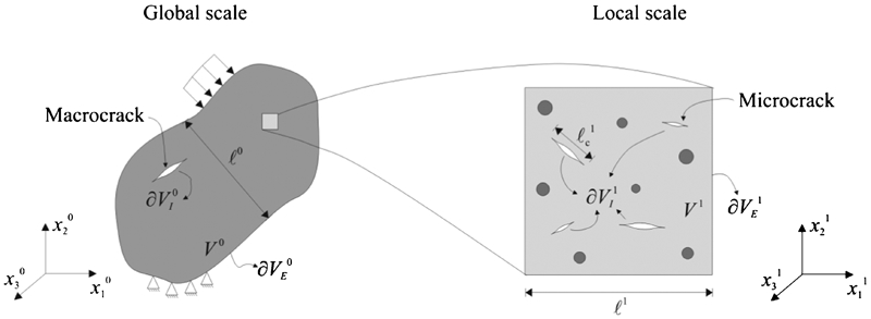
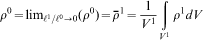
The purpose of multiscale models is to determine the locally averaged global constitutive behaviour of heterogeneous materials considering the geometry and constitution of the microstructure, which may include evolving cracks. Consider an object which is statistically homogeneous at the global scale but microscopically heterogeneous, as shown in Fig. 1, where the microstructure may contain inclusions as well as growing cracks. In Fig. 1, superscripts refer to a scale index, where 0 refers to the global scale and 1 refers to the local scale, V^μ, and are the volume, external and internal boundary surfaces of scale μ respectively, is the length scale associated with scale μ and is the length scale associated with the cracks at scale μ.

Figure 1

Description of two scale problem

For the global object, the Initial Boundary Value Problem (IBVP) can be posed as follows:

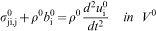
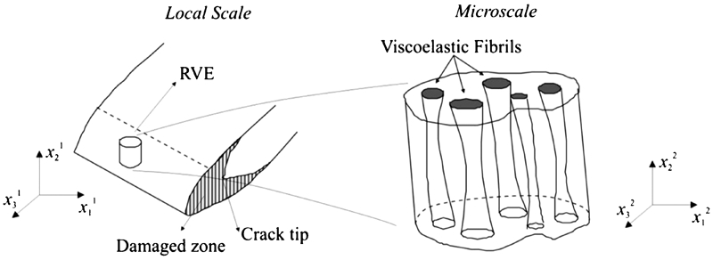
conservation of linear momentum (1) where is the Cauchy stress tensor, ρ⁰ is the mass density of the statistically homogeneous object, is the body force vector per unit mass, is the displacement vector and V⁰ is the volume of the object at the global length scale

ii.

conservation of angular momentum (2)

iii.

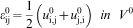
small strain–displacement relation (3) where is the infinitesimal strain tensor defined on the global length scale

iv.

constitutive equations (4) where is a functional mapping that accounts for history dependent effects, such as viscoelasticity, and is determined by locally averaging the response at the local scale.

If appropriate initial and boundary conditions are appended to equations (1)–(4), then a well posed Initial Boundary Value Problem (IBVP) will result. A fracture criterion, such as the Griffith criterion,18 can also be adjoined to the IBVP in order to allow modelling of new and existing cracks in the object. Note that equation (4) is not known a priori but can be determined during the multiscale analysis.

Now considering that the microscale is large enough such that continuum mechanics still applies, the local IBVP will look similar to the global one, but some assumptions are made in order to simplify the problem. For practical reasons, it is assumed that the global length scale is much larger than the local length scale (5) This assumption simplifies the connecting (homogenisation) relationships between the global and local scales. Moreover, it is assumed that the length scale associated with cracks at the local scale , is much smaller than the local length scale, and these cracks are homogeneously distributed at the local scale, thus mitigating statistical inhomogeneity on the local scale (6) Finally, as may be observed in many practical applications, it is also assumed that the length of the wave propagating on the global scale is much larger than the local scale length (7) Therefore, the local IBVP can be approximated as a quasi-static problem given by:

conservation of linear momentum (8)

ii.

conservation of angular momentum (9)

iii.

small strain–displacement relation (10)

iv.

constitutive equations (11) where in the case of the local scale, it is assumed that is known a priori, for all constituents.

fracture criterion (12) where is the fracture energy release rate at the local scale and is the critical energy release rate of the material. The index i refers to the mode of fracture.

Connecting local to global scale

Once the global and local IBVP have been posed, it is necessary to establish some relationship connecting both length scales. One way to link the local scale field variables to the global scale counterparts is via the use of mean fields, thus resulting in homogenization principles.

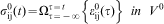
In analogy with continuum mechanics, one can use the assumption of to prove the strain tensor on the global length scale as the external boundary average of the displacements on the local length scale (13) where is the external boundary of the local length scale and is the outward unit normal vector to this external boundary surface.

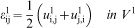
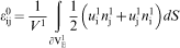
One can also show that6 (14) where is the volume averaged strain on the local length scale and is the internal boundary average of displacements on the local length scale, which are given by (15) (16) where is the internal boundary of the local length scale and is the outward unit normal vector to this internal boundary surface.

Note that can be regarded as an averaged damage quantity, since it is computed over the internal boundaries of the local length scale, including the cracks.6

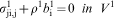
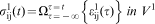
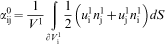
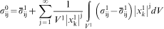
Now consider the following mathematical expansion for the global length scale stresses in terms of the local stresses (17) where is the volume averaged stress at local scale, which is given by (18) and the terms within the summation in equation (17) represent higher order area moments of the stress tensor.

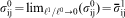
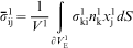
One can show that the assumption of leads to the following conclusion (19) One can also show, by means of the divergence theorem and equation (8), that (20) where the right hand side of the above is the external boundary averaged stress. Note that the boundary averaged stress is actually physically more palatable than the volume averaged stress, as it is commensurate with the original definition of stress, as defined by Cauchy,19 to act on a surface.

Using similar arguments, one can also show that (21) The use of equation (19) is termed a mean field theory because the higher order area moments of the local scale stresses in equation (17) are dropped and the global analysis is performed only in terms of the mean stress. In cases wherein there is a localisation process induced by damage or large strain gradients, some higher order terms in equation (17) will not be negligible and the mean field theory is no longer accurate. In this case, a non-local approach, including the non negligible terms in equation (17), or even a full field analysis performed simultaneously on all length scales may be necessary in order to obtain the desired degree of accuracy. Kouznetsova20 presents a second order computational homogenization scheme that accounts for the effects of strain gradients on the local scale. The necessity for accounting for localisation processes may be monitored by calculating the higher order terms in equation (17) for the local scale after each time step during the analysis. Once the higher order terms become non-negligible, one may decide to halt the analysis or continue the analysis with the awareness that its accuracy may be compromised.

Finally it is necessary to establish a constitutive relationship at the global length scale based on the constitution of the local scale. This can be done by direct substitution of the local scale constitutive equation, equation (11), into the volume average of stresses, equation (19). In multiscale analysis, however, there is no need to determine the global scale constitutive relation a priori, since it is determined concurrently as the analysis is performed.

In principle, the approach herein described can be applied on as many (continuum) length scales as necessary in order to solve complex problems. However, the limits of continuum scales for typical structures in nature (10⁻¹⁰m <λ<10³m), and the requirement that the length scales be broadly separated, as given by inequalities (5)–(7), lead to the conclusion that only about five, or perhaps six, length scales are practically possible. On the other hand, depending on the complexity of the given problem, only about three scales are computationally practical with current computer capabilities. Fortunately, there are few problems of current technological significance that require more than about three computational scales. Allen and co-workers have been able to obtain solutions on a desktop computer by this technique using as many as four length scales simultaneously, although it must be admitted that two of these scales were analytical.21

Crack modelling at local length scale

Crack propagation is herein modelled by using a cohesive zone model because this type of fracture mechanics model is more convenient to be utilized in computational algorithms and for modelling multiple cracks simultaneously. More specifically, we use the micromechanical viscoelastic cohesive zone model developed by Allen and Searcy.22

Cohesive zone models have been introduced by Dugdale23 and Barenblatt.24 The main shortcomings of cohesive zone models are essentially related to the inability to measure directly the material parameters necessary to characterise a particular cohesive zone model and to the fact that cohesive zone models are normally deployed in such a way that it is necessary to know where the crack will propagate a priori. The main advantages are that cohesive zone models are quite conveniently deployable into a finite element code and they can be formulated in such a way that the fracture phenomena in some media, especially inelastic, can be captured more accurately than can the Griffith criterion. For example, it is often observed in viscoelastic media that the critical energy release rate required for crack extension is rate dependent.

Allen and Searcy22, 25 have developed a cohesive zone model for viscoelastic media that is formulated in such a way that the material parameters required to characterize the cohesive zone model can be obtained directly from microscale experiments. Furthermore, this model is inherently two scale in nature in that it utilizes the solution to a microscale scale continuum mechanics problem, together with a homogenisation theorem to produce a cohesive zone model on the next larger length scale. The model has also been shown to be consistent with the fact that the cohesive zone requires a nonstationary critical energy release rate in order for a crack to propagate.26^–28

This model has already been well reported in the literature and will only be briefly reviewed here. As shown in Fig. 2, the cohesive zone is postulated to be represented by a fibrillated zone that is small compared to the total cohesive zone area. The length scale of this IBVP is one length scale below that of the smallest local scale required in the multiscale problem.

Figure 2

Depiction of micromechanical viscoelastic cohesive zone model22

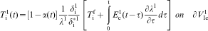
The solution to this IBVP has been obtained and homogenised,22 thus leading to the following traction–displacement relation in the cohesive zone (22) where is the uniaxial viscoelastic relaxation modulus of the undamaged cohesive zone material, is the part of the internal boundary on which cohesive zones are active, is the crack opening displacement vector in the coordinate system aligned with the crack faces, is a material length parameter, λ¹ is the Euclidean norm of the crack opening displacement vector, is the value of traction at which the cohesive zone initiates, and α(t) is the damage parameter, which in this case degenerates to a scalar, defined by (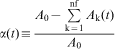23) where A₀ is the undamaged plan form cross-sectional area of a representative area of the cohesive zone, A_k(t) represents the cross-sectional area of the kth fibril, and nf is the number of fibrils contained in the representative area. It can be seen that when all of the fibrils in a representative area fracture, the damage parameter α(t) goes to unity and the traction vector in equation (22) becomes zero, thereby inducing crack propagation. Note that the damage parameter α(t) is a natural byproduct of the homogenisation process linking the microscale to the next larger scale.

Although one can determine the evolution of α(t) experimentally, in the current paper, the damage evolution is assumed to follow a phenomenological law22, 28 given by (24) (25) where A and m are microscale phenomenological material constants.

Details about the time wise incrementalization of the viscoelastic cohesive zone model can be found in works by Allen and Searcy,29 Foulk et al.30 and Seidel.31 The incrementalisation of the bulk viscoelastic constitutive model can be found in works by Zocher et al.32

Since cohesive zone elements may introduce additional compliance to the finite element mesh prior to crack initiation and increase the maximum bandwidth of the stiffness matrix, the computational model presented herein uses an algorithm to automatically insert cohesive zone elements into the finite element mesh at the moment in time at which the criterion for cohesive zone initiation is satisfied. In this case, the initiation criterion is given by (26) For a given solution step, the traction vector is computed for every elemental edge sharing that node. Then, the traction vector for every edge in the mesh is checked against the crack initiation criterion equation (26). Finally, if the crack initiation criterion is satisfied for some edge node, this node is doubled and a cohesive zone element is then created for the new surface. It is also important to say that the Lagrange multipliers technique is used in order to apply displacement constraints in the cohesive zone so that node interpenetration is precluded. Besides, the algorithm herein used is not limited to quadratic elements.33 This approach has been successfully implemented into MultiMech, the unique two-way coupled multiscale finite element software including viscoelasticity and fracture for dynamic and quasi-static problems.

Multiscale algorithm for dynamic/impact problems

The multiscale model above described can be implemented into a computational algorithm to allow approximate solutions to complex problems containing multiple length scales with cracks growing simultaneously on the different length scales. The computer software herein utilized is MultiMech, the unique two-way coupled multiscale finite element software including viscoelasticity and fracture for dynamic and quasi-static problems. In MultiMech, a local scale finite element mesh is assigned for every integration point belonging to the selected global scale elements.

The basic difference from a standard FEM algorithm is that in MultiMech every time some information about the constitution of the global material is needed the software automatically solves a complex IBVP at the local scale.

It should be noted that MultiMech is fully parallelized and can significantly reduce computing time and guarantee efficient use of the computational power available for the solution of multiscale problems.

Example problems

This section presents the application of the unique two-way coupled multiscale computational model to the solution of illustrative multiscale IBVP's.

Homogenisation of viscoelastic fibre reinforced composites with cracks

Fibre reinforced composite materials have continuously found a broad range of structural applications, such as jet engine parts, pressure vessels, helmets and tank armor. The advantage of these materials is that one can, in some sense, design its microstructure in order to obtain the desired overall properties. Some researchers have shown that carbon fibre reinforced materials can show considerable time-dependent (viscoelastic) behaviour inherited from the matrix material.34 Furthermore, fibre reinforced composites are in general filled with voids and defects due to the manufacturing process and can also contain lots of microcracks initiated by service loading. The model herein developed is intended to be used in such applications where both viscoelasticity and microcracking are important.

Assume that the microstructure shown in Fig. 3 corresponds to the Representative Volume Element of an arbitrary fibre reinforced composite. The fibres diameter has been arbitrarily defined as 1·0 μm. The fibres Young's modulus and Poisson's ratio are 100 GPa and 0·3 respectively. The matrix viscoelastic material properties are given in Table 1, the matrix Poisson's ratio is assumed constant and equal to 0·3 and the viscoelastic cohesive zone parameters have been arbitrarily selected as , , A = 5·0 and m = 0·5. It is assumed that the cohesive zone relaxation modulus is the same as the bulk matrix material.

Figure 3

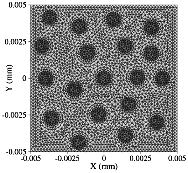
Initial geometry and FE mesh of RVE

Table 1

Viscoelastic properties of matrix material

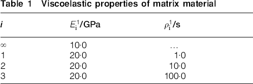
i	/GPa	/s
∞	10·0	…
1	20·0	1·0
2	20·0	10·0
3	20·0	100·0

Two other cases are also considered: one is the case where no cracks are allowed to initiate and grow, and the other is the case where the matrix material is assumed linear elastic with Young's modulus of 10 GPa ( ) and Poisson's ratio of 0·3. It is important to observe that all material properties herein used have been arbitrarily chosen.

For the loading conditions, biaxial displacements are applied to the boundaries of the RVE resulting in external boundary average strain rates of 1/s and 1/s in the vertical and horizontal directions respectively. The FE mesh contains initially no cohesive zone elements, which are automatically inserted into the mesh once the cohesive zone initiation criterion is satisfied.

Figure 4 presents the homogenized stress component as a function of time for the cases herein considered, from which one can see that accounting for viscoelasticity and microcracking can be very important. The analysis was stopped when the number of cohesive zone elements inserted in the mesh was big enough so that statistical homogeneity could not be guaranteed anymore. It is however important to distinguish cohesive zones (non-zero traction surfaces) from actual cracks (zero traction surfaces). Cracks are more likely to produce statistical inhomogeneity than cohesive zones because cracks produce strong discontinuities in the field variables, whereas the traction field is still assumed continuous across the cohesive zone. For these simulations, the authors were not able to accurately distinguish cohesive zones from actual cracks with the current post-processing capabilities, so that the analysis was stopped soon enough to avoid major cracks in the mesh.

Figure 4

Homogenised stress component as function of time

The evolution of component of the tangent constitutive tensor is shown in Fig. 5 from which one can see its dependence on the amount of accumulated damage. Results for the case where cracks are not allowed no initiate and grow are also shown along with the value of the volume average of the incremental (tangent) constitutive tensor, which is an upper bound value.

Figure 5

Component of homogenised tangent constitutive tensor

Figure 6 presents how all components of the homogenised incremental (tangent) constitutive tensor change as a function time. Note that the loading monotonically increases with time. Snapshots of the RVE for selected times are shown in Fig. 7 from which one can observed the amount of cracking occurring at each stage. These selected states are marked in Fig. 6 with vertical dashed lines so that one can correlate how the components of the homogenized incremental (tangent) constitutive tensor change as a function of crack density. Note that the internal boundaries shown in Fig. 7 can be either cohesive zones or actual cracks. As mentioned before, the current post-processing capabilities available to the authors cannot accurately distinguish cohesive zones from cracks, but from the stress state one can conclude that most of the internal boundaries are cohesive zones.

Figure 6

Components , , and of homogenised incremental (tangent) constitutive tensor as function of time

Figure 7

Snapshots of damage accumulated in RVE

The dependence of the history dependent stress tensor on the amount of accumulated damage is depicted in Fig. 8. Even though is a numerical quantity, the physical interpretation that can be drawn from the numerical results is that microcracking affects both instantaneous and history dependent response of the material, as expected.

Figure 8

Component of homogenised history dependent stress tensor as function of time

Multiscale modelling of viscoelastic fibre reinforced tapered bar

Consider the tapered bar shown in Fig. 9a as the global scale object of interest. Symmetry of geometry has been considered in order to minimise computational effort. Horizontal displacements are quasi-statically applied at the right end of the bar. Also assume that the local structure can be approximated by the RVE shown in Fig. 9b. A local structure of same initial geometry is used at all global scale integration points. Plane stress condition is assumed for both global and local scales. The fibre is again assumed linear elastic while the matrix is assumed linear viscoelastic. The arbitrarily chosen material properties used in this example are given in Table 2.

Figure 9

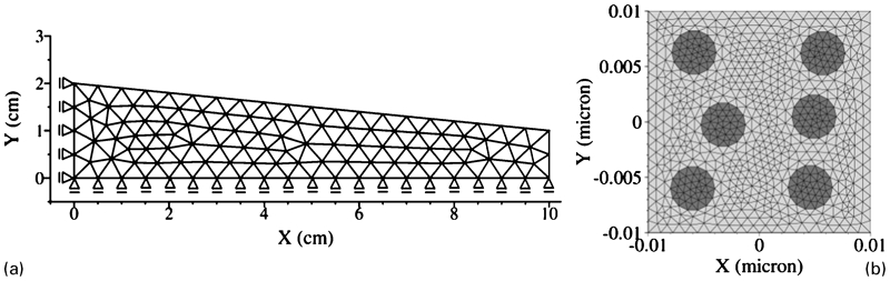
Geometry and FE mesh of tapered bar problem

Table 2

Material properties of local scale constituents

Bulk materials
Fibre		Matrix
ν ¹	0·3		ν ¹
E¹/MPa	550	i	/MPa	/s
		∞	350	…
		1	50	10⁻²
		2	50	10⁻¹
		3	50	10⁰
		4	50	10¹
		5	50	10²
		6	50	10³

Cohesive zones
	Matrix/matrix interfaces	Fibre/matrix interfaces
/nm	0·1	0·1
/nm	0·1	0·1
/MPa	40	30
/MPa	1000	200
A	0·25	0·5
m	1·5	1·5

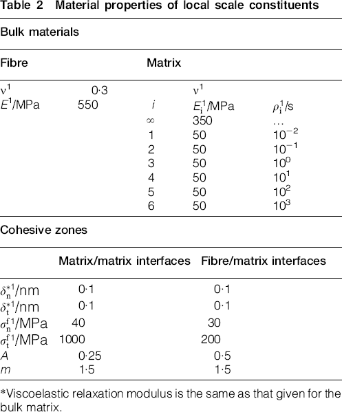
*Viscoelastic relaxation modulus is the same as that given for the bulk matrix.

As for the previous example problem, the local FE mesh initially does not contain any cohesive zone element, which is automatically inserted into the mesh once the cohesive zone initiation criterion is satisfied.

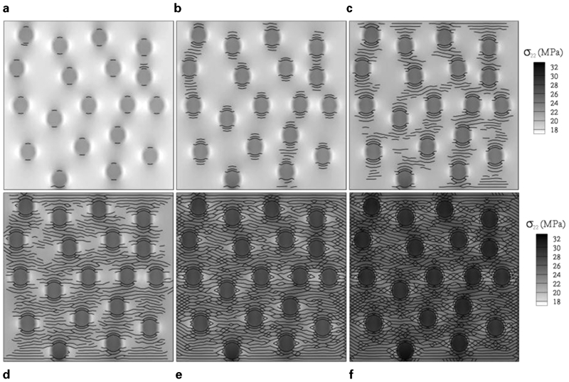
Figure 10 shows the contour of the component of the computed homogenized incremental (tangent) constitutive tensor as well as selected local structures at the end of the simulation, when the total applied tip displacement is of 0·74. The contour for the component of the stress tensor is shown for each selected local structure. Figure 11 presents how the homogenized modulus varies with the horizontal position along the symmetry line of the tapered bar. Values shown in the graph also correspond to the end of the simulation.

Figure 10

Contour of for global scale and contour of for local scale at different global positions

Figure 11

Component of homogenised tangent constitutive tensor as function of coordinate

As expected, one can observe from Fig. 10 that more damage is accumulated at regions of smaller cross-section, where stresses are concentrated. Consequently, is lower at smaller cross-sections (Fig. 11), once more damage has been induced at the corresponding local structures. It is once again important to note that the internal boundaries shown in Fig. 10 may not correspond to cracks, but to cohesive zones in fact.

It can be seen from Fig. 11 that there is a sudden drop in the stiffness at a certain position (approximately 6·8 cm). This sudden drop is produced by the automatic insertion of cohesive zone elements and the arbitrarily selected local scale geometry and material properties. Note that the stress field varies along , so that there will be a region in the global mesh for which the fracture criterion is not satisfied at the local scale and another region for which the fracture criterion is satisfied. Furthermore, for the current scenario, the state of stresses in the matrix material is approximately homogeneous so that most of the internal boundaries induced in the matrix are inserted at the same time step. The combination of all these factors thus produces a sudden drop in the stiffness and makes convergence more difficult to be achieved.

A further analysis of the results also reveals that the local structure is intact for <2·7 cm (see Fig. 11 and first local structure shown in Fig. 10), is slightly damaged for 2·7 cm< <6·8 cm (see Fig. 11 and second local structure shown in Fig. 10) and is very damaged for >6·8 cm (see Fig. 11 and third local structure shown in Fig. 10). The results also show that once most of the internal boundaries have been inserted, the evolution of the cohesive zone damage parameter α¹(t) governs the stiffness decrease, as expected.

Better results can be obtained if one considers statistical variation of the cohesive zone damage initiation stress throughout the mesh interfaces, simulating the existence of natural defects in the material. This feature is available in MultiMech but was not used in the present work for simplicity reasons. The use of larger (more fibres) statistically homogeneous RVEs and finer meshes could also improve the numerical results.

Conclusions

In this paper the authors have presented a methodology for predicting failure of viscoelastic composites that is formulated entirely within the framework of continuum mechanics. In order to capture the physics of failure due to fracture in such complex media a two-way coupled multiscale computational model has been employed. The intent of this approach is to accurately predict the energy dissipation that occurs due to the initiation and evolution of multiple microcracks. These microcracks are then predicted to evolve into macroscale cracks that eventually become unstable, causing failure of the structural component in question. We have shown how this process may be predicted utilizing an example problem herein.

The interested reader will find further research, including additional examples, in the references by the authors appended to this paper.

Footnotes

Acknowledgements

The authors are grateful for funding received for this research from the U.S. Army Research Laboratory under contract no. W911NF-04-2-0011. The first author also acknowledges former financial support from ANP, Agência Nacional do Petróleo, Gás Natural e Biocombustíveis, Brazil.

References

Eshelby

: ‘The determination of the elastic field of an ellipsoidal inclusion and related problems’, Proc. Royal Soc. A , 1957, 421A, 376–396.

Hill

: ‘Elastic properties of reinforced solids: some theoretical principles’, J. Mech. Phys. Solids , 1963, 11, 347–372.

Hashin

: ‘Theory of mechanical behavior of heterogeneous media’, Appl. Mech. Rev. , 1964, 17, 1–9.

Hill

: ‘A self-consistent mechanics of composite materials’, J. Mech. Phys. Solids , 1965, 12, 213–222.

Hill

: ‘Micromechanics of elastoplastic materials’, J. Mech. Phys. Solids , 1965, 13, 89–101.

Allen

, Yoon

: ‘Homogenization techniques for thermoviscoelastic solids containing cracks’, Int. J. Solids Struct. , 1998, 35, 4035–4054.

Allen

: ‘Damage evolution in laminates’, in ‘Damage mechanics of composite materials’, (ed. , Talreja

, ed), 79–114; 1994, Amsterdam, Elsevier.

Allen

: ‘Homogenization principles and their application to continuum damage mechanics’, Compos. Sci. Technol. , 2002, 61, 2223–2230.

Fish

, Shek

, Pandheeradi

, Shephard

: ‘Computational plasticity for composite structures based on mathematical homogenization: theory and practice’, Comput. Methods Appl. Mech. Eng. , 1997, 148, 53–73.

10.

Feyel

: ‘Multiscale FE2 elastoviscoplastic analysis of composite structures’, Comput. Mater. Sci. , 1999, 16, 344–354.

11.

Feyel

, Chaboche

J.-L

: ‘FE² multiscale approach for modelling the elastoviscoplastic behavior of long fibre SiC/Ti composite materials’, Comput. Meth. Appl. Mech. Eng. , 2000, 183, 309–330.

12.

Fish

, Shek

: ‘Multiscale analysis of composite materials and structures’, Compos. Sci. Technol. , 2000, 60, 2547–2556.

13.

Allen

, Searcy

, Soares

: ‘Multiscaling techniques for modeling damage evolution in asphaltic pavements’, Proc. Int. Conf. Comput. Exp. Eng. Sci., CD-ROM, Corfu, Greece, 2003.

14.

Souza

: ‘Modelo multi-escala para análise estrutural de compósitos viscoelásticos susceptíveis ao dano’, Master's dissertation, UFC, Fortaleza, Brazil, 2005.

15.

Allen

, Searcy

: ‘A model for predicting the evolution of multiple cracks on multiple length scales in viscoelastic composites’, J. Mater. Sci. , 2006, 41, 6510–6519.

16.

Talreja

: ‘Multi-scale modeling in damage mechanics of composite materials’, J. Mater. Sci. , 2006, 41, 6800–6812.

17.

Souza

, Allen

, Kim

Y.-R

: ‘Multiscale model for predicting damage evolution in composites due to impact loading’, Compos. Sci. Technol. , 2008, 68, 2624–2634.

18.

Griffith

: ‘The phenomena of rupture and flow in solids’, Philos. Trans. Royal Soc. Lond. A , 1920, 221A, 163–197.

19.

Cauchy

: ‘Recherches sur l’ équilibre et le mouvement intérieur des corps solides ou fluides, élastiques ou non élastiques’, Bull. Soc. Philom. , 1823, 9–13.

20.

Kouznetsova

: ‘Computational homogenization for the multi-scale analysis of multi-phase materials’, PhD thesis, TU-Eindhoven, Eindhoven, The Netherlands, 2002.

21.

Phillips

, Yoon

, Allen

: ‘A computational model for predicting damage evolution in laminated composite plates’, J. Eng. Mater. Technol. , 1999, 21, 436–444.

22.

Allen

, Searcy

: ‘A micromechanical model for a viscoelastic cohesive zone’, Int. J. Fract. , 2001, 107, 159–176.

23.

Dugdale

: ‘Yielding of steel sheets containing slits’, J. Mech. Phys. Solids , 1960, 8, 100–104.

24.

Barenblatt

: ‘The mathematical theory of equilibrium cracks in brittle fracture’, Adv. Appl. Mech. , 1962, 7, 55–129.

25.

Allen

, Searcy

: ‘A micromechanically-based model for predicting damage evolution in ductile polymers’, Mech. Mater. , 2001, 33, 177–184.

26.

Costanzo

, Allen

: ‘A continuum mechanics approach to some problems in subcritical crack propagation’, Int. J. Fract. , 1993, 63, 27–57.

27.

Costanzo

, Allen

: ‘A continuum thermodynamic analysis of cohesive zone models’, Int. J. Eng. Sci. , 1996, 33, 2197–2219.

28.

Yoon

, Allen

: ‘Damage dependent constitutive behavior and energy release rate for a cohesive zone in a thermoviscoelastic solid’, Int. J. Fract. , 1999, 96, 56–74.

29.

Allen

, Searcy

: ‘Numerical aspects of a micromechanical model of a cohesive zone’, J. Reinf. Plast. Compos. , 2000, 19, 240–248.

30.

Foulk

, Allen

, Helms

KLE

: ‘Formulation of a three-dimensional cohesive zone model for application to a finite element algorithm’, Comput. Meth. Appl. Mech. Eng. , 2000, 183, 51–66.

31.

Seidel

: ‘A model for predicting the evolution of damage in the plastic bonded explosive LX17’, Master's dissertation, Texas A&M University, College Station, USA, 2002.

32.

Zocher

, Groves

, Allen

: ‘A three-dimensional finite element formulation for thermoviscoelastic orthotropic media’, Int. J. Numer. Methods Eng. , 1997, 40, 2267–2288.

33.

Camacho

, Ortiz

: ‘Computational modelling of impact damage in brittle materials’, Int. J. Solids Struct. , 1996, 33, 2899–2938.

34.

Blassiau

, Bunsell

, Thionnet

: ‘Damage accumulation processes and life prediction in unidirectional composites’, Proc. Royal Soc. A , 2007, 463, 1135–1152.