Evaluation of temperature distribution in steel balls induced by friction generated during tribotest against diamond like carbon coatings

Abstract

Temperature rise in carbon steel (SUJ2-ASTM E52100) and stainless steel (SUS440C-ASTM 440C) balls sliding against diamond like carbon was evaluated using thermal simulation. On the premise that most of the friction energy was consumed as friction heat, the temperature distribution in the steel balls was simulated by ANSYS thermal conduction analysis using the friction energy measured by the ball on disc test. The interior temperatures of the steel balls were also monitored by a thermocouple during the tribotest. The simulation data, calibrated by the heat partition rate based on the Peclet number, were compared to the experiment data, and good accordance of both data was demonstrated.

Keywords

Steel DLC Energy input Friction heat Heat partition rate Temperature rise Thermal simulation

List of symbols

diameter of the contact area

specific heat

radius of the contact area

E _in

energy input

E_in(i)

energy input in segment i

friction force

F _i

friction force in segment i

gravity

mechanical equivalent of heat

thermal conductivity

L = υd/χ

Peclet number

M₁, M₂

layer 1, layer 2

normal load

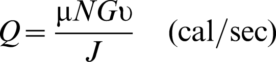
total heat supply rate

Q _B

heat supply rate to body B

Q _C

heat supply rate to body C

sliding distance

S _i

sliding distance in segment i

t₁, t₂

thickness of layer 1, layer 2

watt (joule/second)

density

friction coefficient

μ_i

friction coefficient in segment i

sliding velocity

χ = κ/ρc

thermal diffusivity

γ₁, γ₂

volume rate of layer 1, layer 2

θ _B

temperature rise on the contact area of body B

θ _C

temperature rise on the contact area of body C

θ _m

mean rise in temperature within the contact area

Introduction

Making fire by rubbing two wooden sticks together was the event that led humans to civilisation. Since the industrial revolution, friction heat has been a problem for engineering development. For diamond like carbon (DLC), it is important to consider the tribological behaviour of DLC based on the temperature rise at the contact area during sliding because researchers reported that the mechanical properties of DLC are degraded by annealing.^1–5 However, friction heat, such as the real maximum temperature on the scrubbed surface, is still poorly understood and has been investigated for years.^6–12

For the temperature rise at the contact area, Quinn¹³ reported that the ‘hot spot’ temperature was in excess of ∼700°C. Wang et al.¹⁴ demonstrated that the bulk surface temperature, corresponding to the transition from the mild wear mechanism to the severe wear mechanism, was ∼200°C for steel 52100. In fact, the measurement of the real temperature at the contact surface is very difficult, and many researchers have tried to measure the real maximum temperature on a sliding surface. Several methods, such as the infrared thermometer,^15,16 the embedded thermocouple method¹⁷ and the scrubbing materials that form a thermocouple,^18–22 have been tested. Bowden and Tabor rubbed a metal with transparent glass and detected the temperature of the contact area through the glass using an infrared thermometer.¹⁵ Shiozaki and Harada¹⁶ measured the cutting surface temperature of a milling tool using an infrared thermometer. The tribotest, using the two-body formed thermocouple, was introduced by Shore.¹⁸ He detected the electromotive force between the thermocouple materials, such as iron and constantan, while scrubbing them to evaluate the temperature rise on the contact surface. Bowden and Ridler¹⁹ measured the electromotive force between the thermocouple materials mounted in a pin on disc to estimate the temperature rise on the worn area. Furey²⁰ and Dayson²¹ evaluated the temperature rise of the worn surface between a constantan alloy ball and iron mating, comparing it to the Archard theoretical temperature.⁹ Uetz and Sommer²² implemented the tribotest of C45 iron and a constantan alloy and estimated that the worn area temperature was raised to 600°C. Their morphological analysis proved that the surface temperature of C45 iron reached nearly 800°C by observing the transformed martensite structure at the worn surface, although the electromotive voltage indicated less temperature 200°C below the transformed martensite temperature. It is recognised that even a direct measurement method cannot evaluate the real temperature of the scrubbed surface.

The temperature rise model of sliding bodies was proposed by Blok.^6,7 Blok introduced the ‘flash temperature’ concept and estimated the steady state, maximum temperature rise at the contact area with reference to the Peclet number. The Peclet number is a dimensionless number that is relevant to fluid flow theory, and its definition is the ratio of advective transport rate/diffusive transport rate. The Peclet number is normally used to evaluate the heat flow between two sliding bodies. He estimated the maximum temperature on the contact area under the assumption that the maximum temperature is independent of the sliding speed at a low Peclet number. For a high Peclet number, the maximum temperature equation was derived on the premise that the moving heat source was regarded as having an infinite length. Jaeger⁸ introduced the formula for the average temperature rise in terms of the Peclet number using the Bessel function.

The energy input induced by the friction between the surfaces is one of the most important parameters for determining the temperature rise. Generally, ∼95% of the frictional energy is transformed to heat, and the rest is dissipated during wear, noise and vibration.¹¹ Yamamoto et al.^23–26 researched the induced energy input by tribotesting and introduced the energy input measurement method using the friction coefficient sliding distance chart. He introduced the wear volume - energy input equation derived from the Holm–Archard equation and the wear rate equations with respect to the sliding velocity and the temperature.²⁵ Yamamoto et al. also proposed that the energy input was consumed by at least five tribological activities, including 1) wear energy, 2) friction heat, 3) elastic strain energy, 4) plastic deformation energy and 5) chemical energy.²³ They proved that the wear coefficient of the wear volume-energy input energy is equivalent to the energy consumption rate for wear to the energy input.²⁶

The ‘friction energy’, ‘dissipated energy’ and ‘energy input’ are equivalent in spite of their different names. ‘Friction energy’ emphasizes the energy consumed by tribological behaviour, and ‘dissipated energy’ implies a greater focus on energy consumption. ‘Energy input’ inleted in a power train transforms work, heat and friction energy. For tribotest, ‘energy input’ is the same amount of ‘friction energy’ because the tribometer is not intended to design for work. ‘Energy input’ in terms of the tribotest was because of the energy balance with the dissipated energy.

Figure 1 shows the energy balance between the energy input and the dissipated energy, where the thermal conductivity between the wear pair is the same. For frictional heat flow, because the heat partition rates differ due to the sliding conditions, such as the sliding velocity, contact area and sliding material's properties, the heat partition rate of the contacted two bodies has been discussed.¹²

Figure 1

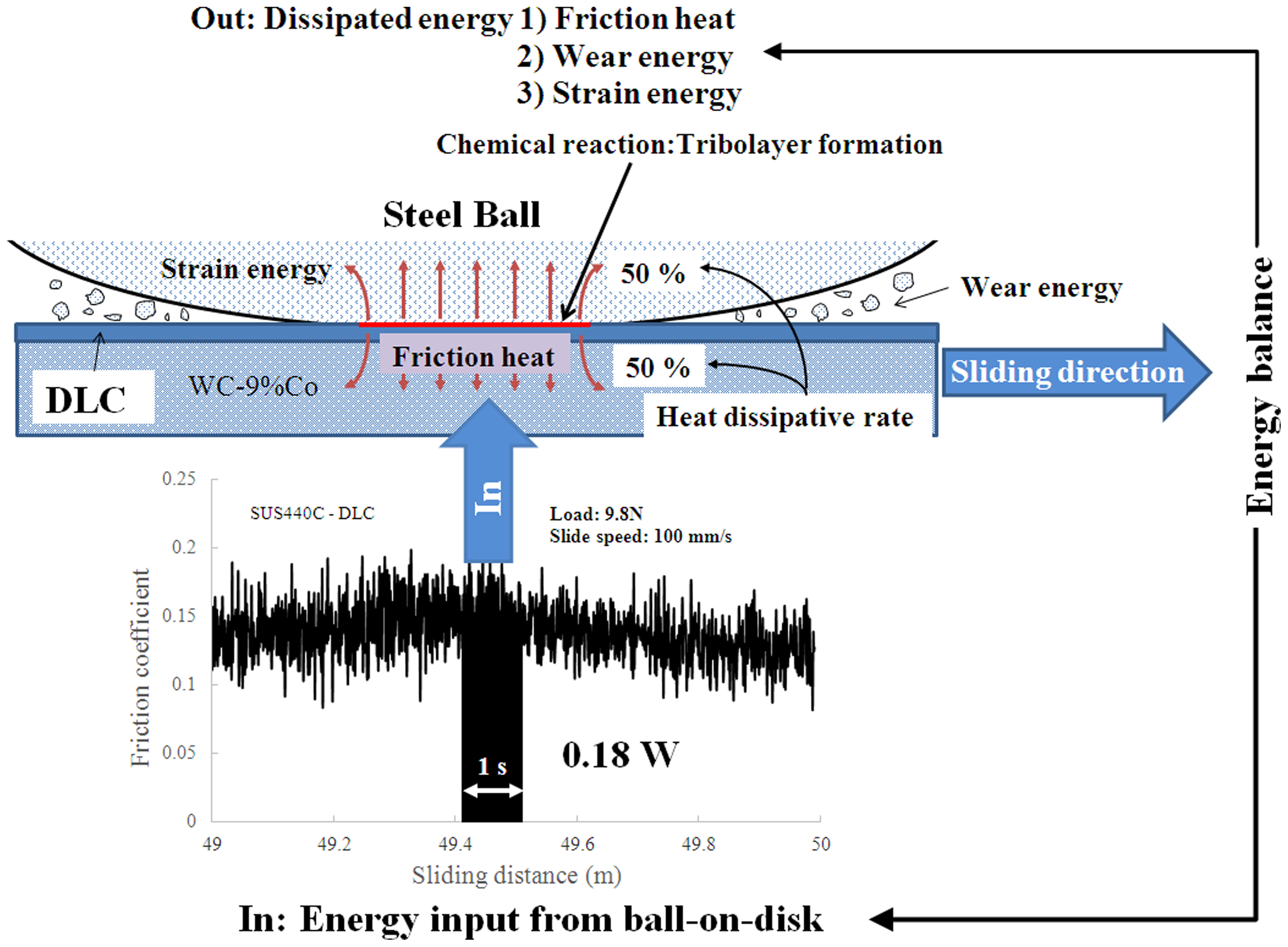
Energy balance between energy input and dissipated energy

Heat simulation is a useful and convenient tool to estimate the temperature rise at the rubbing surfaces. The heat distribution in the body can be calculated or simulated using the energy balance. Aghdam and Khonsari¹⁷ demonstrated the comparison of the friction temperature between the simulation and the experiment and indicated that the temperature simulation provided precise data.

In this study, the temperature distribution in the SUJ2 and SUS440C balls was simulated by ANSYS thermal conduction analysis on the premise that most of the friction energy was consumed as friction heat. For the temperature rise measurement, a thermocouple was mounted inside the steel balls at 0·3 mm above the contact area, and the inside temperature was monitored during the tribotest. The simulation and experimental data were compared and discussed in terms of the heat partition rate between the steel balls and the DLC.

Experiment

Diamond like carbon preparation

The DLC was derived from benzene (C₆H₆), as the gas source, using radio frequency (rf) plasma enhanced chemical vapour deposition on a WC–9%Co alloy for the tribotest.²⁴ After the substrate surfaces were cleaned by Ar bombardment for 5 min at a pressure of 0·05 Pa, an rf frequency of 13·56 MHz and an rf voltage of 0·25 kV, a silicon carbide layer, derived from hexamethyldisloxane C₆H₁₈OSi₂ gas at a pressure of 0·3 Pa and an rf voltage at 0·5 kV for 2 min, was deposited on the substrates as an intermediate layer. The DLC was deposited on the intermediate layer at 50°C by applying an rf voltage of 0·5 kV while feeding 15 sccm of benzene (C₆H₆) at 0·3 Pa. The thickness of the intermediate layer and the DLC were ∼30 nm and 1 μm respectively.

Temperature measurement in SUJ2 and SUS440C ball in tribotest

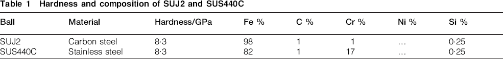
Because of the difficulty of drilling a φ 0·3 mm hole into the SUJ2 and the SUS440C balls, φ 5 mm pins, of which the contact side was shaped into a half sphere, were used for mating. Table 1 shows the hardness and the composite of SUJ2 and SUS440C. The depth of the hole was 0·3 mm above the contact point. The thermocouple (OMEGA TT-K-40 φ 80 μm) was settled at the bottom of the hole. The configuration of the temperature measurement system is shown in Fig. 2. The DLC was firmly mounted on the turn table of a ball on disc (RHESCA FRP-2100). A data logger (Graphtec GL-200L) was used to record the interior temperature at 100 ms sampling intervals with applied loads of 9·8, 19·6 and 29·4 N and a sliding velocity of 100 mm s⁻¹ without lubricants. The test environment was at room temperature (∼20°C), and the humidity was approximately 10–20%.

Figure 2

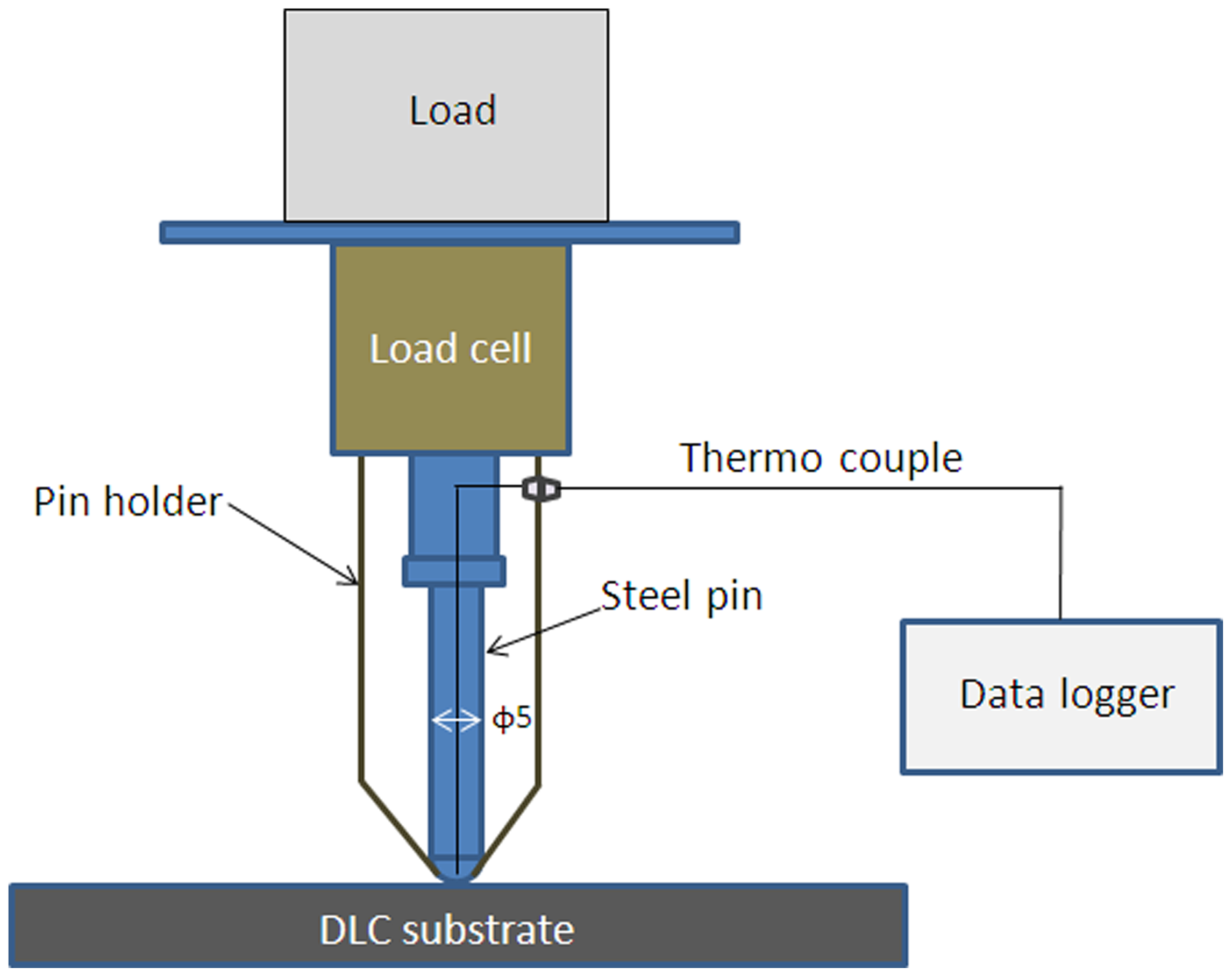
Schematic of friction heat measurement apparatus mounted thermocouple

Table 1

Hardness and composition of SUJ2 and SUS440C

Ball	Material	Hardness/GPa	Fe %	C %	Cr %	Ni %	Si %
SUJ2	Carbon steel	8·3	98	1	1	…	0·25
SUS440C	Stainless steel	8·3	82	1	17	…	0·25

Energy input measurement

The friction force F is measured by a load cell equipped in the ball on disc. The friction coefficient is calculated by the formula μ = F/N and was recorded at each sampling time. Because the friction force F_i is the value detected in the sliding distance S_i at the segment i, the input energy E_in(i) is the product F_i▪S_i. The total input energy E_in is obtained by equation (1) 1

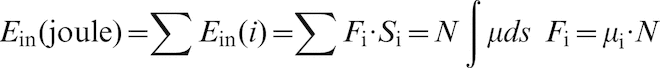
In practice, E_in was obtained based on the ΣF_i S_i in equation (1) using the CSV data logged friction force at each sampling time in the ball on disc system.

Temperature distribution simulation

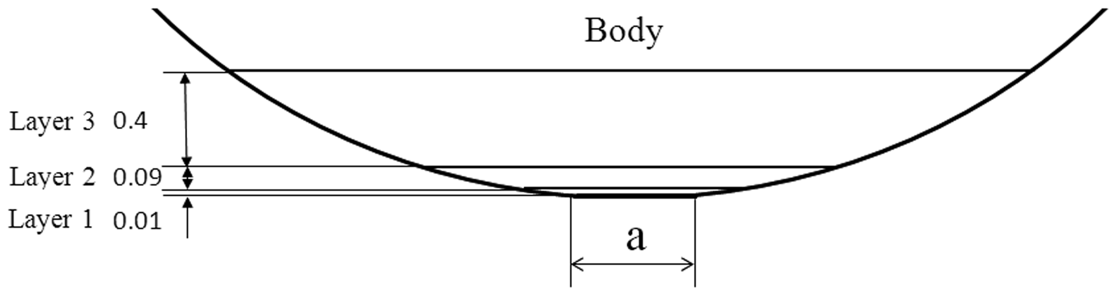
The temperature distribution in the steel ball was simulated by ANSYS. The size of the 3D sphere model was φ 4·8 mm, and the four sizes were designed with diameter a of 60, 90, 120 and 300 μm for the contact area. The expanded contact portion of the simulation model is depicted in Fig. 3. As shown in the figure, the bulk region, from the contact surface to 0·5 mm upward, was divided into three layers to apply different physical properties and the initial conditions. The thickness of the bottom layer (layer 1) was 0·01 mm and that of the second bottom layer was 0·09 mm. The third layer thickness was designed at 0·4 mm. The 3D model, of which the number of nodes and elements were 4870 and 1209 respectively, was simulated with a different energy input in watts under the condition that the heat flow to the sliding direction is negligible. Tables 2 and 3 show the initial parameters for the simulation of SUJ2 and SUS440C respectively.

Figure 3

Three-dimensional steel ball model for heat distribution simulation

Table 2

Initial condition for temperature distribution simulation in SUJ2 ball

Thermal conductivity/W m⁻¹ K⁻¹	Heat transfer coefficient/W m⁻¹ K⁻¹	Initial temperature/°C	Energy input/W
46 (SUJ2)	4·65×10⁻⁶	22 Layer 1	0·2 (at 4·9 N test)
15 (Fe₂O₃)		22 Layer 2	0·4 (at 9·8 N test)
		22 Body	0·8 (at 19·6 N test)
			1·2 (at 29·4 N test)

Table 3

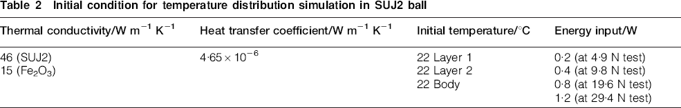
Initial condition for temperature distribution simulation in SUS440C ball

Thermal conductivity/W m⁻¹ K⁻¹	Heat transfer coefficient/W m⁻¹ K⁻¹	Initial temperature/°C	Energy input/W
24 (SUS440C)	4·65×10⁻⁶	22 Layer 1	0·09 (at 4·9 N test)
15 (Fe₂O₃)		22 Layer 2	0·18 (at 9·8 N test)
		22 Body	0·27 (at 19·6 N test)
			0·36 (at 29·4 N test)

Results

Temperature measurement result by thermocouple

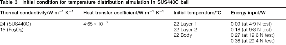
The temperature rise of SUJ2 and SUS440C at 0·3 mm above the contact surface was superimposed on the friction coefficient - sliding distance chart at a load of 29·4 N, as shown in Fig. 4a and b. The diameter of the contact surface after 200 m sliding was measured to be ∼400 μm. The inside temperature rises were synchronised with the friction coefficients. The temperature rise was not much higher than ∼5°C.

Figure 4

a temperature rise at 0·3 mm upward from contact area on SUJ2 during tribotest against DLC: load 29·4 N, sliding velocity 100 mm s⁻¹, and b temperature rise at 0·3 mm upward from contact area on SUS440C during tribotest against DLC: load 29·4 N, sliding velocity 100 mm s⁻¹

Temperature distribution simulation

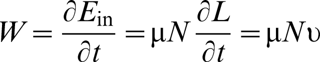
The temperature distribution in the steel balls was simulated by ANSYS with the input energy in watts on the contact surface. The energy input E_in is μNL, where the watts induced by the friction are also defined by the following equation 2 where t is time, and υ is the sliding velocity.

The energy input in watts can also be determined by the friction coefficient - sliding distance chart, as shown in the bottom chart of Fig. 1. Because the sliding velocity of the present tribotest was 100 mm s⁻¹, the watt was obtained by the product of the applied load and the area of the friction coefficient over a 100 mm distance. For instance, the input energy at 9·8 N for the SUS440C ball was ∼0·18 W, as shown in Fig. 1. Figure 5 shows the temperature distribution analysis result near the contact area of the SUJ2 ball with a contact diameter of 60 μm and an energy input at 1·2 W. The temperature distribution indicated that the maximum temperature occurred at the contact surface. The rapid temperature decrease inside the ball was exhibited. The bulk temperature over 0·5 mm from the contact point was the same as the initial temperature of the model due to the high thermal conductivity. Actually, the immediate temperature measurement of the steel balls, using an infrared thermometer, after the test verified that the post-temperature was the same as before the test.

Figure 5

Cross-section of temperature distribution around contact area of SUJ2: contact diameter: 60 μm, input watts: 1·2 W

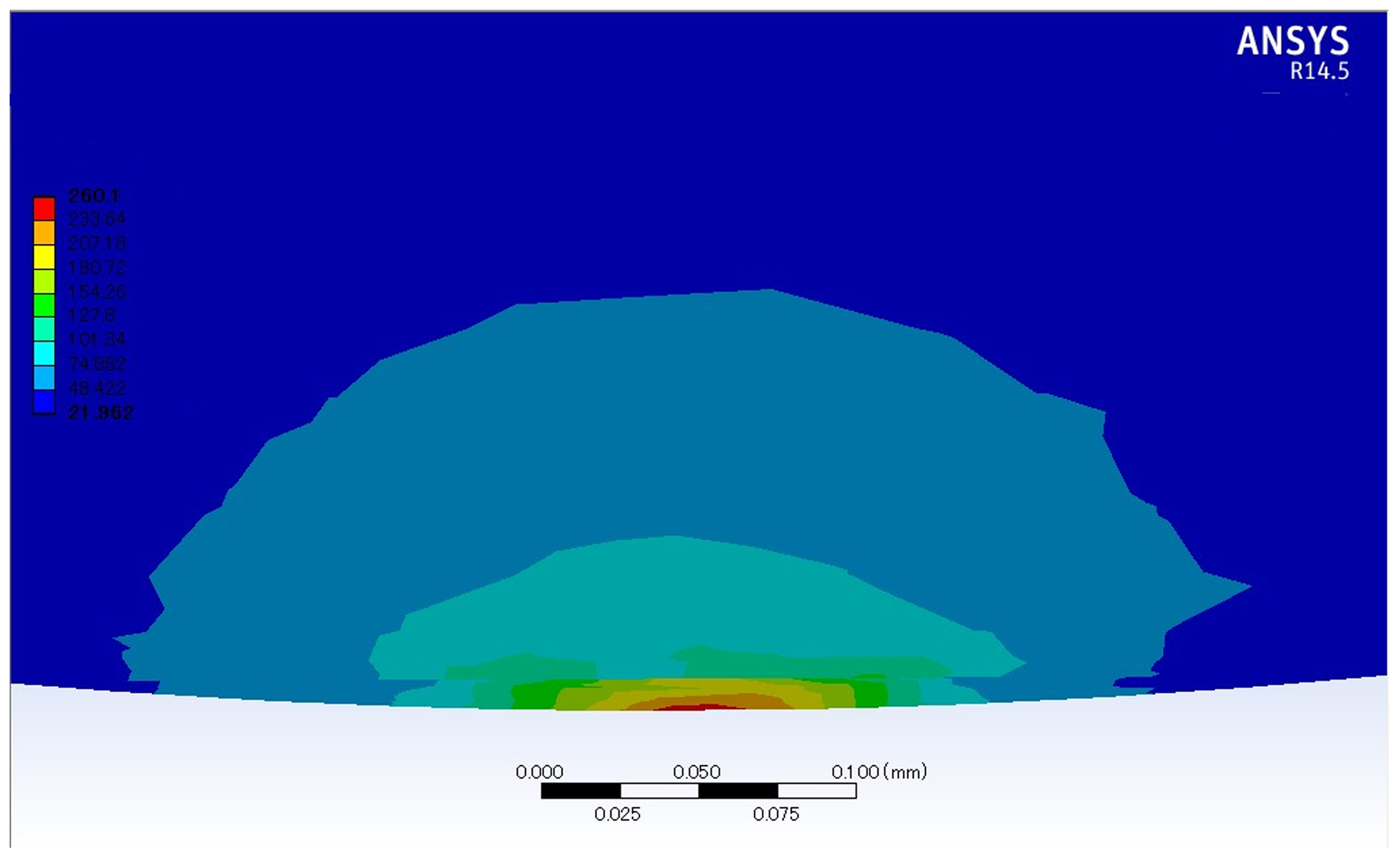
Figure 6a shows the maximum temperature dependence obtained by the simulation on the energy input in watts of the SUJ2 with various contact diameters. The maximum temperature was proportional to the energy input and inversely proportional to the diameter of the contact area.

Figure 6

a dependence of maximum temperature of SUJ2 on input energy, in watts, with different contact diameter obtained by ANSYS simulation (top layer: SUJ2 steel, contact diameter: 60, 90, 120 and 300 μm) and b dependence of maximum temperature of SUJ2 on input energy, in watts, with different contact diameter obtained by ANSYS simulation (top layer: Fe₂O₃, contact diameter: 60, 90, 120 and 300 μm)

The simulation result in the case where the top surface (layer 1) was iron oxide is shown in Fig. 6b. The maximum temperature of the energy input at 1·2 W, and for a contact diameter of 60 μm for the SUJ2 balls it was ∼580°C compared to 260°C without iron oxide.

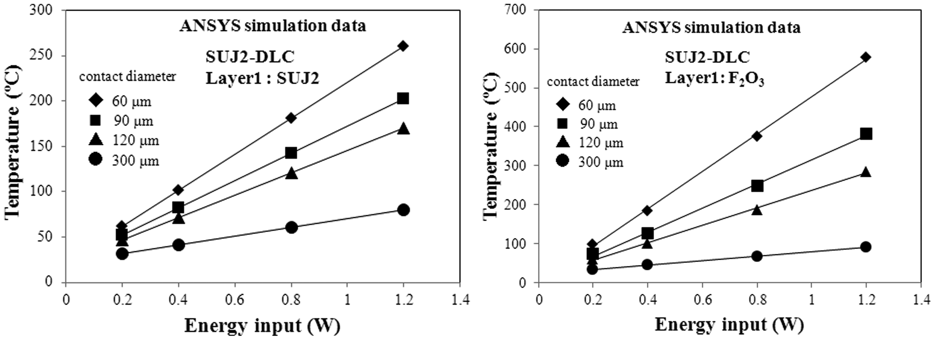
Figure 7a and b are the simulation results of the maximum temperature without iron oxide and with iron oxide as the top layer for the SUS440C balls. The maximum temperature of the SUS440C balls was approximately half that of the SUJ2 balls in each top layer mode.

Figure 7

a dependence of maximum temperature of SUS440C on input energy, in watts, with different contact diameter obtained by ANSYS simulation (top layer: SUS440C steel, contact diameter: 60, 90, 120 and 300 μm) and b dependence of maximum temperature of SUS440C on input energy, in watts, with different contact diameters obtained by ANSYS simulation (top layer: Fe₂O₃, contact diameter: 60, 90, 120 and 300 μm)

Discussion

Although the temperature rise was simulated under the assumption that all of the energy was consumed by the ball model, the energy input should be distributed between the steel ball and the DLC.

Archard studied the friction heat problem and introduced equations to estimate the interface temperature on the premise that friction heat should be applied to each body independently.⁹ The total heat supply rate Q is divided into Q_B and Q_C, as shown in equation (3) 3 where Q_B is the rate of heat supplied to the moving body B, and Q_C is the rate of heat supplied to the static body C.

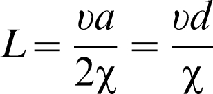
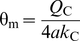
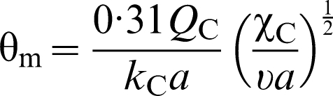
The heat partition rate of the two sliding bodies is dependent on the sliding velocity and the material properties. The Peclet number L, a non-dimensional parameter, is used to determine the heat partition rate. The Peclet number L is defined as 4 where υ is the sliding velocity, and a and d are the diameter and radius of the contact area respectively. The thermal diffusivity χ is defined as k/ρc, where k is the thermal diffusion coefficient, ρ is the density and c is the specific heat. Archard presumed that in the case where the sliding velocity is slow (L<0·1), the heat quantity was divided equally between the two bodies, namely Q_B = Q_C = 1/2Q. For high speed (L>100) sliding, the heat quantity is applied to body C, that is, Q_C = Q. He derived the temperature equations of the contact area in terms of the Peclet number. For a slow speed (L<0·1), the temperature equation is 5 where θ_m is the temperature of the contact area, and k_C is the thermal conductivity of body C.

For high speed sliding (L>5), the following equation was introduced 6

The temperature of the contact area for 0·1<L<5 was estimated graphically.

Archard also provided the temperature relationship between body B and body C, as shown below 7

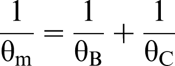
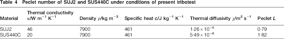
The total heat energy rate described in his paper was 8 where N is the load (g), G is the gravity (980 cm s⁻¹) and J is the mechanical equivalent of heat (4·18×10⁷ ergs cal⁻¹). Equation (8) is equivalent to the energy (joule s⁻¹) definition of equation (2) expressed by the MKS unit.

The Peclet numbers for SUJ2 and SUS440C calculated using the parameters of the stationary body are listed in Table 4.

Table 4

Peclet number of SUJ2 and SUS440C under conditions of present tribotest

Material	Thermal conductivity κ/W m⁻¹ K⁻¹	Density ρ/kg m⁻³	Specific heat c/J kg⁻¹ K⁻¹	Thermal diffusivity χ/m² s⁻¹	Peclet L
SUJ2	46	7900	461	1·26×10⁻⁵	0·79
SUS440C	20	7900	461	5·49×10⁻⁶	1·82

Bansal and Streator¹² derived a heat partition expression for static sphere body C and moving flat body B, which is the same situation as the ball on disc condition in the present study. Figure 8 shows the heat partition rate of the moving body as a function of the Peclet number based on their calculation. The heat partition percentage at Peclet 0·8 of SUJ2 and 1·8 of SUS440C were ∼48% (52% for the DLC) and 38% (62% for the DLC). Figure 9a and b shows the experimental data at 0·3 mm above the contact area, ANSYS data at the same location and ANSYS data calibrated by the heat partition rate of the SUJ2 and the SUS440C. The calibration data of SUJ2 and SUS440C were in good agreement with the experiment data.

Figure 8

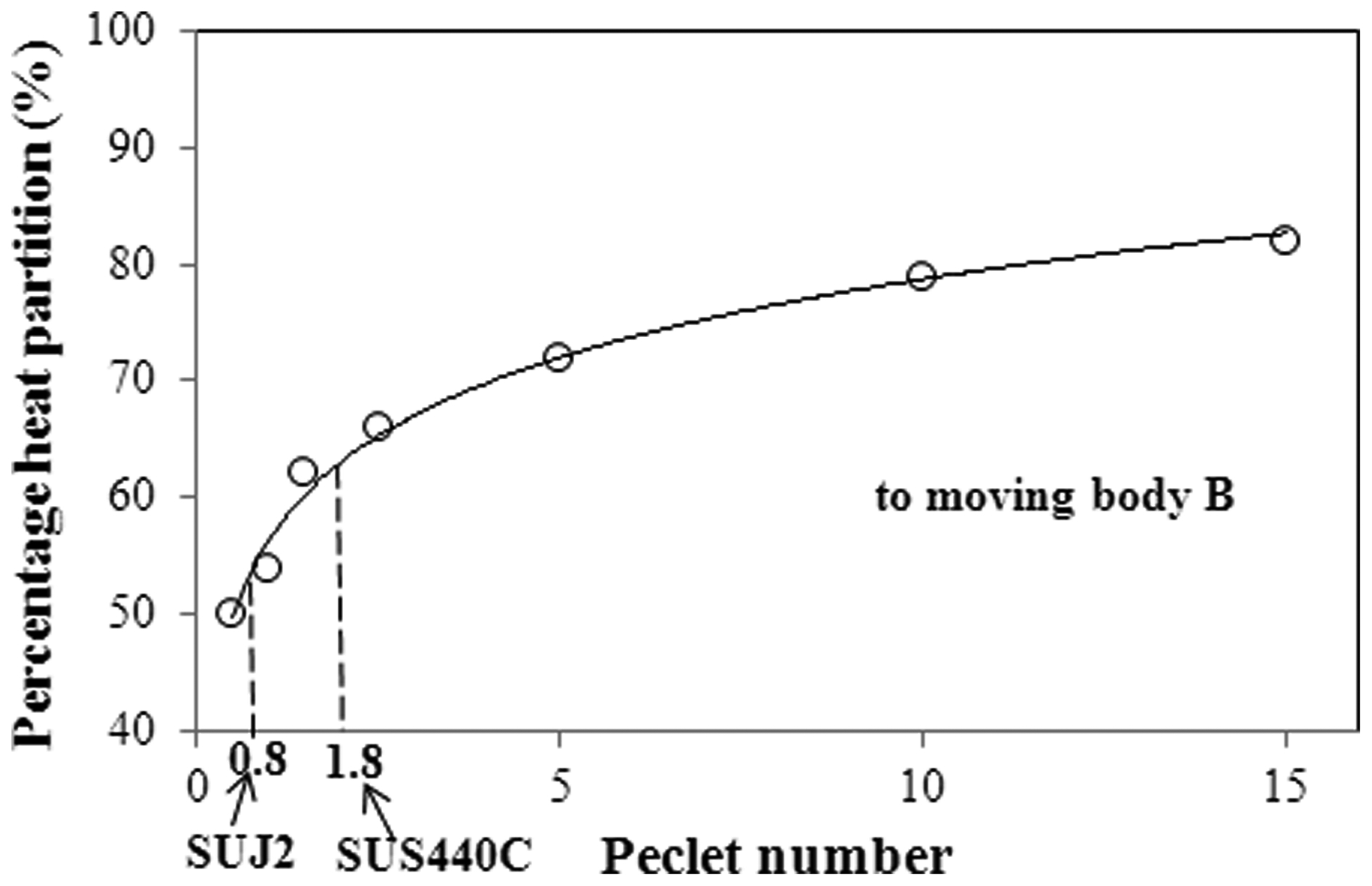
Variation, in percentage of heat partition, with Peclet number¹²

Figure 9

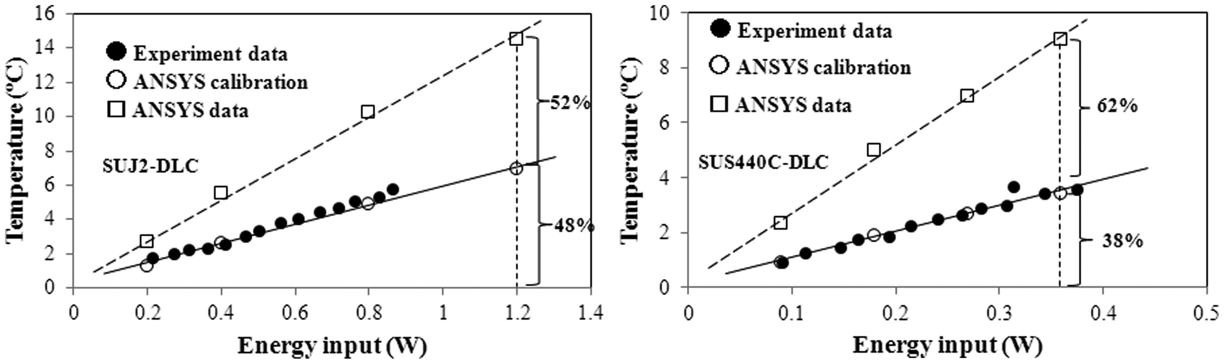
a temperature comparison between ANSYS and experimental data at 0·3 mm interior height for SUJ2 and b temperature comparison between ANSYS and experiment data at 0·3 mm interior height for SUS440C

The thermal conductivity of moving body B is also an important parameter to discuss with regard to the partition rate because the heat partition equation derived by Bansal and Streator was obtained in the case where the thermal conductivities of both bodies are equal. Generally, the thermal conductivity of the a-C:H type DLC is well <1 W m⁻¹ K⁻¹ due to the amorphous structure. However, the thermal conductivity of body B is a function of the configurations, which are a combination of a DLC film and a WC–9%Co substrate. According to heat transfer engineering, the thermal conductivity κ_total of the normal direction to the surface of the composite material, as shown in Fig. 10, can be expressed by the following equation on the premise that the interfacial thermal resistance was negligible 9 where κ₁ and κ₂ are the thermal conductivities of the configured material layer M₁ and layer M₂ respectively. γ₁ and γ₂ are the volume rates of M₁ and M₂ in the composite material respectively. Because both surface areas of the layers are equal, γ₁ and γ₂ are equivalent to thickness t₁ and t₂ for M₁ and M₂. The t₂ thickness at 0·5 mm was used because the thermal distribution evaluation obtained by the ANSYS simulation showed that the temperature over 0·5 mm was not changed to the initial temperature. The thickness and thermal conductivity of the DLC were 1 μm and 0·35 W m⁻¹ K⁻¹ (Ref. 27) respectively. The thermal conductivity of WC–9%Co was 67 W m⁻¹ K⁻¹. The thermal conductivity of the body B at 48 W m⁻¹ K⁻¹ was calculated using equation (9) and the parameters, which was approximately equal to that of SUJ2. Because the thermal conductivity of SUJ2 and the DLC/WC–9%Co system was nearly equal, good agreement between the calibrated simulation data and the experiment data was obtained. For SUS440C, the calibrated simulation data and the experiment data also fit, even though the thermal conductivity of SUS440C was lower than that of the DLC/WC–9%Co system. The Peclet number is normally used to evaluate the sliding velocity effect. If the sliding velocity is equal, the Peclet number dominates the thermal conductivity effect. Although the sliding velocity was equal in the present study, the Peclet number of SUS440C was larger than that of SUJ2 due to the lower thermal conductivity, which indicated the lower heat partition rate of the SUS440C body. As a result, the calibrated simulation and experiment data for SUS440C was equated.

Figure 10

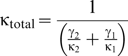
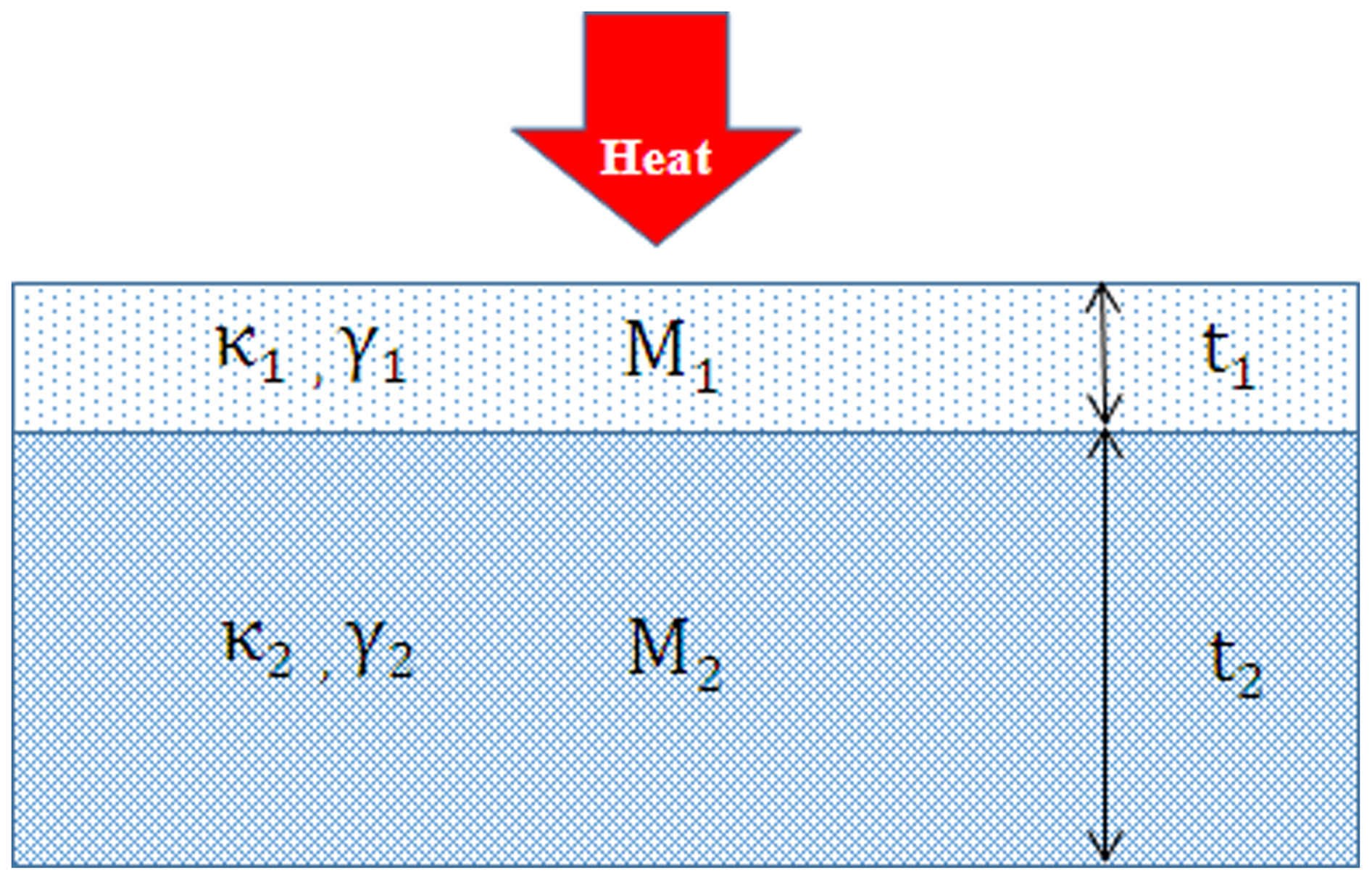
Thermal conductivity of composite material of DLC and WC–9%Co configuration

Archard's thermal Equations (5) and %(6) express that the contact surface temperature is decreased with a larger contact area diameter. Figures 6 and 7 show this phenomenon. Jaeger⁸ presumed that the existence of the iron oxide layer on the contact surface could cause a higher temperature rise on the oxide area. The temperature simulation result demonstrated a temperature rise with the iron oxide layer of ∼580°C at a 60 μm diameter and 1·2 W of input, the value of which was more than two-fold higher than without the oxide layer. The existence of iron oxide at the contact surface caused a higher maximum temperature because of the low thermal conductivity of iron oxide at 15 W m⁻¹ °C⁻¹. Yamamoto et al. showed that the iron oxide layer was formed at the head of the wear scar on the SUJ2 ball in the sliding direction.²³ The simulation result suggested that the highest temperature could be generated in the iron oxide layer portion.

Conclusion

The temperature distribution in the SUJ2 and SUS440C balls was simulated using the energy input, in watts, obtained from the friction coefficient - sliding distance data measured by the tribotest, and good agreement between the simulation data calibrated by the heat partition rate of the two bodies and the experimental data was demonstrated. The temperature simulation indicated that the temperature rise on the contact surface was the highest and that the temperature rise increased with the decrease in contact diameter and the existence of the iron oxide layer.

References

Wachter

and Cordery

: ‘Effects of post-deposition annealing on different DLC films’, Diamond Relat. Mater., 1999, 8, 504–509

Zhang

, Narumi

and Naramoto

: ‘Structure change of a hydrogenated carbon film upon heating’, J. Phys. Condens. Matter, 2001, 13, L475–L481

, Xu

, Wang

, Chen

, Zhou

and Liu

: ‘Annealing effect on the structure, mechanical and tribological properties of hydrogenated diamond-like carbon’, Thin Solid Films, 2006, 515, 2153–2160

Takabayashi

, Okamoto

, Sakaue

, Takahagi

, Shimada

and Nakatani

: ‘Annealing effect on the chemical structure of diamondlike carbon’, J. Appl. Phys., 2008, 104, 043512.

Wang

, Nie

and Hu

: ’Effect of thermal annealing on tribological and corrosion properties of DLC coatings’, J. Mater. Eng. Perform., 2013, 22, 3093–3100.

Blok

: ‘Theoretical study of temperature rise at surfaces of actual contact under oiliness lubricating conditions’, Inst. Mech. Eng., Proc. Gen. Discuss. Lubr. Lubr., 1937, 2, 222–235.

Blok

: ‘The flash temperature concept’, Wear, 1963, 6, 483–494.

Jaeger

: ‘Moving sources of heat and the temperature at sliding contacts’, Proc. R. Soc. New South Wales, 1942, 56, 203–224.

Archard

: ‘The temperature of rubbing surface’, Wear, 1958/59, 2, 438–455.

10.

Komanduri

and Hou

: ‘Analysis of heat partition and temperature partition in sliding systems’, Wear, 2001, 251, 925–938.

11.

Majcherczak

, Dufrenoy

and Berthier

: ‘Tribological, thermal and mechanical coupling aspects of the dry sliding contact’, Tribol. Int., 2007, 40, 834–843.

12.

Bansal

and Streator

: ‘A method for obtaining the temperature partition at the interface of sliding bodies’, Wear, 2009, 266, 721–732.

13.

Quinn

TFJ

: ‘The effect of ‘hot-spot’ temperatures on the unlubricated wear of steel,’ ASLE Trans., 1967, 10, 158–168.

14.

Wang

, Lei

, Yan

and Gao

: ‘Wear rate, frictional temperature, and energy consumption of steel 52100 with different microstructures during sliding,’ J. Phys. D, 1992, 25D, A165.

15.

Bowden

and Tabor

: ‘The friction and lubrication of solids’; 1950, London, Oxford University Press.

16.

Shiozaki

and Harada

: ‘Cutting edge temperature of face-milling cutter’, Sci. Pap. Inst. Phys. Chem. Res., 1962, 56, 209–215.

17.

Aghdam

and Khonsari

: ‘Prediction of wear in reciprocating dry sliding via dissipated energy and temperature rise’, Tribol. Lett., 2013, 50, 365–378.

18.

Shore

: ‘Thermoelectric measurement of cutting tool temperatures’, J. Wash. Acad. Sci., 1925, 15, 85–88.

19.

Bowden

and Ridler

KEW

: ‘Surface temperature of sliding metals’, Cambridge Phil. Sac. Proc., 1935, 31, 431–432.

20.

Furey

: ‘Surface temperatures in sliding contact’, ASLE Trans., 1964, 7, 133–146.

21.

Dayson

: ‘Surface temperatures at unlubricated sliding contacts’, ASLE Trans., 1967, 10, 169–174.

22.

Uetz

and Sommer

: ‘Investigations of the effect of surface temperatures in sliding contact’, Wear, 1977, 43, 375–388.

23.

Yamamoto

, Kawana

and Masuda

: ‘Tribological behaviour of stainless steel with respect to that of DLC in terms of energetic aspects’, Tribol. Mater. Surf. Interfaces, 2013, 7, (4), 161–167.

24.

Yamamoto

, Kawana

and Masuda

: ‘Tribological behavior of diamond-like carbon produced by rf-PCVD based on energetic evaluation’, Surf. Coat. Technol., 2013, 236, 457–464.

25.

Yamamoto

: ‘Tribological mechanisms of steels with respects to diamond-like carbon in terms of energy input’, Tribol. Trans., 2014, 57, 1001–1006.

26.

Yamamoto

, Egashira

, Kondoh

and Masuda

: ‘Evaluation of the wear energy consumption of nitrogenated diamond-like carbon against alumina’, Tribol. Lett., 2014, 55, 279–288.

27.

Alwi

, Kim

, Awang

, Rahman

and Krishnaswamy

: ‘Measurement of thermophysical properties of hydrogenated amorphous carbon films using picosecond thermoreflectance technique’, Int. J. Heat Mass Transfer, 2013, 63, 199–203.