Automated Cosmic Spike Filter Optimized for Process Raman Spectroscopy

Abstract

Despite the existence of various methods to remove cosmic spikes from Raman data, only a few of them are suitable for process Raman spectroscopy. The disadvantages of these algorithms include increased analysis time, low accuracy of spike detection, or reliance on variable parameters that must be chosen by trial and error in each case. We demonstrate a novel approach to detecting cosmic spikes in process Raman data and validate it using a wide range of experimental data. This new method features a multistage spike recognition algorithm that is based on tracking sharp changes of intensity in the time domain. The algorithm effectively distinguishes cosmic spikes from random spectral noise and abrupt variations of Raman peaks, allowing accurate detection of both high and low intensity cosmic spikes. The procedure is free from variable user-defined parameters and operates reliably in a fully automated manner with a wide range of time-series process Raman data sets containing more than 40 to 50 spectra.

Keywords

Raman spectroscopy Process analysis Data processing Cosmic spikes Outliers Automated correction

INTRODUCTION

The advent of multi-channel detectors such as charge-coupled devices (CCD) and photodiode arrays had a great impact on the development of Raman instrumentation by enabling much faster analysis.¹ However, these detectors are sensitive to cosmic rays that contaminate the recorded spectra with spurious spikes. These spikes have variable intensities and bandwidths and occur randomly in both time and frequency domains. The random nature of cosmic spikes makes it difficult to filter them out in an automatic and reliable manner. The need to remove cosmic spikes is widely recognized^2–10 and dictated by the data processing complications that they cause, especially when univariate analysis is used. Multivariate techniques such as principal component analysis can separate cosmic spikes from Raman peaks, but the principal components of higher orders often remain partially contaminated.

One way to remove cosmic spikes is to acquire two Raman spectra of the same sample. Because of the very low probability of two cosmic rays striking the same detector pixel in two sequential spectra, choosing the lowest intensity value recorded at each pixel or using more elaborate algorithms based on the same idea^4,5 results in a spike-free spectrum. This approach is widely used in the spike-filtering software supplied with many commercial Raman spectrometers. Although cosmic filters based on double acquisition are effective and conceptually simple, they double the analysis time and are prone to errors when identical sampling conditions cannot be provided for the consecutive spectra.

Alternative methods of automatic spike removal require hardware modification such as dividing the spectrograph slit into several tracks⁶ and analyzing the entire CCD image¹¹ to detect cosmic spikes. The utility of these methods is very limited due to the necessity of modifying the spectrometer or geometry of the collection fibers and incorporating post measurement data analysis with added detector noise from multiple tracks.

Several mathematical algorithms for cosmic spike detection and removal have been reported.^2,3,12,13 Their main disadvantage is an inability to simultaneously achieve full automation and high detection accuracy; this results from a dependence on variable parameters defined by the user and the requirement that cosmic spikes must be much narrower than Raman peaks (which is not always the case in practice). A number of mathematical algorithms have been developed for Raman imaging^{5,7,8,14,–16} but these are not suitable for other applications.

Process Raman spectroscopy is one application of the technique where existing cosmic filters do not provide satisfactory results. When the chemical composition of a reaction mixture changes rapidly and variable spectral background is present, double spectral acquisition is not appropriate and current mathematical algorithms do not provide the required speed, accuracy, and automation. One of the most well-established spike-removal algorithms for time-series Raman data, the UBS method,⁵ uses two variable parameters and is prone to misdetections when the profile of Raman spectra changes over time due to chemical changes in the sample. These misdetections cause disproportionate intensity changes of the most varying Raman bands such that intensities of some bands are reduced while other bands remain intact. The distortion of peak ratios caused by such modifications compromises valuable information in the Raman data. To the best of our knowledge, only two reported cosmic filters have been developed specifically for process Raman spectroscopy. In one of them,⁹ a statistical analysis based on second derivatives calculated along the sample (time) axis is used to distinguish cosmic spikes from smooth chemistry-induced spectral changes. Full neighboring spectra are used to correct the contaminated spectra. This algorithm has several disadvantages such as a reliance on two user-defined parameters, an inability to deal with heavily contaminated data sets caused by interferences in neighboring spectra, and a high risk of misdetections due to fundamental limitations of the absolute value of second spectral derivatives as the means of cosmic spike detection. The other method¹⁰ is based on a moving window approach^2,3,12,13 and cannot simultaneously provide full automation and high detection accuracy due to difficulties associated with detection of cosmic spikes that have bandwidths comparable with those of strong Raman peaks.

In the present work, we report a fully automated cosmic spike removal algorithm with no variable parameters and exceptionally high detection accuracy, the efficacy of which has been proven with a wide range of batch and continuous flow reaction data.

THE ALGORITHM

Detection of Cosmic Spikes. In process Raman spectroscopy, the spectral acquisition time and the time interval between acquisitions are usually chosen to be smaller than the characteristic reaction time. This is necessary to achieve sufficient temporal resolution for process understanding and modeling.

Within these conditions, intensities of the Raman bands change rather smoothly from sample to sample, reflecting gradual chemical changes in the reaction mixture. In contrast, a cosmic spike appears as an abrupt and considerable increase in signal at a random location in the spectrum. The probability of another cosmic spike occurrence at the same location in the following spectrum is very low so the increased signal usually falls back to the original baseline immediately. Such behavior is specific to cosmic spikes and is used to distinguish them reliably from smooth intensity variations caused by the chemical process.

Part of the present algorithm was designed to mimic the way we visually judge whether a spike on a Raman spectrum has a cosmic or chemical origin, based on random occurrence of unusually sharp spectral features.

The procedure devised for detecting cosmic spikes consists of the following steps:

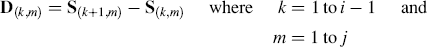
The initial Raman data set, comprising a series of consecutive spectra (e.g., Fig. 1a), denoted S_(i,j), where i and j are sample numbers and wavenumbers, respectively, is differentiated along the time (sample) axis at each wavenumber separately using a forward difference method:

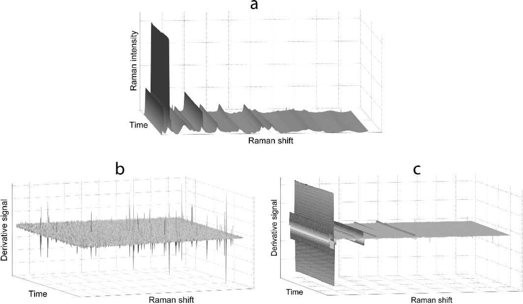
\begin{array}{l} D_{(k, m)} = S_{(k + l, m)} - S_{(k, m)} & where & k = 1 to i - 1 & and \\ m = 1 to j \end{array}

The last point (k = i) is assigned an average value of all preceding points to ensure that S and D have the same size; D_(i,j) shows step-wise signal changes from one sample to another. Figure 1b demonstrates that differentiating along the time axis levels out smooth chemical changes, making abrupt cosmic spikes more visible. This effect is not achieved when differentiating along the wavenumber axis (Fig. 1c).

At each wavenumber, the maximum and the minimum points in the D matrix are identified and temporarily removed from the data set to calculate standard deviations σ_(1,j) without these two points. A removed point is labeled as an outlier if its absolute value exceeds a threshold t_(1,j) proportional to the standard deviation σ (Fig. 2a). This threshold must be sufficiently high to minimize the probability of false positives, but not too high in order to detect all cosmic spikes. The signs of all outliers are recorded to be used later (see step 4). For explanatory purposes, the threshold value of 4σ was initially chosen. It will be shown later that the optimal value of threshold is independent of the spectra.

Step 2 is repeated independently for each wavenumber until the newly identified maximum and minimum values no longer exceed the threshold (Figs. 2b and 2c). The standard deviation values and corresponding thresholds are decreased after each iteration as new outliers are expunged from the data set. The final values of standard deviations for each pixel are saved and will be used later (see next section). Calculating the threshold without the outliers is necessary for maintaining high cosmic spike detection accuracy in heavily contaminated data sets because a single high-intensity cosmic spike can result in a significantly overestimated value of standard deviation that impedes detection of other less intense cosmic spikes at the same wavenumber (Fig. 2a).

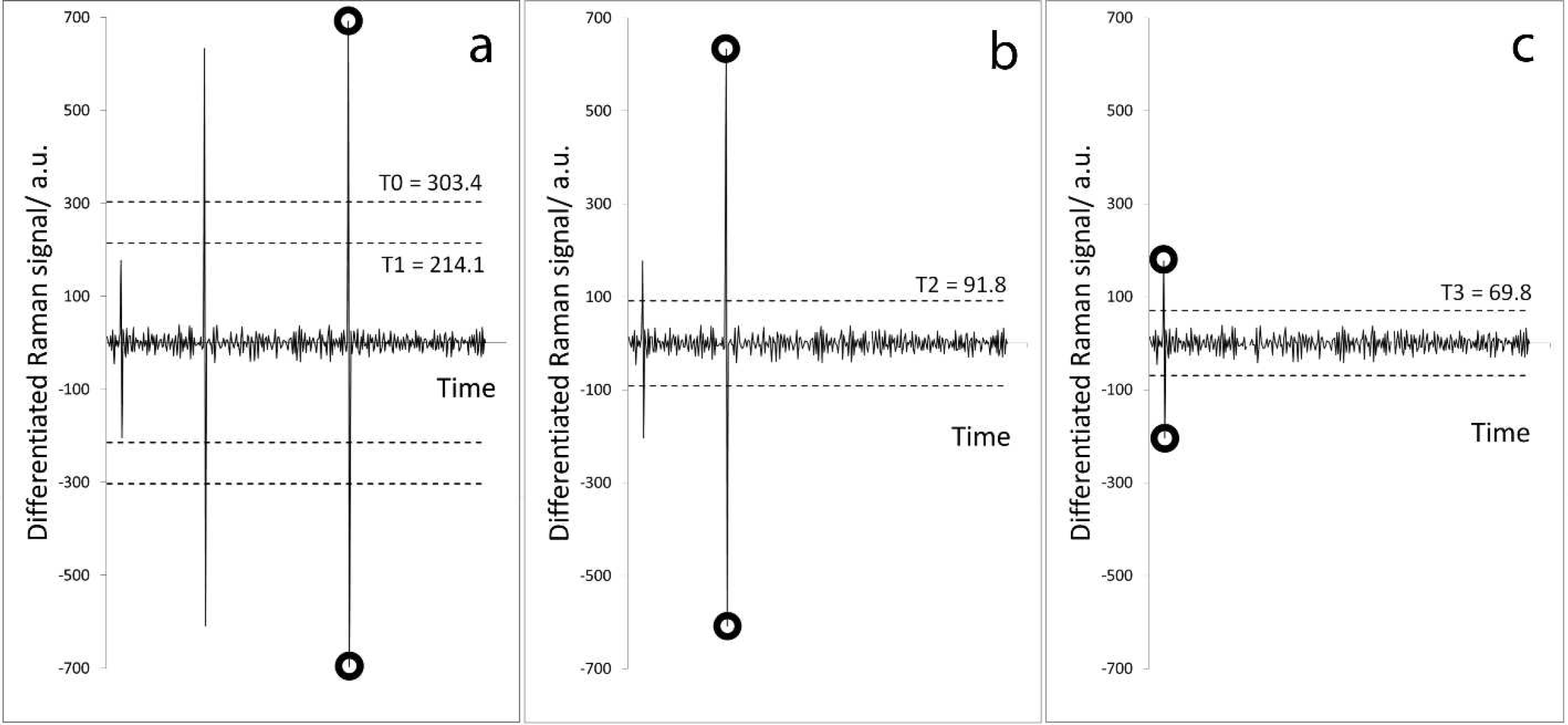
When a true cosmic spike has occurred, the intensity change at a specific wavenumber will change over time as illustrated in the top part of Fig. 3a. The differentiated representation of the data is shown in the lower part of Fig. 3a, demonstrating the characteristic positive and negative features. Before the outliers identified in steps 2 and 3 can be labeled as cosmic spikes two additional tests are implemented to improve accuracy of detection:

The first test removes (from the suspicion list) situations where, for pairs of consecutive points in the differentiated data (D), a negative value point is not immediately preceded by a positive value point, and a positive value point is not immediately followed by a negative value point (Figs. 3b–3e). This test is a mathematical manifestation of the condition that a Raman signal contaminated with a single cosmic spike should return to the expected intensity in the following spectrum.

The pair of points in D (positive followed by negative) that pass the previous test are subject to another test that checks whether the two points adjacent to the outlier pair are also outliers. The goal is to filter out all sequences of repeated rises and repeated falls in intensity S over time (top parts of Figs. 3f–3h) that would imply that a suspected cosmic spike is not a sudden event but rather a consequence of a more prolonged sequence of significant intensity changes that cannot be caused by a single cosmic ray and therefore should be examined more carefully. The present algorithm is designed to detect single cosmic spikes and such complex sequences of signal variation are removed from the suspicion list.

Fig. 1.

An example of original and differentiated data sets for Raman spectra measured over a period of time: (a) original data set; (b) differentiated along the time (sample) axis; (c) differentiated along the wavenumber axis.

Fig. 2.

An illustration of the cosmic spike detection process for real data at a selected wavenumber: during the first stage (a) the maximum and minimum values (shown as black circles) in the differentiated Raman signal are found. If they exceed the threshold (shown with horizontal dotted lines) they are removed from the data set and the process is repeated with the next maximum and minimum values (b) until no more points exceed the threshold (c). In this figure, T0 denotes the threshold obtained using the standard deviation calculated from all data points. T1, T2, and T3 are thresholds obtained by successive removal of maximum and minimum values in the data. All thresholds are calculated as 4σ.

Fig. 3.

Schematic illustration of cosmic spike detection filters for simulated data. The points correspond to intensity measurements at a single wavenumber over time (top part, shown in grey) and the corresponding differentiated data (bottom part, shown in black). The dotted lines show threshold boundaries. Example (a) illustrates the occurrence of a true cosmic spike. Examples (b)-(e) fail test 4a and examples (f)-(h) pass test 4a but fail test 4b.

Extension to Shoulders and Replacement of Contaminated Data Points. The software supplied with the Raman spectrometer used in our experiments has an apodization feature that shapes the intensity profile of the spectra by adding additional data points between the pixels. It results in an increase of bandwidth of a typical cosmic spike to about 30 pixels or 9 cm⁻¹ (Fig. 4a). Cosmic spikes are more difficult to remove from apodized spectra and most existing spike removal algorithms cannot handle them due to increased spike widths. However, apodization is commonly used in the Raman community and the present algorithm was deliberately designed to be compatible with both raw and apodized spectra. The challenge with apodized spectra is that only the intense central area of the spikes are corrected while their less intense shoulders remain undetected and the corrected spectra look distorted as shown in Fig. 4b. The distortions are insignificant as the remaining shoulders are within the threshold limit. However, their removal improves the appearance of the spectra and therefore may be useful to perform.

Fig. 4.

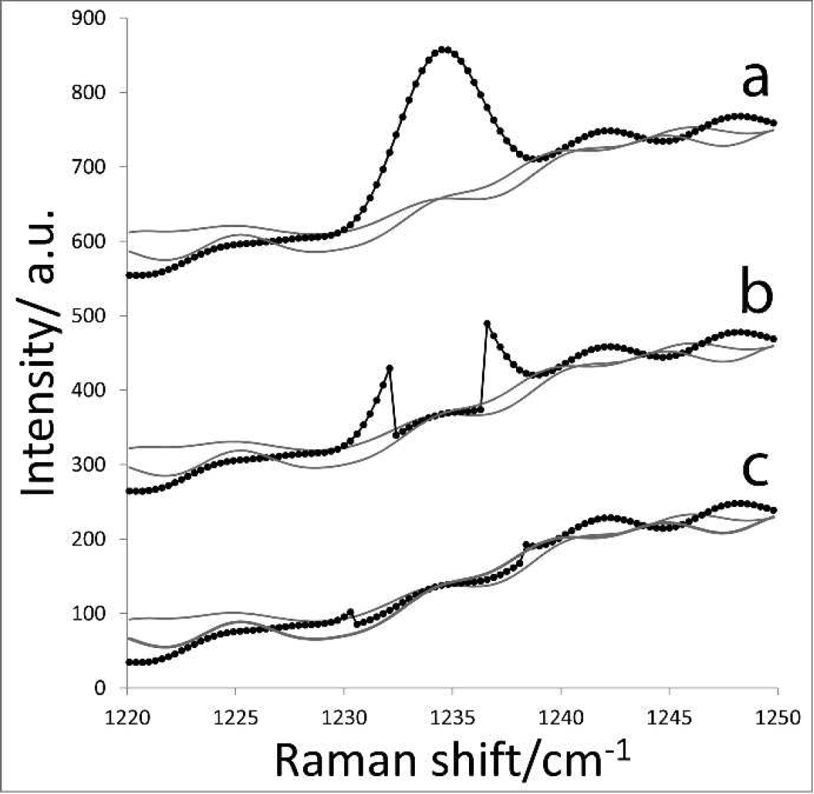
Effect of shoulder extension step on cosmic spike correction. Black line with experimental points shows a spectrum contaminated with a cosmic spike. Gray lines indicate neighboring spectra. (a) Original spectral fragments; (b) corrected spectrum; (c) corrected spectrum followed by automatic extension of spike shoulders.

To extend the detected spike centers to their full widths, the cosmic spike shoulders are located by applying a much lower value of threshold t2_(1,j) (e.g., half of the standard deviation instead of four standard deviations) to the D matrix. Because the standard deviations have already been calculated, the detection is performed in one step in contrast to the iterative procedure described in steps 2 and 3 in the previous section.

Using a very low threshold causes a substantial presence of false positives (spectral noise) in the resulting matrix. Tests 4a and 4b remove some of the noise, but the main mechanism of separating cosmic spike shoulders from noise is based on rejection of all outliers except for those directly adjacent to the detected cosmic spikes (along the wavenumber axis). Any such pixel that exceeds the low threshold value t2 becomes part of that spike and the matrix of cosmic spikes is updated. Such expansion of the spike boundaries is repeated, pixel by pixel, in a conditional loop, until either the threshold t2 for both neighboring pixels is no longer exceeded or the maximum predefined number of iterations is performed, whichever condition is met first. The maximum number of iterations is set to half the width of the typical cosmic spike to prevent irrelevant extension of the spike boundaries beyond the typical spike width that is a known constant for a given Raman instrument (30 pixels in our instrument). Figure 4c shows the effect of spike extension on improving appearance of the spike-corrected spectrum. The remaining discontinuities on Fig. 4c at the spike boundaries are no bigger than the spectral noise and are not visible when more neighboring spectra are overlaid. These discontinuities are too small to influence the information contained in the spectra. For these reasons further smoothing of the spike boundaries in the corrected spectra were not considered. Note that shoulder correction may not be necessary when apodization is not used. This feature was added to the algorithm to demonstrate its ability to work with interpolated spectra and filter cosmic spikes occupying more than one pixel in the detector.

Once all cosmic spikes have been processed in this way the signal at the contaminated pixels can be replaced using a missing-point algorithm. In the present work, we replaced the contaminated data points with the average signal of two adjacent spectra at that wavelength.

EXPERIMENTAL SECTION (VALIDATION)

The algorithm was tested on the five process Raman data sets listed in Table I. All Raman spectra were obtained using an Rxn-1 Raman spectrometer (Kaiser Optical Systems) and 250 mW of 785 nm laser excitation with either an immersion ballprobe¹⁷ (data set 1) or a specially designed probe for microfluidic applications¹⁸ (data sets 2–5). The immersion ballprobe was fitted to an MR Filtered Probe Head (Kaiser Optical Systems). In all cases one excitation and one collection fiber were used for spectral acquisition.

TABLE I.

Summary of the Raman data sets used to validate the cosmic spike filter.

Data set number	Size (samples X pixels^a)	Reaction type	Process type	Contamination level	Smoothness of compositional change in time
1	332 × 11069	Fermentation	Batch	High	Smooth
2	1746 × 5449	Esterification	CF^b/microfluidic	Moderate	Not smooth
3	650 × 6400	Mixing	CF/microfluidic	Low	Not smooth
4	180 × 6399	Knoevenagel	CF/microfluidic	Low	Smooth
5	460 × 6398	Knoevenagel	CF/microfluidic	Low-moderate	Smooth

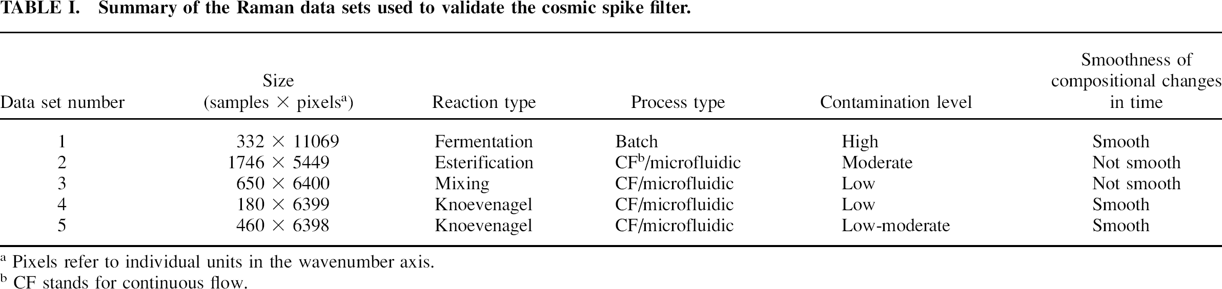
Pixels refer to individual units in the wavenumber axis.

CF stands for continuous flow.

The data sets were selected to study the utility of the cosmic spike filter in a variety of typical process types:

(1)

is a heavily contaminated Raman data set obtained from batch fermentation of glucose. Its variable baseline was used to study the effect of background variations on the filter performance. Data set 1.1 will represent the original data and 1.2 will represent the data after removing the background using the curve-fitting procedure¹⁹ with a 6th-order polynomial baseline rejection method.

(2)

is an acid-catalyzed esterification reaction between methanol and acetic acid carried out in continuous flow. The reaction was studied at four different flow rates that were dynamically changed in a step-wise manner. The steps caused fast compositional changes in the signal collection volume that could potentially lead to misdetection of cosmic spikes. To make these changes more pronounced, data set 2 was modified by selecting 30 consecutive spectra at each flow rate and adding them together as shown in Fig. 5. This represents a realistic situation where a sample is measured at a series of different conditions (or when there are different sets of samples with different compositions) without any intermediate data points. The original data set is denoted as 2.1 and the modified data set as 2.2. The modified data set consists of 210 spectra.

(3)

refers to intermittent pumping of methanol and acetic acid into a microreactor with 5 min intervals (5 min “on” and 5 min “off”). Abrupt resumptions of pumping caused sharp peak-shaped compositional changes in the flow that were detected with Raman spectroscopy. This data set is an example of a process where very fast changes of Raman peak intensities resemble the characteristics of cosmic spikes and thus could be misinterpreted by the algorithm. It usually occurs in continuous flow systems with unstable pumping or other sources of instability.

(4)

is monitoring of a continuous flow Knoevenagel condensation reaction in a steady state. In contrast to data set 3 the chemical composition in the reaction mixture varied in a smooth but random manner due to mixing instabilities. Low contamination of this data set with cosmic spikes is useful to evaluate the ability of the cosmic spike filter to distinguish cosmic spikes from noise and repeated spectral changes.

(5)

is the same Knoevenagel condensation reaction implemented in a “flushed steady-state” methodology²⁰ that assumes fast analysis of a rapidly flowing media with a compositional gradient along the flow path. This gradient mimics situations where chemical composition of the reaction mixture changes continuously and rapidly, causing significant differences between adjacent Raman spectra within the data set.

Fig. 5.

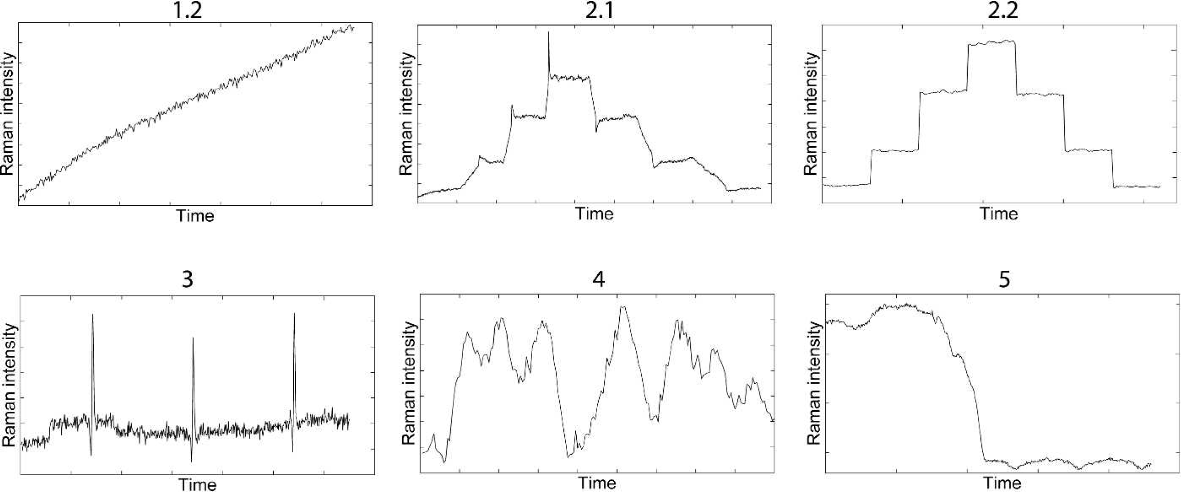
Plots of intensity versus time for the most variable Raman peak in each data set indicating the dynamics of compositional changes (see Table I). The following Raman peaks were used: 879 cm⁻¹ for data set 1.2, 893 cm⁻¹ for data sets 2.1 and 2.2, 1030 cm⁻¹ for data set 3, and 1601 cm⁻¹ for data sets 4 and 5.

The challenges for the cosmic spike filter were to correctly detect cosmic spikes in all of these very diverse data sets and to distinguish the cosmic spikes from the inherent spectral noise and Raman band intensity variations to preserve the valuable chemical information recorded in the Raman spectra. Furthermore, this should be achieved in a completely automated way, without the need to modify or preset any parameters.

To illustrate the importance of all cosmic spike recognition steps with regards to spike detection accuracy, three variants of the original algorithm were created, each being deprived of at least one functional feature related to cosmic spike recognition:

Modified algorithm A: standard deviations σ in steps 2 and 3 are calculated without removing outliers from the data set; tests 4a and 4b are applied.

Modified algorithm B: σ is calculated as described in steps 2 and 3; test 4a is applied; test 4b is not applied.

Modified algorithm C: σ is calculated as described in steps 2 and 3; tests 4a and 4b are both not applied. Any positive point in the D matrix that exceeds the threshold is recognized as a representation of a cosmic spike without further analysis. Negative outliers in the D matrix are ignored.

RESULTS AND DISCUSSION

Selection of Threshold. There is no universal way to detect cosmic spikes with absolute certainty. Although intense cosmic spikes can be easily identified as outliers visually, spikes with lower intensities can be difficult to distinguish from spectral noise or intensity variations of Raman bands. Accuracy of cosmic spike detection depends on the spike intensity, random spectral noise and systematic variations of the spectral background and Raman bands. Variable background can be subtracted from the spectra and intensity variations of Raman bands are assumed to be smooth during process monitoring. Therefore the interplay between random spectral noise and spike intensity remains the only factor that cannot be readily controlled; it determines the accuracy of cosmic spike detection in the same way as reproducibility of an analytical signal determines the limit of detection in chemical analysis. The key parameter to identifying cosmic spikes is the value of the statistical intensity threshold t of the differentiated Raman signal. Its optimal value must be sufficiently high to minimize misdetections and sufficiently low to ensure that all cosmic spikes are detected.

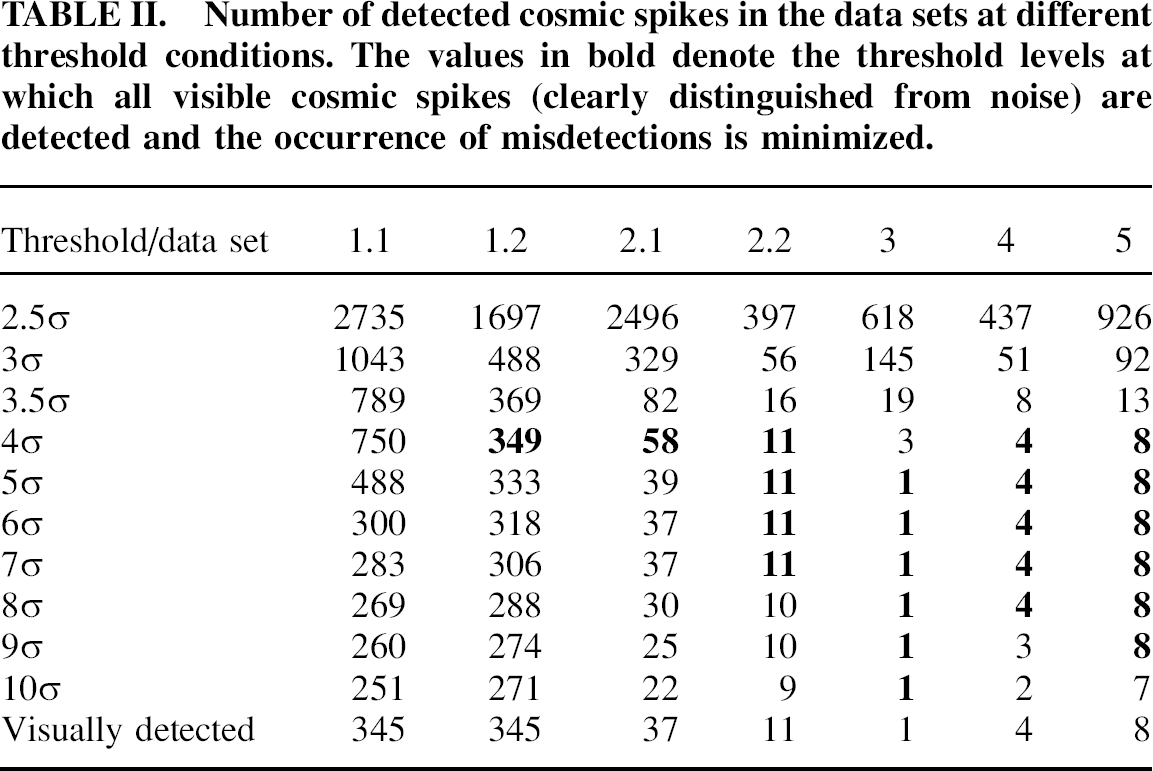
Table II shows the effect of threshold factor on the number of spikes found by the algorithm in the tested data sets. According to the table, all tested data sets require a minimum threshold of 4σ in order to minimize misdetections, while the upper threshold limit varies between the data sets. For data sets 1.2 and 2.1, which contain a large number of cosmic spikes, a threshold value of 4σ is most optimal. For the data sets with low spike abundance (2.2, 3, 4, and 5), the range of optimal thresholds extends up to 10σ, typically starting from 4σ or 5σ.

TABLE II.

Number of detected cosmic spikes in the data sets at different threshold conditions. The values in bold denote the threshold levels at which all visible cosmic spikes (clearly distinguished from noise) are detected and the occurrence of misdetections is minimized.

Threshold/data set	1.1	1.2	2.1	2.2	3	4	5
2.5σ	2735	1697	2496	397	618	437	926
3σ	1043	488	329	56	145	51	92
3.5σ	789	369	82	16	19	8	13
4σ	750	349	58	11	3	4	8
5σ	488	333	39	11	1	4	8
6σ	300	318	37	11	1	4	8
7σ	283	306	37	11	1	4	8
8σ	269	288	30	10	1	4	8
9σ	260	274	25	10	1	3	8
10σ	251	271	22	9	1	2	7
Visually detected	345	345	37	11	1	4	8

TABLE III.

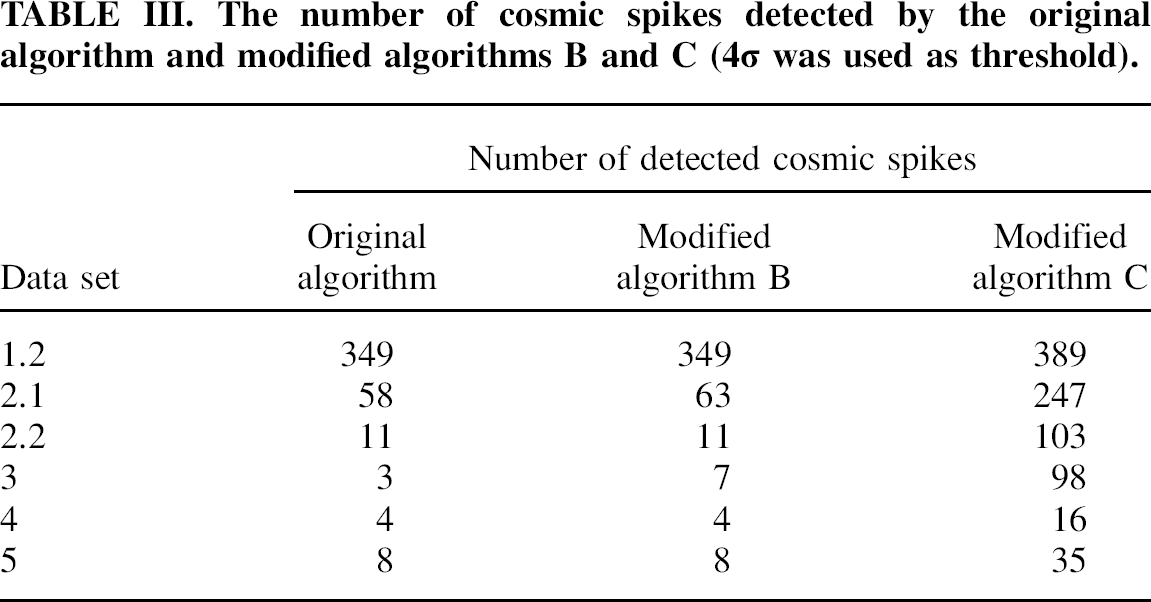
The number of cosmic spikes detected by the original algorithm and modified algorithms B and C (4c was used as threshold).

	Number of detected cosmic spikes
Data set	Original algorithm	Modified algorithm B	Modified algorithm C
1.2	349	349	389
2.1	58	63	247
2.2	11	11	103
3	3	7	98
4	4	4	16
5	8	8	35

Note that in data set 2.1 a threshold value of 5σ seems to be more optimal than 4σ due to an apparently smaller number of misdetections (39 is closer to 37 than 58). However, the table does not show that clearly visible cosmic spikes were missed at 5σ in this data set. By reducing the threshold to 4σ the missed spikes were detected although at the expense of adding more misdetections to the results.

Given that mistaking spectral noise for cosmic spikes does not cause any significant damage to the information content and that some misdetections of this type are statistically expected in all data sets, it is reasonable to ease the requirements for threshold selection and consider the possibility to find a common optimal threshold for all tested data sets. The data in Table II suggest that 4σ can be used as the common optimal threshold; it ensures detection of all visually noticeable cosmic spikes and only a low chance of misdetecting spectral noise for cosmic spikes.

It is important to note that Table II is generated with fairly large steps between threshold values. Additional values between existing points (such as 4.2σ, 4.5σ) could have been added and the result discussed in more detail. However, the present level of detail is consistent with some uncertainty in judging the origin of spikes when their intensities are comparable with spectral noise and the low importance of completely avoiding misdetections. By suggesting an optimal fixed threshold value of 4σ without comparing it with other values in the range 3.5σ−5σ we acknowledge that (1) the best threshold may be slightly different depending on the data set and, importantly, (2) that there is little or no benefit to optimize it to higher precision than has been demonstrated here. Assuming that all variations in the data set are normally distributed (which is a very approximate model when expecting possible baseline correction artifacts and chemistry-induced intensity variations), 4σ corresponds to a reasonable boundary that represents (a) humans' ability to visually see an outlying spike, (b) a fairly low statistical expectation of outliers (spectral noise) above this boundary, and (c) a window within which cosmic spikes have a negligible potential to notably distort the data.

The ability of the present algorithm to perform effectively with a wide range of data types without changing the threshold is unmatched by other cosmic correction methods. This can be explained by the use of a derivative prior to calculating the signal variation and performing these calculations independently for each wavenumber.

It is also worth noting that baseline variations in data set 1.1 have a significant effect on the algorithm's fidelity. Table II reveals a large number of misdetections that occurred by applying the algorithm to data set 1.1 with thresholds 4σ and 5σ. Finding a more acceptable threshold may not always be possible for such data sets, especially when the baseline fluctuates in a random or unpredicted manner. Therefore, it is necessary to perform a correction of the variable baseline before using the cosmic spike filter.

Effect of Calculating Standard Deviations Without Removing Outliers. Applying modified algorithm A to data set 2.1 revealed its compromised ability to detect cosmic spikes of lower intensity when more than one spike occurs at the same wavenumber. This effect is demonstrated in Fig. 2, which is based on data set 1.2. The figure shows differentiated Raman signal versus time for a detector pixel where three cosmic spikes occurred throughout the experiment. The threshold obtained without removing outliers (T0) is too high to detect one of the spikes. Even after removing the first pair of outliers (shown as circles in Fig. 2a) the threshold is still too high (T1). Although using a lower threshold factor (e.g., 3σ instead of 4σ) can help detect some cosmic spikes, it also causes a significantly higher chance of misdetections at other pixels that contain one or no cosmic spikes.

Application of modified algorithm A to the other data sets produced similar or identical results to those obtained with the original algorithm, which can be explained by the low level of contamination in these data sets, i.e., the absence of any wavenumber affected by more than one cosmic spike.

These results demonstrate that excluding outliers from standard deviation calculations is essential for the filter to correctly detect multiple cosmic spikes on one wavenumber and to ensure independence of the result from other significant outliers regardless of their origin.

Effect of Filtering Non-Cosmic Spikes Using Tests 4a and 4b. Although we assumed that gradual compositional changes during a chemical process make intensity variations in Raman spectra smooth, there are several exceptions that can result in misdetection and need to be accounted for.

These exceptions include significant but repeated signal changes, as well as step increases or decreases in intensity caused by compositional changes in the signal collection volume. In continuous-flow processes, these variations occur due to mixing/pumping instability (data sets 3 and 4), step-wise modifications of flow rate (data sets 2.1 and 2.2), and changes in temperature or other conditions (data sets 1 and 5). In batch reactions, fast variations of spectral response can be caused by thermal effects, dilution, or addition of reagents to the reaction mixture during the process. The algorithm's ability to distinguish cosmic spikes from the effects of such variations on Raman spectra is necessary to prevent loss of important process information while using the cosmic spike filter.

The present algorithm is designed to retain the pertinent chemistry-related information in Raman spectra while removing the cosmic spikes by performing four independent tests for each suspected spike. Firstly, a strong rise in the Raman intensity is detected. Secondly, it is confirmed that the signal returns to the expected value in the following spectrum. In the third and fourth tests, spectra recorded before and after the suspected spectrum are assessed to identify repeated increases and decreases in intensity at the selected wavenumber. This multi-step approach allows cosmic spikes to be effectively distinguished from process/chemical variations, as illustrated by the results in Table I II where the effects of applying the original and modified algorithms to the tested data sets are compared.

Comparison of the number of spikes found by the original algorithm and algorithm C provides information about the aggregate importance of tests 4a and 4b. The difference in the results between algorithms B and C indicates the contribution of test 4a. And finally, algorithm B in comparison with the original algorithm shows the importance of test 4b.

The significantly higher number of misdetections obtained with algorithm C compared to those of algorithm B highlights the importance of test 4a in distinguishing cosmic spikes of lower intensity from random spectral noise.

The role of test 4b is revealed by comparing the results obtained with the original algorithm and algorithm B. These results are different only with data sets 2.1 and 3, which contain abrupt peak-shaped changes in Raman band intensities that can be easily confused with cosmic spikes. Therefore, test 4b is not important in data sets with smooth variations in the sample composition. However, it greatly reduces the risk of mistaking abrupt intensity variations for cosmic spikes, which is very useful in continuous flow systems with high pumping instability.

Influence of the Data Set Size. As the present algorithm is based on statistical analysis of variation at each wavelength, its performance should depend on the data set size (number of samples).

To study this effect, 13 data sets with different numbers of samples were generated by selecting the first n spectra from data set 1.2, where n changed incrementally from 5 to 200. The original algorithm was applied to each of these sub-sets and the number of detected spikes was compared with the number of cosmic spikes found by the reference method. The reference method involved applying the original algorithm to the full data set 1.2 and determining how many detected cosmic spikes were found in the corresponding first n spectra. Ideally, these numbers should be the same or similar. However, the results show that this is not always the case. According to Fig. 6, as the number of samples is reduced to 40 or lower the algorithm generates an increasingly higher number of misdetections. This observation suggests that the algorithm is universally applicable to Raman data sets with no less than 40 to 50 spectra. For smaller data sets, the threshold value has to be increased.

Fig. 6.

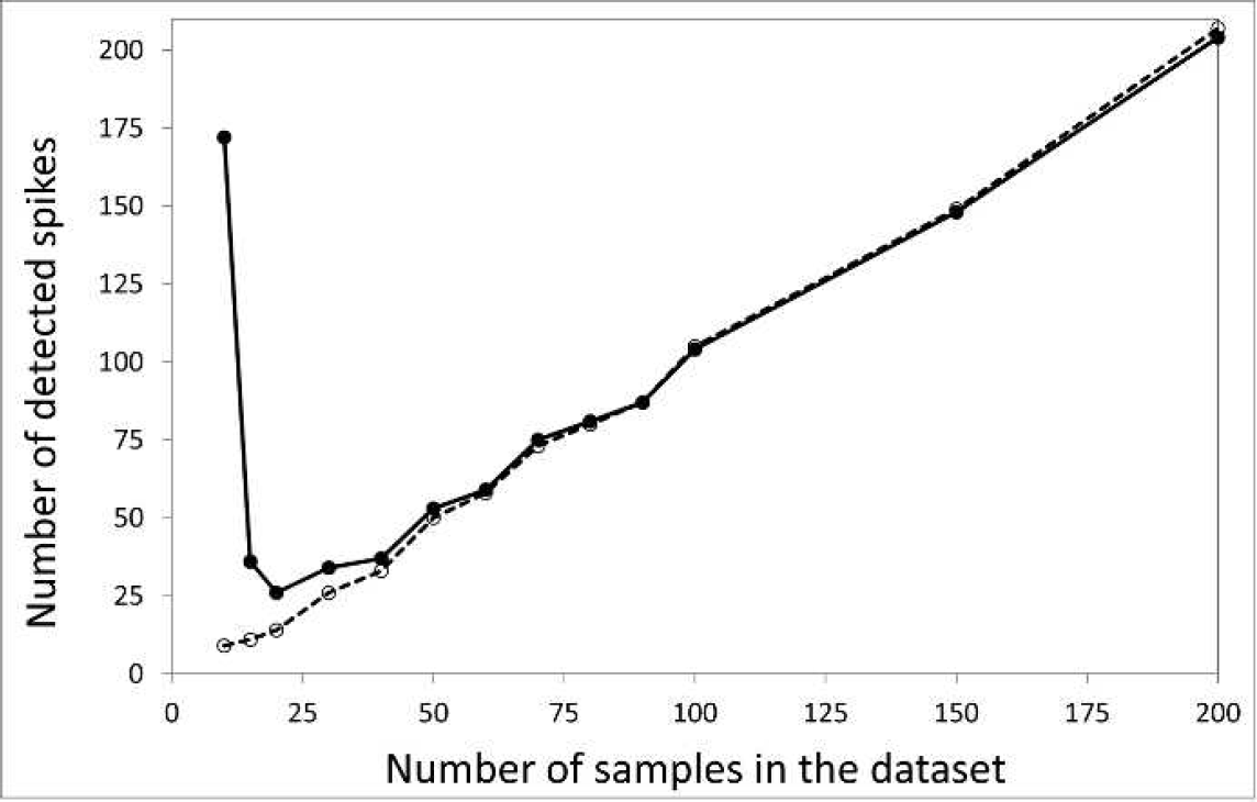
Effect of data set size on the algorithm accuracy. The solid line shows the number of detected spikes in individual sub-sets and the dashed line represents the number of cosmic spikes found from the full data set.

Limitations for Operation in Real Time. The presented algorithm is suitable for post-experiment data processing. With a few limitations it can also be used for automatic spike removal in real time. Because the present algorithm requires 40 to 50 spectra to build a reliable matrix of variances at each wavenumber channel it will have to rely on a historical spectral database in the beginning of the process or be started after the initial 40 to 50 spectra are collected. This would not be a significant problem because most process Raman data is collected in the sub-minute time frame. The second limitation is a delay in response due to the requirement of acquiring two additional spectra to achieve the most accurate identification of cosmic spikes. The effect of this delay can be reduced by either increasing the frequency of measurements or by giving preliminary estimates in real time based only on the data acquired prior to the spectrum under analysis.

CONCLUSIONS

A novel fully automated algorithm for detecting cosmic spikes in process Raman data sets has been developed and validated using a wide range of experimental data. A unique multi-stage spike recognition process has been shown to provide exceptional efficiency in distinguishing low-intensity cosmic spikes from random spectral noise and variations of Raman peaks. The algorithm operates reliably without any user-defined parameters for data sets containing more than 40 to 50 spectra. Given the wide range of data types used to test the algorithm, it has the potential to be applicable to any process Raman data set without modifications, even if it contains step-change variations in the intensities of Raman peaks. It takes less than 3 seconds for an ordinary computer to process a million data points, offering the possibility of fast automatic removal of cosmic spikes in real time. Although the real-time detection will have to be delayed by one or two spectra that are necessary for the correct identification of cosmic spikes, the effect of this delay can be reduced by increasing measurement frequency.

Footnotes

ACKNOWLEDGMENTS

SM was supported by the Scottish Funding Council, Centre for Process Analytics and Control Technology (CPACT), Center for Process Analysis and Control (CPAC), the University of Strathclyde, Mac Robertson fund, and Royal Society of Chemistry. The Royal Society is thanked for the award of a University Research Fellowship to AN. The authors are grateful to Wes Thompson and Shannon Ewanick for acquiring the fermentation data, and Tom Dearing, for useful comments during preparation of the manuscript.

References

Denson

S.C.

Pommier

C.J.S.

Denton

M.B.

“The impact of array detectors on Raman spectroscopy”. J. Chem. Educ. 2007. 84(1): 67–74.

Phillips

G.R.

Harris

J.M.

“Polynomial Filters for Data Sets with Outlying or Missing Observations: Application to Charge-Coupled-Device-Detected Raman Spectra Contaminated by Cosmic Rays”. Anal. Chem. 1990. 62(21): 2351–2357.

Hill

Rogalla

“Spike-Correction of Weak Signals from Charge-Coupled-Devices and its Application to Raman-Spectroscopy”. Anal. Chem. 1992. 64(21): 2575–2579.

Takeuchi

Hashimoto

Harada

“Simple And Efficient Method To Eliminate Spike Noise From Spectra Recorded On Charge-Coupled Device Detectors”. Appl. Spectrosc. 1993. 47(1): 129–131.

Zhang

D.M.

Jallad

K.N.

Ben-Amotz

“Stripping of cosmic spike spectral artifacts using a new upper-bound spectrum algorithm”. Appl. Spectrosc. 2001. 55(11): 1523–1531.

Zhao

“Image curvature correction and cosmic removal for high-throughput dispersive Raman spectroscopy”. Appl. Spectrosc. 2003. 57(11): 1368–1375.

Zhang

Henson

M.J.

“A practical algorithm to remove cosmic spikes in Raman imaging data for pharmaceutical applications”. Appl. Spectrosc. 2007. 61(9): 1015–1020.

Cappel

U.B.

Bell

I.M.

Pickard

L.K.

“Removing Cosmic Ray Features from Raman Map Data by a Refined Nearest Neighbor Comparison Method as a Precursor for Chemometric Analysis”. Appl. Spectrosc. 2010. 64(2): 195–200.

Chew

“Information-theoretic chemometric analyses of Raman data for chemical reaction studies”. J. Raman Spectrosc. 2011. 42(1): 36–47.

10.

Dai

“An Improved Algorithm to Remove Cosmic Spikes in Raman Spectra for Online Monitoring”. Appl. Spectrosc. 2011. 65(11): 1300–1306.

11.

Zhang

Hanna

J.D.

Ben-Amotz

“Single scan cosmic spike removal using the upper bound spectrum method”. Appl. Spectrosc. 2003. 57(10): 1303–1305.

12.

Katsumoto

Ozaki

“Practical algorithm for reducing convex spike noises on a spectrum”. Appl. Spectrosc. 2003. 57(3): 317–322.

13.

Soneira

M.J.

Perez-Pueyo

Ruiz-Moreno

“Raman spectra enhancement with a fuzzy logic approach”. J. Raman Spectrosc. 2002. 33(8): 599–603.

14.

Behrend

C.J.

Tarnowski

C.P.

Morris

M.D.

“Identification of outliers in hyperspectral Raman image data by nearest neighbor comparison”. Appl. Spectrosc. 2002. 56(11): 1458–1461.

15.

Miljkovic

Chernenko

Romeo

M.J.

Bird

Matthaus

Diem

“Label-free imaging ofhuman cells: algorithms for image reconstruction of Raman hyperspectral datasets”. Analyst. 2010. 135(8): 2002–2013.

16.

Zhang

D.M.

Ben-Amotz

“Removal of cosmic spikes from hyperspectral images using a hybrid upper-bound spectrum method”. Appl. Spectrosc. 2002. 56(1): 91–98.

17.

Marquardt

B.J.

Burgess

L.W.

“Optical immersion probe incorporating a spherical lens”. US Patent 06977729. Filed 2001. Issued 2005.

18.

Mozharov

Nordon

Girkin

J.M.

Littlejohn

“Non-invasive analysis in micro-reactors using Raman spectrometry with a specially designed probe”. Lab Chip. 2010. 10(16): 2101–2107.

19.

Lieber

C.A.

Mahadevan-Jansen

“Automated method for subtraction of fluorescence from biological Raman spectra”. Appl. Spectrosc. 2003. 57(11): 1363–1367.

20.

Mozharov

Nordon

Littlejohn

Wiles

Watts

Dallin

Girkin

J.M.

“Improved Method for Kinetic Studies in Microreactors Using Flow Manipulation and Noninvasive Raman Spectrometry”. J. Am. Chem. Soc. 2011. 133(10): 3601–3608.