Continuous Online Fourier Transform Infrared (FT-IR) Spectrometry Analysis of Hydrogen Chloride (HCl),Carbon Dioxide (CO 2 ),and Water (H 2 O) in Nitrogen-Rich and Ethylene-Rich Streams

INTRODUCTION

Mid-infrared (IR) optical spectroscopy is an information-rich process analysis option that is applicable to a large variety of chemical species present in the chemical and petrochemical industries. For gas-phase streams, such as those with a balance of nitrogen or ethylene, Fourier transform IR (FT-IR) is useful for capturing both quantitative and qualitative process information with minimal chemometric modeling due to the narrow peak widths of most gas-phase transitions. Gas-phase FT-IR had its start as a continuous process analysis technique for chemical and petrochemical industries in the 1980s ¹ and has since continued to gather momentum toward acceptance as a robust and reliable process analysis methodology. ² The variety of potential applications and installation configurations continues to grow as hardware and software capabilities continue to develop and computing speeds increase. ³

Spectroscopy has been used not only to monitor various compounds, it has also provided information to control a process. For example, FT near-IR (FT-NIR) spectroscopy was used to monitor the spectra of monoalkylated alkenes and to guide process control.^4–6 Special considerations must be taken when the compounds monitored are of a corrosive nature.^7,8 An FT-IR spectrophotometer equipped with an 8 m gas cell having solid nickel mirrors was used to determine the amount of water (H₂O) in anhydrous hydrogen chloride (HCl) samples as well as impurities in gaseous chlorine. ⁸

The ability to monitor process compositions in real time has proven valuable for both temporary and permanent spectrometer installations. Production plants frequently only “know” what is present in their process by models or infrequently grab samples that do not capture the actual composition or variation occurring; and sometimes, this lack of full-process understanding leads to process operation upsets that result in downtime or producing off-grade product. In such cases, temporary FT-IR spectrometers have proven to be the key to providing the process understanding required to determine and address the root cause of the operation difficulties. ⁹

On occasions such as in the application discussed here—online analysis of HCl, carbon dioxide (CO₂), and H₂O in nitrogen and ethylene streams—the measurement starts as a temporary troubleshooting method and then becomes a permanent online analysis system when high value is captured from information generated by the system.

The previous analytical methodology for these streams was a periodic gas detector tube (e.g., Dräger-Tube® [Dräger Safety Canada Ltd.] or GASTEC® Tube [GASTEC, Japan]). This technology works by pulling a sample through a small glass tube containing packing with an indicator that changes color in the presence of the analyte of interest and, unfortunately, some other interfering components. Although cheap, analysis by a gas detector tube is time-consuming, not highly reproducible, and cannot be used to capture continuous data. Also, a single gas detection tube cannot be used to monitor multiple components.

In this work, the goal was to provide online measurements of HCl, CO₂, and H₂O in two gas streams, with one stream being primarily nitrogen and the other being ethylene-rich. Measuring impurities in nearly pure ethylene by mid-IR spectroscopy is difficult, because of ethylene's strong absorbance in this region. This measurement is complicated further by the presence of other light hydrocarbons (e.g., ethane, methane, propylene) at low levels (<1%). HCl is a specific challenge because it is overwhelmed by very strong ethylene absorbance. This work describes the developments that led to obtaining a robust HCl measurement, as well as CO₂ and H₂Oinan ethylene-rich environment.

EXPERIMENTAL

The long-path FT-IR system used here is versatile for low-concentration, gas-phase in situ monitoring due to its high resolution, long pathlength, ease of method development, and simple quantitative model-building integration within the vendor's software. In general, any mid-IR spectrometer having a resolution of better than 4 cm⁻¹ and a pathlength of approximately 3–6 m could be used for the analysis with the proper control and modeling software. In this particular scenario, the spectrometer used was an MKS MultiGas™ 2032 with a 5.11m Herriott type multipass cell using the MG2000 software program version 06.31 supplied with the analyzer. An extensive library of more than 200 species of gas-phase spectra that can be used directly as reference spectra for model building is also available with the MKS system. HCl, CO₂, and H₂O spectra from this library were used in the initial model building for online analysis in ethylene.

ANALYTICAL METHOD

The FT-IR used a spectral resolution of 1 cm⁻¹ in the range from 1800 to 5000 cm⁻¹ using the autoreference deresolve 8× capability of the MKS MultiGas 2032 system. The detector cutoff, 5.4 μm (1800 cm⁻¹), was the limiting factor at the low end of the spectral range. The sample cell was temperature controlled, in this case to 60 °C, although ranges from just above ambient to over 100 °C would be acceptable depending on the expected dew point of the analyzed stream. The sample cell pressure in the cell was maintained between 0.8 and 1.2 atmospheres absolute with pressure correction that enabled to account for concentration changes based on the ideal gas law.

The MKS autoreference deresolve 8× algorithm uses the current spectrum deresolved by a factor of 8 as the reference spectrum and therefore eliminates baseline drifts and contributions from broad spectral absorbers, since only transitions narrower than 8 cm⁻¹ full width half-maximum are in the resulting spectrum. The spectral resolution used in this study is 1 cm⁻¹ compared with the 8 cm⁻¹ spectrum as the baseline. The spectrometer has capability down to 0.5 cm⁻¹ in “normal” absorption mode. Elimination of background drifts and broad absorbers increases the long-term stability of the measurement for around-the-clock, continuous operation and removes the need to purge the cell with nitrogen gas (N₂) on a regular basis to obtain a new background spectrum. As HCl, CO₂, and H₂O all have narrow peak widths in the gas phase, this method is suitable in our application. In addition, since the background gas in the application at hand ranges from approximately 5 to > 95 vol% ethylene, the use of the autoreference algorithm should help eliminate effects of broad absorption features in the attempt to quantify the species of interest.

The quantitative FT-IR method used in this case is a modified classical least squares (CLS) model ¹⁰ for each of the components of interest, HCl, H₂O, and CO₂, created within the MG2000 software. A model for ethylene was not created since it was not an analyte of interest, and reference spectra were not readily available from the vendor's spectral library.

In the application discussed here, precision of the analysis is more important than accuracy as one of the major drivers is process trends and direction of change rather than product quality or purity for product release. Development of the model was a two-step process in which the method was initially developed using supplied reference spectra and validated using laboratory samples with N₂ as the balance gas. The second step was re-evaluation of the model based on spectra of the process streams containing approximately 5–95 vol% ethylene to eliminate ethylene interferences in the method. Mid-IR absorption spectra for the analytes of interest in the concentration range of 286–500 ppm are shown in Fig. 1 compared with a spectrum of the background gas (ethylene) at 100 vol%. The spectra in Fig. 1 are regular absorption spectra before the autoreference algorithm. The y-axis in Fig. 1 has all spectra on a common absorbance scale, with many of the ethylene peaks absorbing nearly all of the available light in a few regions (e.g., 2900–3300 cm⁻¹). These spectra are from the reference library provided with the MKS 2032 FT-IR product line. Although the interference from ethylene is significant, there are still regions where each of the analyte species has transitions that can be distinguished from those of ethylene. If an analysis of percent level ethylene were of interest, the transitions at 2569 and 3504 cm⁻¹ (as seen in Fig. 1) would be good candidates for development of a model and can be used as a simple check to verify from which process stream a given spectrum originated.

OPEN IN VIEWER

Fig. 1.

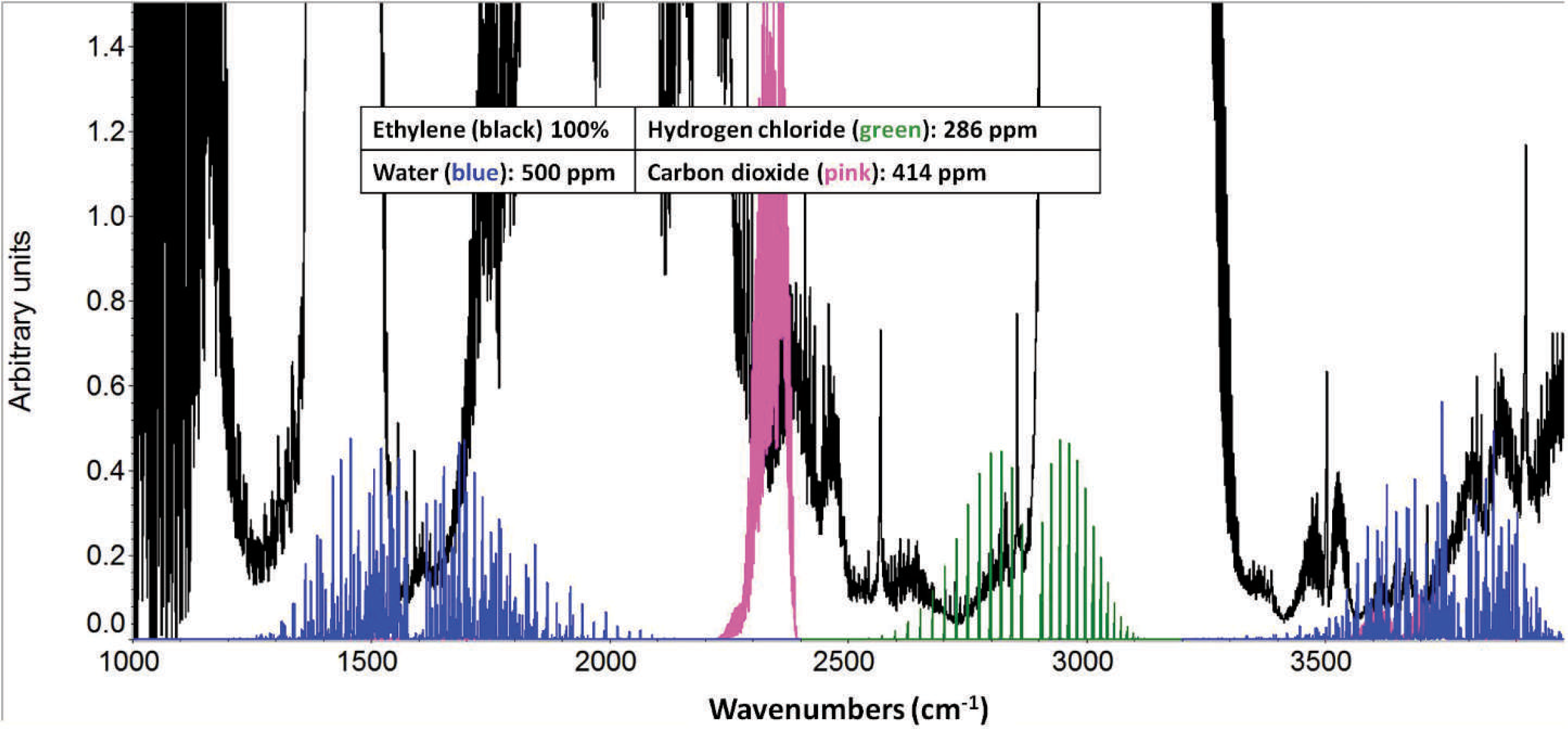
Initial spectral absorption feasibility survey of the critical stream components. Concentrations of the analytes are listed in the legend on the figure.

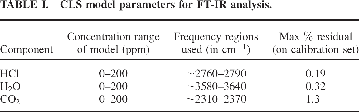
The first step of method development included testing of preliminary models against validation samples of known concentrations of analyte samples in a nitrogen balance. Models were constructed based off of the autoreferenced spectra, not the normal absorbance spectra. In selecting analysis regions for the preliminary models, broad ranges were used in the 2350, 2800, and approximately 3300 cm⁻¹ regions for CO₂, HCl, and H₂O, respectively. Regions of known interference between species were excluded from the analysis along with the estimated regions of ethylene interference based off of the reference spectra shown in Fig. 1. However, without spectra of the actual process background gas, it was impossible to fine tune the models, which were modified classical least squares (CLS) chemometric models based on specified spectral regions with known concentrations of the calibration spectra. All methods/models were built using the MKS MG2000 Calibration Editor program. The spectral regions and concentration ranges for each model—one for each analyte—are provided in Table I. The “maximum percent residual for calibration” column included in Table I is the percent difference between known samples and the corresponding model predictions from the classical least squares method used in the calibration and, therefore, is a measure of the goodness of fit.

OPEN IN VIEWER

TABLE I.

CLS model parameters for FT-IR analysis.

Component	Concentration range of model (ppm)	Frequency regions used (in cm−1)	Max % residual (on calibration set)
HCl	0–200	∼2760–2790	0.19
H2O	0–200	∼3580–3640	0.32
CO2	0–200	∼2310–2370	1.3

The CO₂ prediction model was validated using a single reference cylinder certified as containing 4.76 ppm (±2% relative error). For CO₂, there was a 0.6 ppm offset of the model when applied to plant nitrogen due primarily to plant nitrogen impurities. After adjusting the offset, agreement to the certified cylinder concentrations was within 0.3 ppm absolute, or 6% relative error, over several days.

The preliminary HCl model was validated against a Kin-Tek Trace Source™ (Kin-Tek, TX) permeation tube gas generator with a dry nitrogen carrier gas flow. Concentrations ranging from 1.5 to 15 ppm were used for the validation. The accuracy was determined to be below ±1 ppm absolute or better than 7% relative error.

The H₂O model also was validated against a Kin-Tek Trace Source permeation tube moisture generator but additionally coupled to a National Institute of Standards and Technology (NIST) traceable chilled mirror dew point monitor in the range of 3–28 ppm. There was a +1.3 ppm H₂O offset due to moisture in the laboratory nitrogen purge gas flowing through the detector chamber and interferometer of the FT-IR. However, concentrations compared favorably between the MKS 2032 method and the chilled mirror dew point monitor, resulting in relative errors of <4% and absolute errors <0.4 ppm.

For the ranges considered in this work, the FT-IR methods for the analytes in nitrogen background gas provided good quantification with accuracies of less than ±1 ppm absolute for each component. For the purposes of trending, the process concentrations accuracies of ±5 ppm absolute or 15% relative, whichever is larger, are sufficient. Precision is more important than accuracy. Precision, as calculated by the peak-to-peak (ptp) concentration variation over the course of 5 min under steady-state conditions, was less than ±0.05 ppm (absolute) except in the case of H₂O, for which precision was ±0.1 ppm. The discussion of precision is revisited in the context of steady-state process data. The spectral regions and concentration ranges for the model for each analyte are provided in Table I.

It is clear from an overlap of the ethylene spectrum with those of the analytes of interest (Fig. 1) that models validated in a nitrogen background may not be optimal for use in the process gas. The second step in the model building and validation involved modification of the FT-IR model based on actual process spectra containing 5 to 95 vol% ethylene. It was not possible due to safety and cost constraints to obtain or produce standards of CO₂, HCl, and H₂O in an ethylene background gas for validation. One of the streams, the “nitrogen-rich stream,” contained approximately 5 vol% ethylene, whereas the other stream contained in excess of 95 vol% ethylene. Figure 2A presents the autoreferenced FT-IR spectrum (absorbance) versus wavenumber of a process spectrum of the nitrogen-rich stream overlaid with autoreferenced reference spectra of HCl, CO₂, and H₂O at 100 ppm each. Ethylene is present in large amounts (approximately 5 wt%) compared with the other compounds that are only present at the parts per million level. The nitrogen-rich stream does contain both HCl and H₂O. Note that the peak shapes for the spectra in Figs. 2A and 2B resemble a second derivative lineshape due to the 8× deconvolution autoreferencing algorithm discussed above. Therefore, areas in Fig. 1 where the ethylene absorbance is off the scale show up as intense fluctuations around the baseline in Figs. 2A and 2B (e.g., from 2850 to 3300 cm⁻¹). In Fig. 2A, one can observe that the H₂O and the CO₂ transitions, as well as the HCl P-branch lines above P(3), are clear of ethylene interference. In the ethylenerich stream (Fig. 2B) containing >95 vol% ethylene, as well as potentially low levels of other light hydrocarbons, the ethylene interferes with HCl, H₂O, and CO₂ to a much larger degree. There are also a few obvious ethylene bands in the ethylene rich-stream that could give an indication of a percentage trend of ethylene, namely, transitions at 2569 and 3504 cm⁻¹. It was observed, however, that because ethylene is such a strong absorber over larger portions of the spectrum, the centerburst intensity of the interferogram suited our purposes of stream identification checking while doubling as a useful diagnostic of spectrometer health during continuous operation.

OPEN IN VIEWER

Fig. 2.

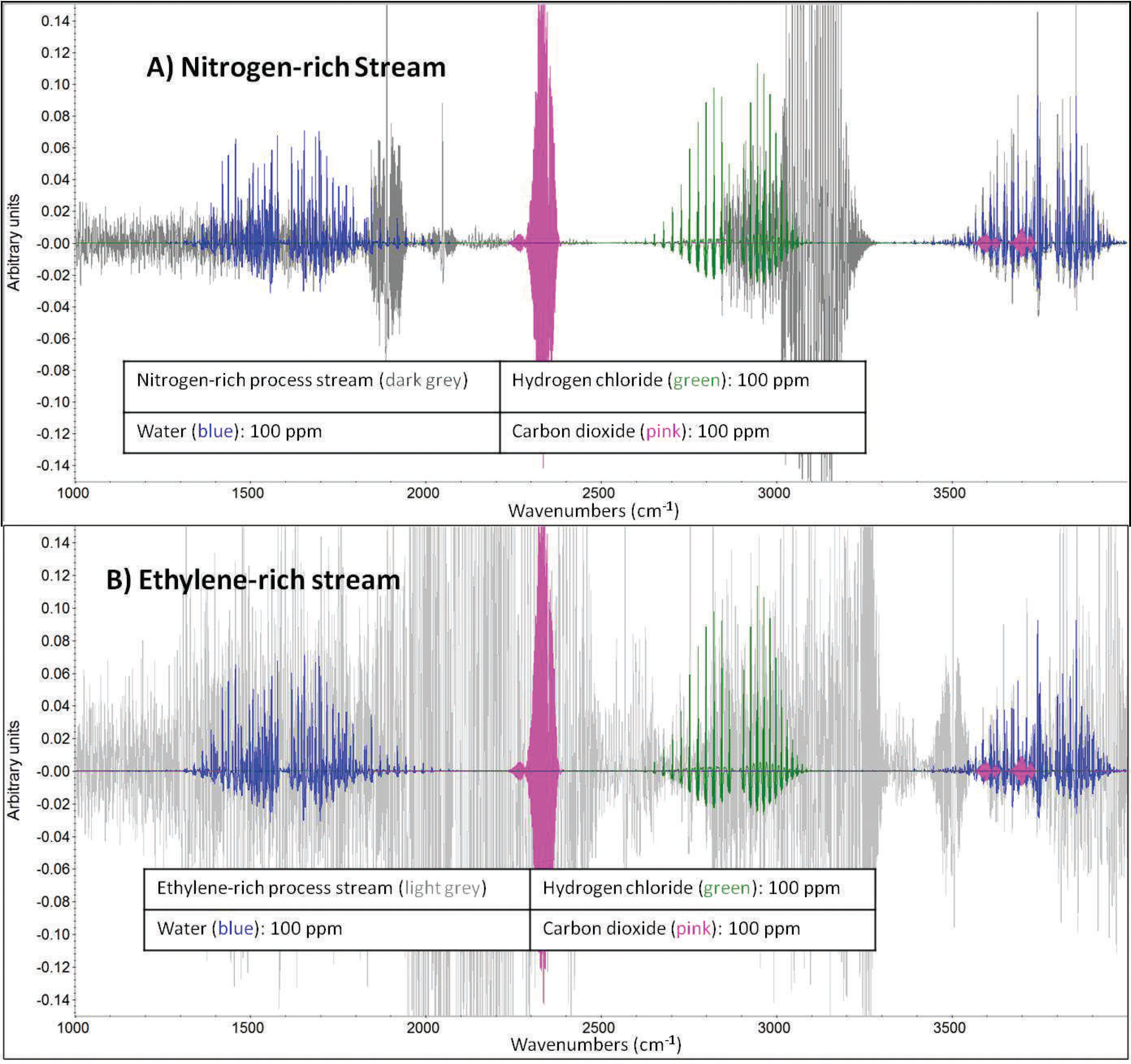
Auto-referenced spectra (absorbance vs. wavelength) of (A) the nitrogen-rich process stream with (B) the ethylene-rich process stream with the three analyte reference spectra at 100 ppm in nitrogen.

One could attempt to look at signal-to-noise ratio (S/N) ratios for the two different streams, but it is difficult to find regions of the ethylene-rich process stream that are suitable for the determination of a baseline noise calculation. The best option is the region from 3410 to 3440 cm⁻¹. In this region, the root mean square error is 0.0034 and 0.0004 arbitrary units for the ethylene-rich and nitrogen-rich streams, respectively. The increased baseline noise of the ethylene stream is expected due to the significantly lower interferogram centerburst intensity (IgramPP) for the stream. The IgramPP for the ethylene-rich stream ranged from 1 to 1.5 V, whereas the IgramPP for the nitrogen-rich stream ranged from 4 to 6 V.

In the ethylene-rich stream, the overlap of the ethylene spectrum with HCl is, as expected, more dramatic than in the nitrogen-rich stream (Figs. 2A and 2B), and in both cases, it is more extreme than was anticipated when generating the initial CO₂ and HCl CLS model. One could develop a separate CLS model for each of the two process streams, but in this specific case, the decision was made to use a common model for both streams. Details of the peak used for HCl are shown in Fig. 3 where a spectrum of the ethylene-rich process stream is overlapped with that of 100 ppm HCl and expanded around the spectral region of interest. Using the high resolution of the FT-IR, it was possible to exclude regions of interference from the CLS method. Figure 3 shows that for HCl only, the P(5) rotational transition of the υ = 1 ← 0 vibrational band in the region between 2770 and 2782 cm⁻¹ is sufficiently free of ethylene interference to use for quantitative analysis. There is a box around the P(5) transition in Fig. 3. HCl peaks in other regions are either too small to provide reasonable S/N (i.e., the intensity is less than the ptp noise), or they are overlapped by ethylene transitions. The precision of the measurement was slightly decreased by using only one transition in the nitrogen-rich stream where interference was not as severe, but precision was dramatically improved in the ethylene-rich stream by using this model for HCl.

OPEN IN VIEWER

Fig. 3.

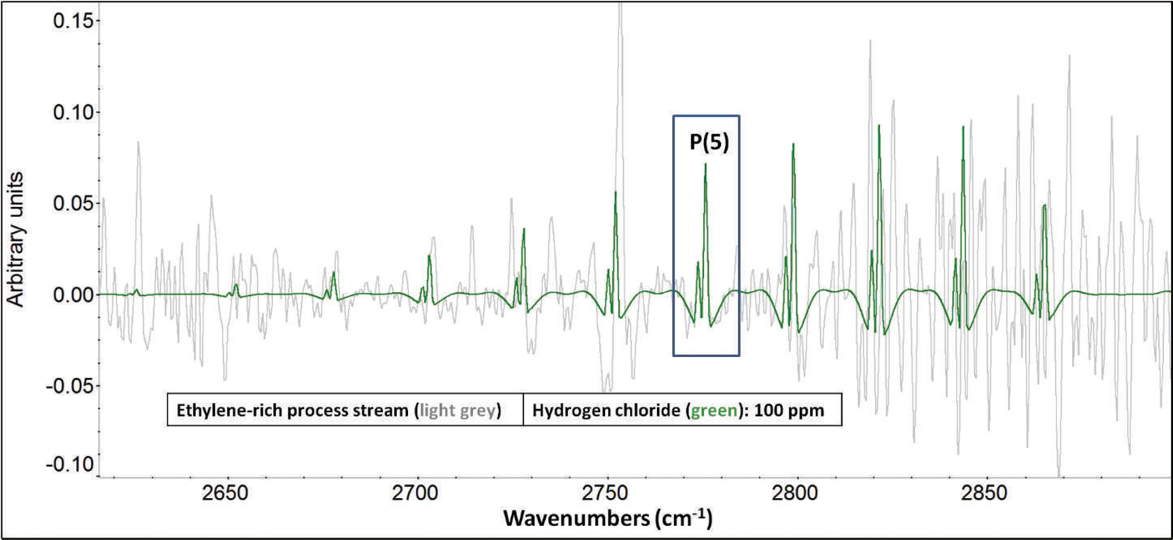
Overlap of spectra of the ethylene-rich process stream (gray) and HCl (green). Only the P(5) HCl line is suitable for use in the CLS model.

The total peak height of the P(5) HCl transition at 100 ppm concentration is 0.094. This results in a S/N of 28 for the ethylene-rich stream and 219 for the nitrogen-rich stream for a concentration of 100 ppm HCl. One can define the limit of detection as three times the noise. Given this, the limit of detection (LOD) for HCl in the ethylene-rich stream is approximately 10 ppm, and the LOD for HCl in the nitrogen-rich stream is 1.4 ppm.

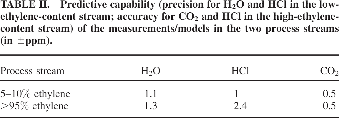
More importantly than looking at S/N, determination of analytical predictive capabilities in the two streams is based on measurement precision, or repeatability, under steady-state conditions. This provides information on how well the measurement can succeed at trending measurements and incorporates variations from sample system influences as well. Accuracies were determined in the best-case scenario with N₂ as a background gas under controlled laboratory conditions as discussed above, whereas in the process streams only precision could be determined. Precisions were calculated by assembling steady-state data over the course of 2 h (approximately 230 points for each stream) for each of the three components. Since the actual concentrations of the components differed between streams, precisions were estimated for each stream separately, with more variation observed in the ethylene-rich stream than in the nitrogen-rich stream. The measurements obtained for each component were analyzed using the JMP® Pro 9.0.1 software (SAS Institute) using individual measurements (IR) type control chart functionality with moving range (average) selected to provide the upper control limits (UCLs) for a 3-sigma level. A moving range average on a control chart is a calculation of how an input, in this case analyte concentration, changes from data point to data point. The larger the magnitude of the changes between points the less precise the analysis. Therefore, the goal would be to minimize the 3-sigma UCL on the moving range chart. In this case, the control chart for stream and analyte while the process was at steady state is used, and the 3-sigma UCL is used as a worst-case estimate for precision. In the ethylene-rich stream, the UCLs for precision for CO₂, H₂O, and HCl are 0.03, 1.3, and 2.4 ppm, respectively. For the nitrogen-rich stream, the UCLs for CO₂, H₂O, and HCl are 0.02, 1.1, and 0.37 ppm, respectively. The overall predictive capabilities of the system were determined by the worst of either the 3-sigma precision (for H₂O, and HCl in the ethylene-rich stream) or the accuracy (for CO₂, and HCl in the nitrogen-rich stream) and are summarized in Table II for the three species in the two different streams.

OPEN IN VIEWER

TABLE II.

Predictive capability (precision for H₂O and HCl in the low-ethylene-content stream; accuracy for CO₂ and HCl in the high-ethylene-content stream) of the measurements/models in the two process streams (in ±ppm).

Process stream	H2O	HCl	CO2
5–10% ethylene	1.1	1	0.5
>95% ethylene	1.3	2.4	0.5

As discussed previously, the interferogram centerburst intensity is indicated by the ptp voltage reading of the interferogram, saved as IgramPP by the analyzer software. It has been observed in practice that if the ptp voltages drop below approximately 1 V, then it is detrimental to the analysis—specifically of HCl—from an interference and baseline noise perspective. The ethylene-rich stream routinely operates in the range of 1–1.5 V ptp and to ensure it remains in this region, the cell was operated at a lower pressure and the sample cell temperature was increased to decrease the number density per unit volume of the ethylene, resulting in higher interferogram intensities. The range of IgramPP values increased from 0.7–1.2 to 1–1.5 V, resulting in the S/N discussed above. Operating conditions are discussed in more detail in the “Online Installation” section. During the course of around-the-clock operation, the IgramPP value was tracked as an indicator of measurement quality such that, if the reading dropped below 1V, the results were disregarded and the analyzer was checked for proper operation.

ONLINE INSTALLATION

The FT-IR analysis method itself is meaningless unless representative process samples can be delivered to it continuously and safely. As ethylene is a flammable gas, the area classification where the system is located is rated as Class 1, Division 2 Group C, and appropriate safety precautions for installation of electrical equipment are required. The FT-IR system was placed inside an analyzer building with appropriate climate controls, area classification, and monitoring/interlock/alarm systems.

Gas samples were delivered from sampling points in the process to the analyzer system using 0.6 cm (0.25 inch) stainless steel 316 (SS316) tubing lines. Heat tracing of the sample lines running from the process operations to the sample handling panel is critical for ensuring that moisture does not condense out of the vapor phase before analysis and that the partitioning of H₂O and HCl on sample system tubing walls is stable. As both H₂O and HCl are known to readily adsorb to tubing walls, ideally use of electropolished tubing or SilcoNert™ (SilcoTek, PA) type transfer tubing would be used in cases where response time is critical and bleed-over effects are detrimental. In this case, the application did not warrant this type of material. Response time results from the stream switching confirm that heat traced SS316 was suitable for this application. Heat tracing of the transport tubing also helped stabilize the temperature within the spectrometer. In this case, the temperature was controlled to approximately 60 °C and the pressure to approximately 1 psig. Typical flow rates through the analyzer were in the range of 1.2–2.5 L/min. The return sample gas was repressurized by a small pump and returned to the flare header. Appropriate process safety relief valves, interlocks, and alarms were implemented around the sample handling system.

In addition, since analysis of two distinct streams was required, automated stream source switching was implemented to allow use of a single FT-IR unit with a single sample cell. The automated stream switching system was devised using automated block valves (ABVs) and programming logic from the plant's distributive control system (DCS) to transition between the two streams every 10 min. Results from continuous operation show that analyte concentrations equilibrate in <4 min after stream switching. More details on observed response times are included in the “Results and Discussion” section. Analyzer results and alarms also are communicated back to the plant's DCS for real-time monitoring and could be used for real-time feedback control if desired. Typical communication protocols, such as RS232, Ethernet, and 4–20 mA signals, would be available.

RESULTS AND DISCUSSION

Before starting the process flow through the FT-IR, the full sample handling system and analyzer were rigorously leak-checked and purged for 24 h with dried plant nitrogen by connecting the nitrogen optics purge feed to the nitrogen-rich process stream on the sample handling system. The baseline concentrations of the three species being monitored were checked during the system purge with dried plant nitrogen for comparison with baseline results that had previously been obtained with laboratory nitrogen. These initial concentration measurements of the installed gas analyzer were found in good agreement with the observed laboratory offsets for HCl and CO₂. H₂O had a baseline offset of +3.3 ppm with the plant nitrogen in the field compared with the +1.3 ppm offset measured with laboratory nitrogen. This finding simply indicates a difference in quality of plant nitrogen from the two sources, and as it is installed in the plant, the plant offset was used in all subsequent measurements. As levels of H₂O in the process streams are consistently >50 ppm, this additional baseline contribution is considered negligible for the current application.

Figure 4 shows the trends of HCl, H₂O, IgramPP, and CO₂ in the nitrogen-rich stream over a five-day period, including a major process operation change after the first day. The spectrometer was fed with plant nitrogen at the beginning and end of this period. In between, it was sampling the nitrogen-rich process stream continuously. The system responded properly to plant changes, with the H₂O and CO₂ remaining within narrow bounds, but with the HCl increasing after an intentional change in operating conditions. The IgramPP was reading approximately 9 V with plant nitrogen and dropped to approximately 4.5 V with the nitrogen-rich process stream, indicating that the process measurements have a reasonable S/N as discussed above. There are well-known issues with HCl adsorbing to surfaces and smearing the measurements that were of potential concern due to the SS316 materials of construction of the sample system. In this case, the HCl measurements decreased rapidly to 0 once the plant nitrogen stream was fed into the instrument. In addition, during the time when the process stream was flowing through the instrument, changes in the HCl measurements reflected intentional changes in the process. All measurements returned to their original values after sampling was switched to plant nitrogen at the end of this 5 d period. These data indicate that the FT-IR setup provides meaningful results for the nitrogen-rich process stream.

OPEN IN VIEWER

Fig. 4.

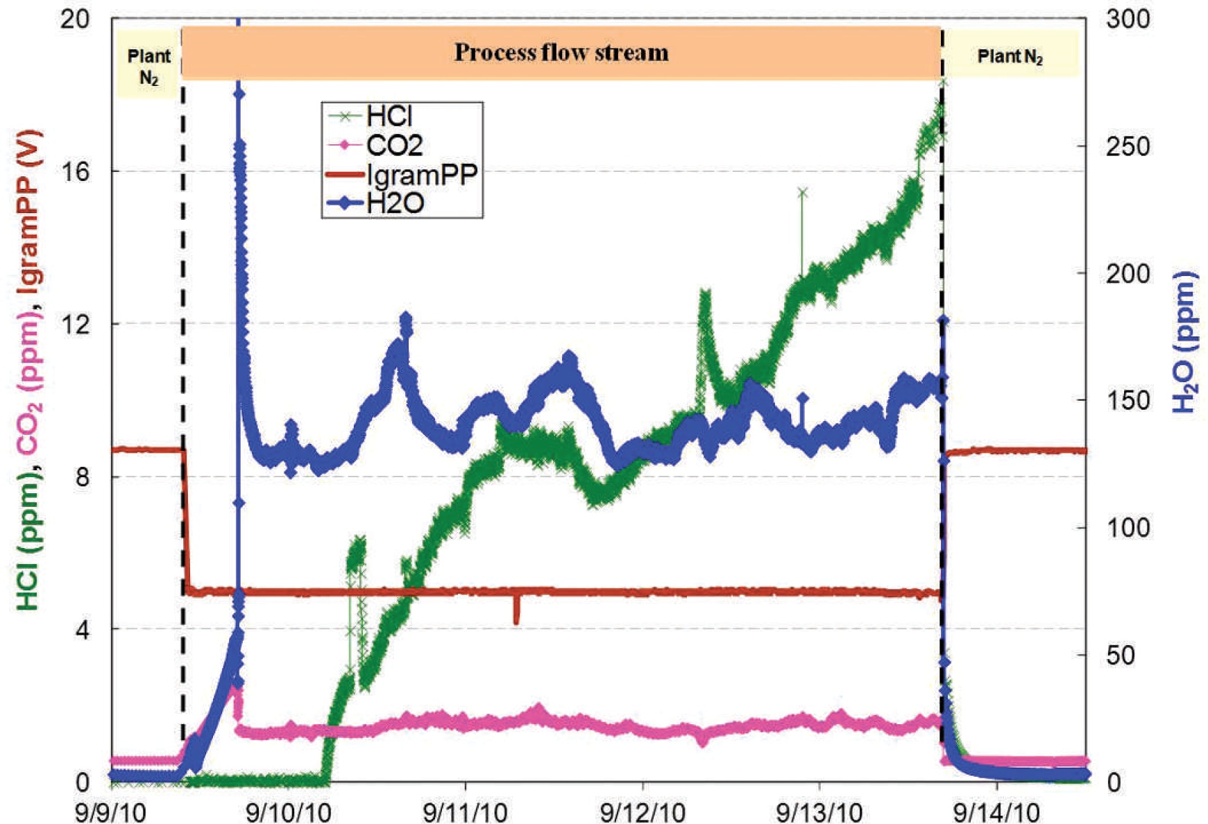
Trends of HCl, CO₂, IgramPP (left axis), and H₂O (right axis) at the nitrogen-rich process stream.

The ethylene-rich process stream contains >95% ethylene. As discussed above, it is not necessary to analyze for ethylene concentration to obtain results for the species of interest. Process monitoring of the ethylene-rich stream is shown in Fig. 5 for a 24 h period. As ethylene absorbs strongly in the regions of interest, the IgramPP voltage dropped by approximately 75% relative to the nitrogen-rich stream and remained at 1.5 V throughout the time the ethylene-rich stream was monitored. Sampling was switched to plant nitrogen in the middle of this period to verify that the instrument measurements returned to the expected values including the increase in IgramPP to approximately 8.5 V. The process underwent multiple changes during this period, and the measurements were able to reflect the changes.

OPEN IN VIEWER

Fig. 5.

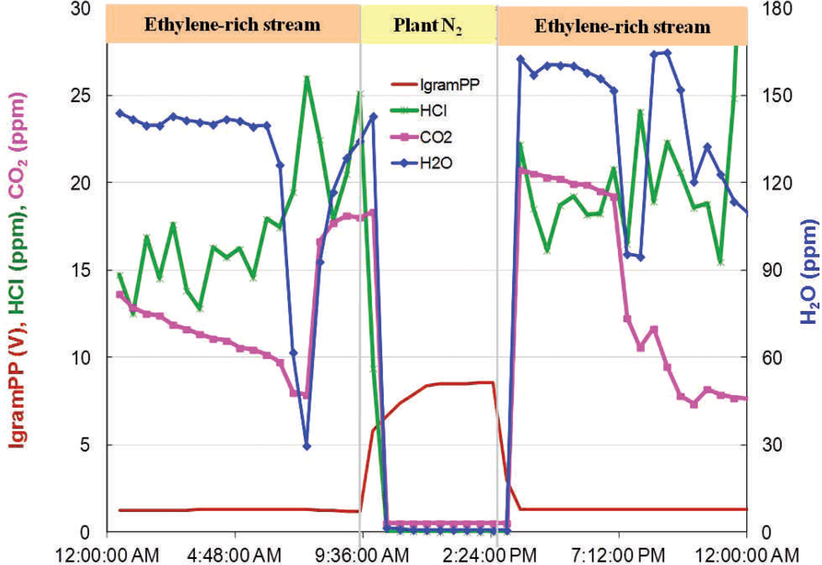
Trends of IgramPP, HCl, and CO₂ (left axis) and H₂O (right axis) at the ethylene-rich process stream with a period when plant nitrogen was flowing through the instrument.

A three-day monitoring period of the ethylene-rich stream is shown in Fig. 6. The data points shown reflect measurements every 30 min until the last half-day when they were obtained every minute. All species are seen in their near steady-state levels, and they undergo changes as the operations change. A more dramatic change is observed toward the end of this measurement period, when, after a process upset, HCl and H₂O values began increasing substantially over a 5 h period. IgramPP was at 1.5 V for most of this period, except for a few hours when it increased to 4.8 V as shown in the figure. Based on observation of raw spectra, specifically the ethylene transitions at 2569 and 3504 cm⁻¹, and knowledge of the nature of the process upset, this increase was attributed to a reduction of ethylene in the process stream.

OPEN IN VIEWER

Fig. 6.

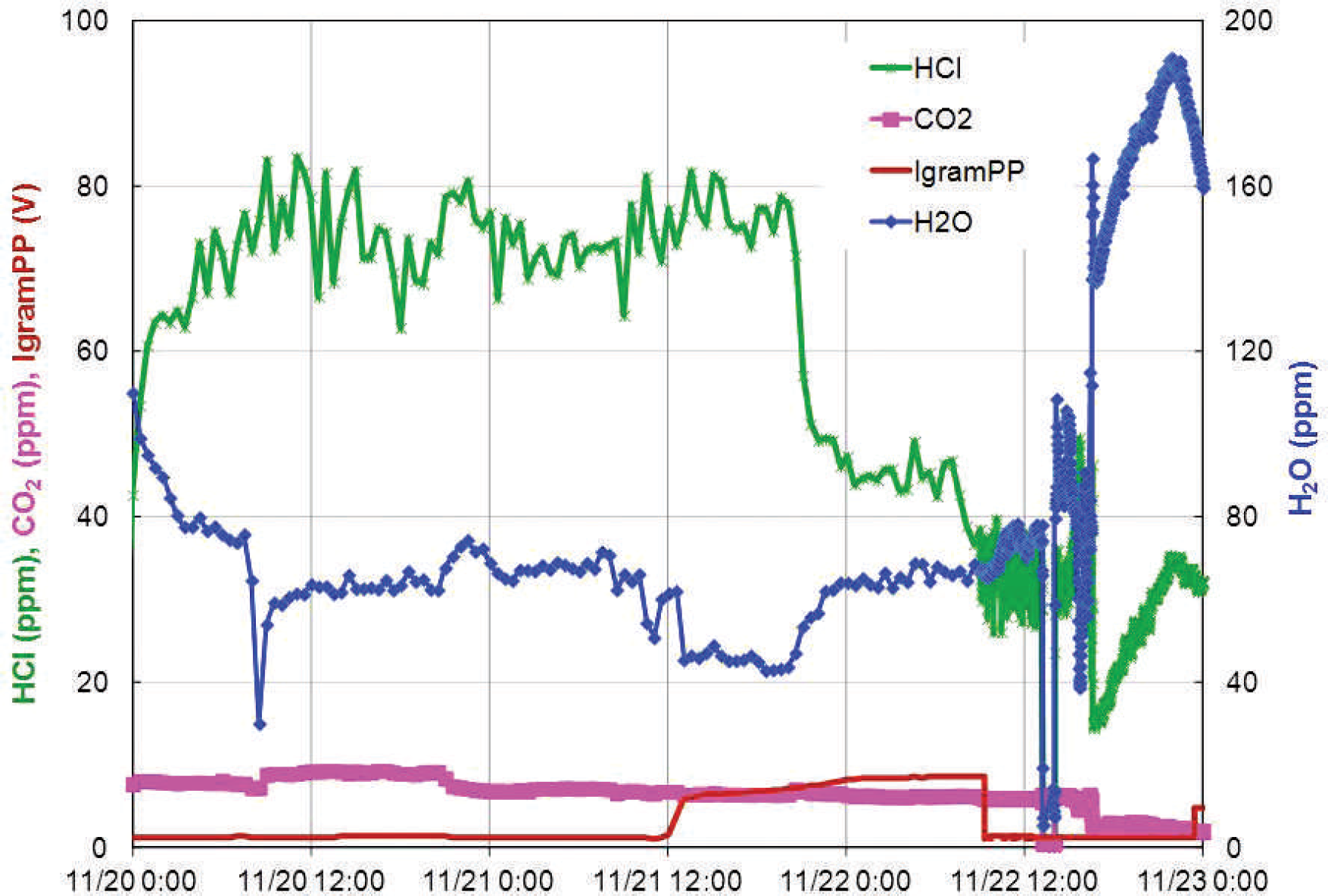
Trends of HCl, CO₂, IgramPP (left axis), and H₂O (right axis) at the ethylene-rich process stream for longer period during which the process was undergoing multiple changes.

During continuous online analysis, streams switch every 10 min between the nitrogen-rich and ethylene-rich streams. A 5 h snapshot of raw data shown in Fig. 7 clearly displays the differences in HCl, CO₂, and H₂O levels between the two streams and indicates that the measurements reach their steady-state values within the first 2–3 min after the switch in sampling occurs. Figure 7 also shows some variations with time in HCl and H₂O concentrations, reflecting intentional process changes. IgramPP ranged from 4.5 V for the nitrogen-rich stream to 1.5 V for the ethylene-rich stream, and as discussed above, the precision of HCl in the ethylene-rich stream is worse than in the nitrogen-rich stream (i.e., there is more deviation from data point to data point). Also, as discussed above, H₂O and CO₂ measurements do not have a poor precision issue as multiple peaks, which are better separated from ethylene interferences, are used to obtain the measurements.

OPEN IN VIEWER

Fig. 7.

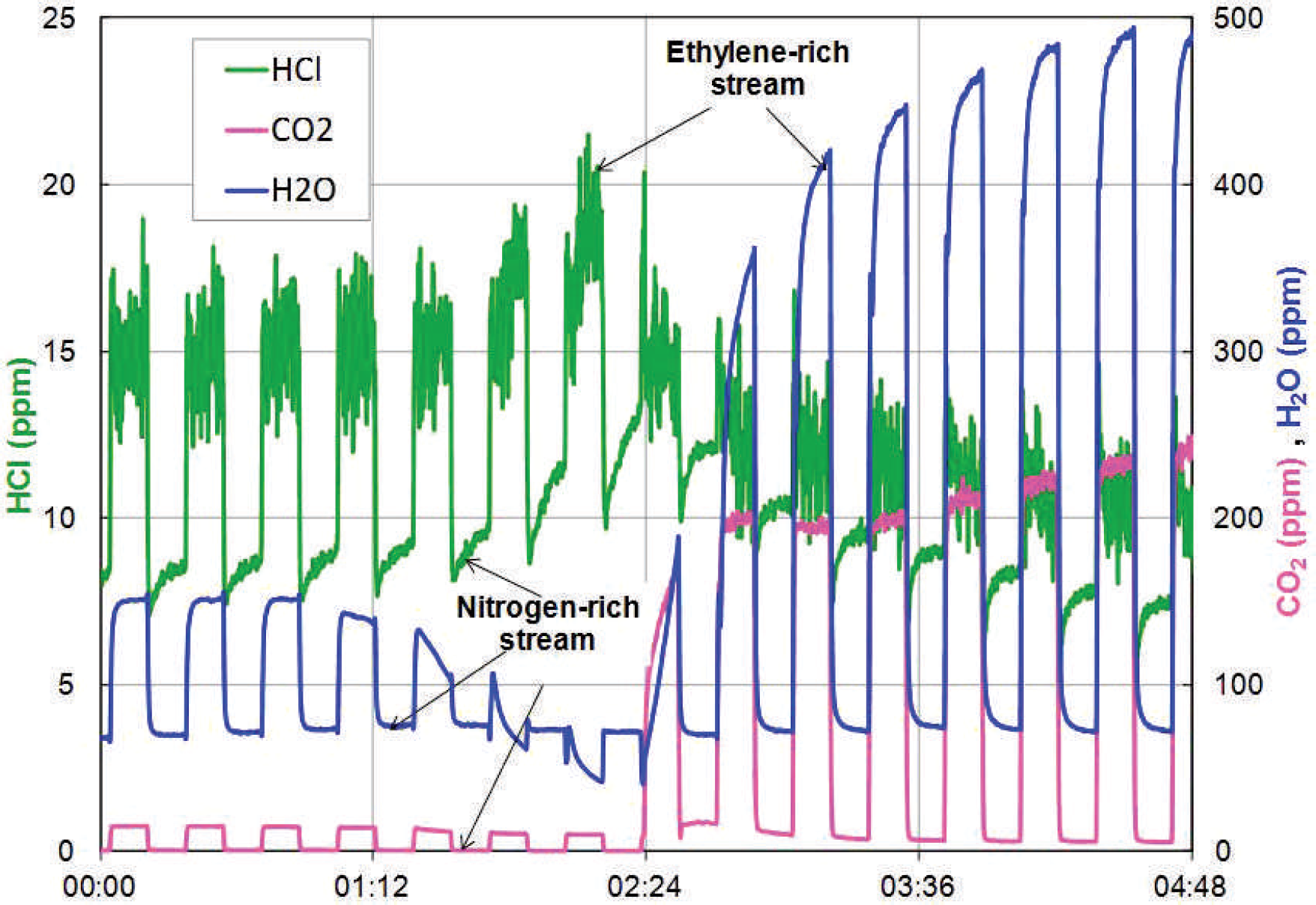
Trends of HCl (left axis), CO₂, and H₂O (right axis) as the sampling switched between the ethylene-rich and nitrogen-rich process streams for a period during which the process underwent intentional change.

Figure 8 shows process data for the two streams while the process is operated at steady-state. Data collection occurred every 15 to 16 s and stream switching occurred every 10 min. The data show how different components take slightly different lengths of time to equilibrate after a switch in the sampling stream, with HCl taking the longest, as it has the strongest adsorption to stainless steel surfaces. Therefore, when interpreting the data, the first 2–3 min after a stream switch were ignored and the measurements from the last 7 min before a stream switch were used to obtain process measurements with time. Equilibration of the HCl concentration took from 3 to 5 min depending on the magnitude of the concentration difference between the two streams and the direction the change, with decreasing HCl taking longer than increasing HCl, presumably due to wall adsorption in the sample handling system. CO₂ equilibrates much more rapidly (<1 min) and H₂O stabilizes in 1–3 min. All of these make sense from a wall adsorption equilibrium perspective. For HCl in particular, the most accurate readings were taken at the second half of the time spent on a given stream (i.e., the last 5 min before a switch). The value reported to the DCS for the purposes of control and decision making are 5 min average data from minutes 5–10 on a stream. Being that process changes are occurring on the order of hours, not minutes, this response time and averaging scheme are fully acceptable for this application.

OPEN IN VIEWER

Fig. 8.

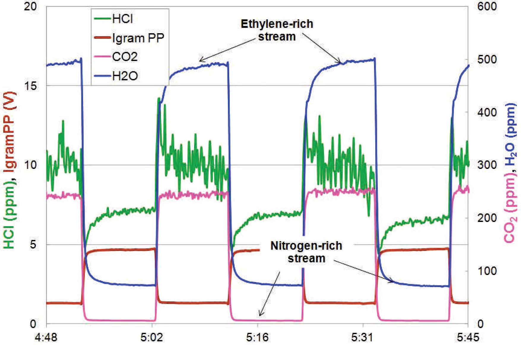
Trends of HCl, IgramPP (left axis), CO₂, and H₂O (right axis) as the sampling switched between the ethylene-rich and nitrogen-rich process streams for a short period during which the process was at steady-state conditions, showing the time it takes for measurements to reach steady-state values.

CONCLUSIONS

An FT-IR spectrometer with a long-path cell has been installed for online process analysis in a plant after taking into full consideration the safety precautions required. The system was used to successfully demonstrate monitoring of HCl, H₂O, and CO₂ concentrations at ppm levels in continuously flowing nitrogen-rich and ethylene-rich process streams. As ethylene absorbs in the region of interest, there are significant interference effects that had to be overcome. In the nitrogen-rich stream, implementation of the model was mostly straightforward and it produced robust results. To minimize ethylene interferences in the ethylene-rich process streams, some of the HCl peaks were not used in the CLS model, and only the P(5) rotational transition of the υ = 1 ← 0 was used to measure. Although this reduced the precision of the measurement, it nonetheless provided valuable information for monitoring the ethylene-rich process stream.

The advantages of using a rapid online analysis versus a periodic grab-sample method include improved ability to correlate to frequent process parameter changes, an increase in the number of simultaneously measured analytes, and a decrease in the exposure risks for operations personnel. As with any continuous online system, proper safety systems and operating discipline assure quality of the results and longevity of the analytical system.