Penetration of Light into Multiple Scattering Media: Model Calculations and Reflectance Experiments. Part II: The Radial Transfer

Abstract

In continuation of our contribution to “The Axial Transfer” (Appl. Spectr. 2012. 66(8): 934–943), this paper describes the distribution of localized incident radiation in multiple scattering layers of arbitrary thickness and analyzes the lateral intensity profiles of radiation leaving the sample from its illuminated and non-illuminated surfaces. The theoretical profiles are calculated with different approximations of the equation of transfer. We derive for both non-absorbing and absorbing layers simple analytical expressions and verify their accuracy and range of applicability by comparison with Monte Carlo simulations. Particular emphasis is given to the analysis of the radial absorption, an under-theorized and under-investigated feature that can help to identify weak or hidden absorbers. In addition, we contribute to the description of how the radial reflectance is affected by anisotropy or by error sources like multiple surface reflection for samples in glass cells or deflectance (sideway loss) of radiation in small samples. Finally, the theoretical results are compared with experimental data of radial reflectance for quasi non-absorbing and absorbing powder layers.

Keywords

Light scattering Light propagation Monte Carlo methods Reflectance spectroscopy Radial reflectance Radial absorbance

INTRODUCTION

The radial spread of radiation remitted from multiple scattering materials is of essential importance in high-resolution optical imaging. Examples are found in the fields of half-tone printings where the absorption of a pigment dot increases by acceptance of scattered radiation from outside the dot,^1,2 emulsion photographs where the formation of halos reduces the image contrast,^3,4 and tomography of buried objects where scattering controls the ultimate microscopic resolution.⁵

One begins to understand scattering of packed particles from basic electromagnetic theory.^6,–9 However, geometrical optics based on Chandrasekhar's equation of Radiative Transfer (CRT)^10,11 is still the most widely used approach to multiple scattering. Soon after publication, the model was applied to calculate the interaction with point or line sources of irradiation localized inside or at the surface of the diffuser.^12,13 The calculations were extended to collimated light beams penetrating the diffuser normal to the surface^14,–17 and the results were experimentally tested using e.g., fiber optics technology. Theoretically, the radial reflectance curves are mainly evaluated with the classical diffusion approximation of radiative transfer (DRT) or with a cubic lattice model using fixed mean scattering and absorption lengths.¹⁸ These methods deliver reasonable results for the far distance range. The near range needs more sophisticated solutions of CRT, which can be achieved e.g., by series expansion into higher order spherical harmonics,^19,20 by MC-simulations or by statistical photon density calculations.²¹ The importance of the near distance range becomes evident if one realizes that half of the lateral reflectance arises from optical distances σρ < 3 (for definition of symbols see Table I). Thus, the reflectance analysis of packed substrates with typical scattering coefficients of σ = 10² −10³ cm⁻¹ requires resolution beyond the limits of fiber optics. The corresponding equipment has been developed for medium²² and strongly²³ scattering materials.

TABLE I.

Definitions of some symbols

I_0c	intensity of collimated incident radiation
I_0d	intensity of diffuse incident radiation
θ₀, θ	angle of incidence, angle of light propagation, relative to the surface normal
μ₀, μ	cos θ₀, cos θ
z₀, z	layer thickness, depth coordinate inside the layer parallel to the surface normal
ρ0, ρ	radius of a cylindrical disk, radial distance from the principal cylinder axis
ρL	radius of the irradiated sample area
κ	absorption coefficient inside the layer / unit length
σ	scattering coefficient inside the layer / unit length
g= <μ>	anisotropy factor = average scattering cosine relative to incident μ′
σ_eff = (1 − g)σ	effective scattering coefficient / unit length
ε = (σ + κ)	extinction coefficient
ω = σ / ε	albedo
τ₀, τ = ε·z₀,ε·z	optical layer thickness, optical depth coordinate
χ	forward scattering ratio = scattering into the forward hemisphere / total scattering
S	Kubelka-Munk (KM) scattering coefficient / unit length,
	S = (3 σ_eff − κ) / 4
K	Kubelka-Munk (KM) absorption coefficient / unit length,
	K = 2κ
a = (K+S)/S b = (a² − 1)^1/2	parameters used in the Kubelka-Munk equations
T_cc	unscattered collimated transmission of collimated irradiation
T_cd	diffuse transmittance of collimated irradiation
T_dd	diffuse transmittance of diffuse irradiation
R_cd	diffuse reflectance of collimated irradiation
R_dd	diffuse reflectance of diffuse irradiation
R_int	internal reflection at the cylinder boundary surfaces
R_∞	diffuse reflectance of a layer with τ₀ → ∞ (semi-infinite layer)
D	deflectance = diffuse transmittance through the curved cylinder area at ρ = ρ₀, z < z₀
A	absorbed fraction of incident radiation, A = 1 − T − R − D
Φ	photon density inside the sample, normalized to incident photon flux density
P	probability that a photon reaches the maximum depth z_p
Ψ	probability that a photon resides at depth z inside the sample

In continuation of our contribution to “The Axial Transfer”,²⁴ this paper describes the distribution of localized incident radiation in multiple scattering layers of arbitrary thickness and analyzes the lateral intensity profiles of radiation leaving the sample from its illuminated and non-illuminated surfaces. The theoretical profiles are calculated with different approximations of the equation of transfer including deconvolution from the profile of the excitation source. These procedures are very elaborate and one of our main objectives is to find analytical approximations that are simple, but precise enough for practical applications. We especially emphasize the importance of signal detection with radial offset from excitation as a feature to discover buried species not only by diffuse reflectance absorption but also by Raman emission, for example.^25,26

The theory of radial absorption is not yet fully developed and we experimentally contribute to this field by the analysis of radial-resolved reflectance spectra. In addition, we contribute to the description of sources of errors like multiple surface reflection of samples in glass cells or deflectance (sideway loss) of radiation in small samples such as pharmaceutical tablets.

THEORY

Definitions, symbols, and most of the photometric equations are adopted from Part I.²⁴ In the interest of readability, we report the symbols in Table I as well.

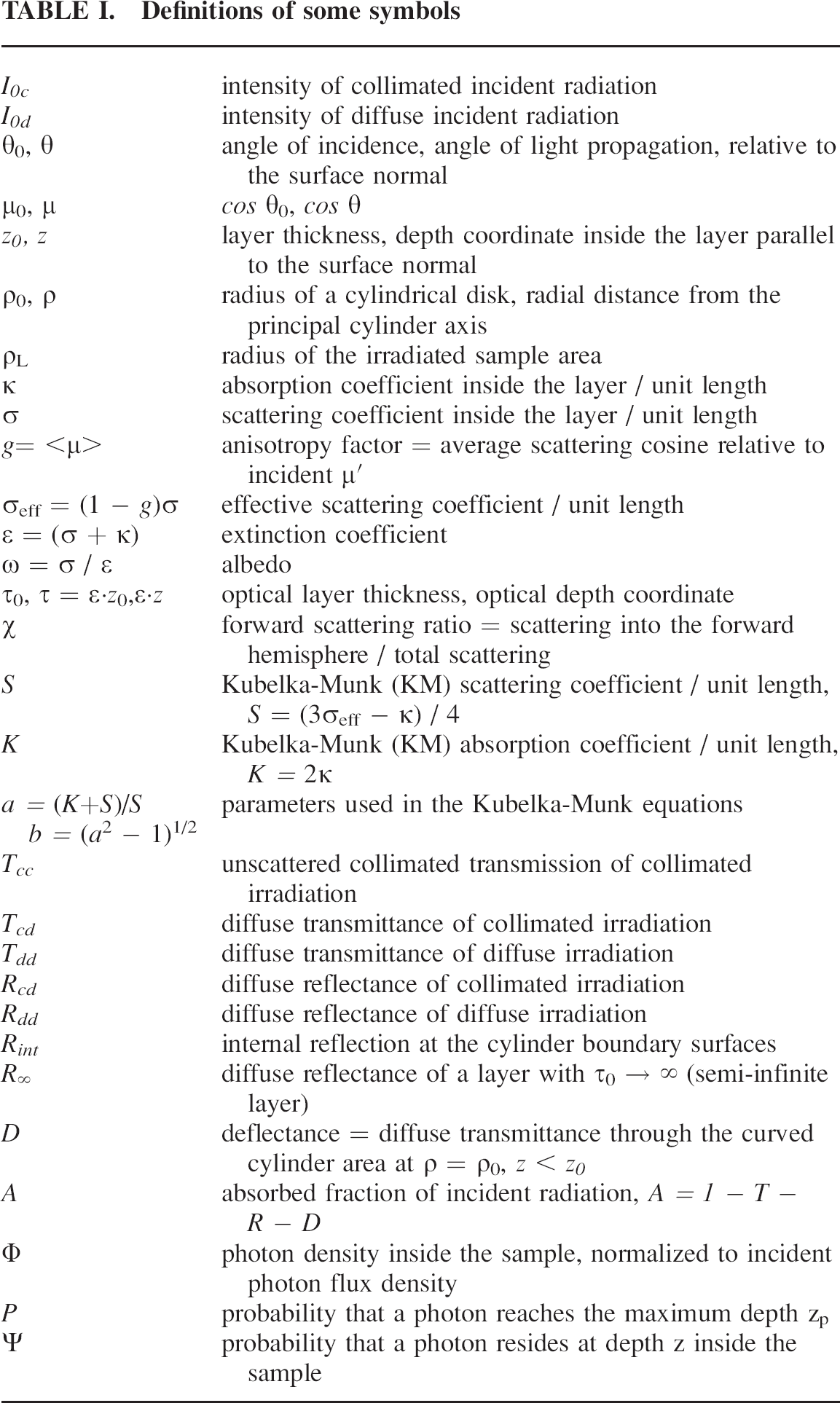
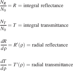
In the following section, the layer is irradiated with a narrow collimated or diffuse beam centered at ρ,z = 0. The reflectance (transmittance) is evaluated as a function of the distance ρ from the irradiation center. With N₀ = number of incident photons, and N_R (N_T) = reflected (transmittted) photons we use the following relations:

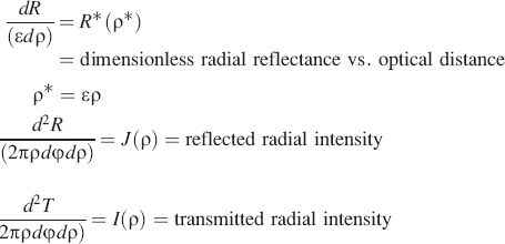
\begin{array}{l} \frac{N_{R}}{N_{0}} = R = intergral reflectance \\ \frac{N_{T}}{N_{0}} = T = intergral transmittance \\ \frac{d R}{d ρ} = R^{'} (ρ) = radial reflectance \\ \frac{d T}{d ρ} = T^{'} (ρ) = radial transmittance \end{array}

\begin{array}{l} \frac{d R}{(ɛ d ρ)} & = R^{*} (ρ^{*}) \\ = dimensionless radial reflectance vs . optical distance \\ ρ^{*} & = ɛ ρ \\ \frac{d^{2} R}{(2 π ρ d φ d ρ)} & = J (ρ) = reflected radial intensity \\ \frac{d^{2} T}{(2 π ρ d φ d ρ)} & = I (ρ) = transmitted radial intensity \end{array}

From Beer's law and geometrical factors, one obtains for the emitted (M) radial reflectance at distance ρ_M = (x_M² + y_M²)^1/2 from the center of excitation (X)

R^{'} (ρ) = \frac{σ ρ_{M}}{2} \int \frac{z}{r^{3}} Φ (ρ_{X}, z) exp (- ɛ r) d V_{X}

(1)

where Φ(ρX,z) is the photon flux density of primary and secondary excitations inside the layer as a function of the sample depth z and the radial distance ρX = (x_X² + y_X²)^1/2 from the axis of incidence, and $r = {[{(x_{X} - x_{M})}^{2} + {(y_{X} - y_{M})}^{2} + z^{2}]}^{1 / 2}$ . The integral spans the excited volume V_x of the whole layer. The radial transmittance T'(ρ) is obtained in analogy to Eq. 1 when the z-terms are replaced by (z₀ - z). Equation 1 assumes isotropic scattering and can be solved numerically, but only if the Φ(ρ_X,z) are known. The latter values are accessible in the simplest-however not very elegant–manner by Monte Carlo simulations. As example, Fig. 1 presents selected radiation densities in a non-absorbing layer of finite optical thickness. Very close to incidence, Φ falls off exponentially with e^−σz. For medium distances (σρ ≈ 1), Φ takes a z-dependence that is comparable to uniform irradiation (see Fig. 2 of Part I²⁴), and for far distances (ρ ≥ z₀), Φ is symmetrically distributed over the layer with a shape that corresponds to the probability density function Ψ of Eq. 16 or Fig. 3 of Part I.²⁴ This type of distribution is maintained with decreasing amplitude over the whole far distance range with the result that the radial reflectance becomes equal to the radial transmittance, $R_{ρ > z 0}^{'} (ρ) = T^{'} (ρ)$ . This symmetry is lost for absorbing layers where always $R_{ρ > z 0}^{'} (ρ) = T^{'} (ρ)$ .

Fig. 1.

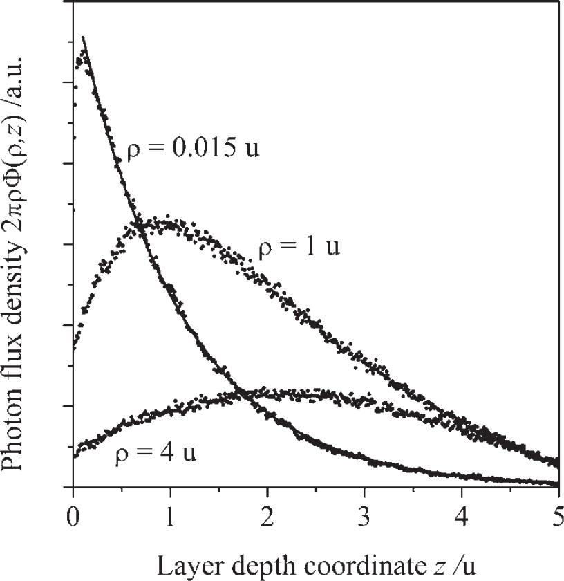
Selected photon flux densities 2πρ·Φ(ρ,z) as function of the sample depth z and the radial distance ρ from the axis of irradiation. Isotropic Monte Carlo simulations for a non-absorbing layer of thickness z₀ = 5 u, and scattering coefficient σ = 1 u⁻¹ (with u = arbitrary unit length). Number of incident photons N₀ = 5·10⁵. The solid line is the exponential fit of the curve at ρ = 0.015 u.

Fig. 2.

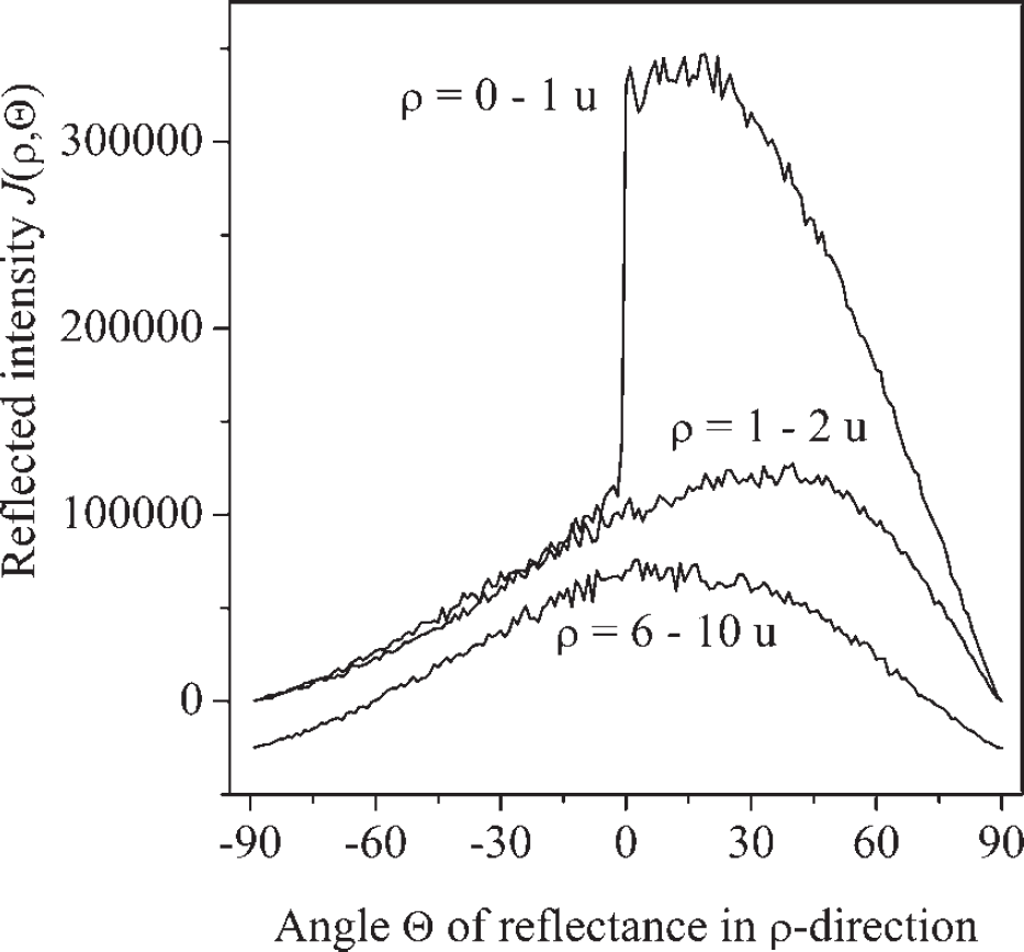
Angular resolved reflectance J(Θ,ρ) at different distances ρ from the axis of incident δ-irradiation. For clarity, the curve for large ρ is vertically displaced by −25 000 a.u. Isotropic MC-simulation with N₀ = 4.10⁷ photons.

Fig. 3.

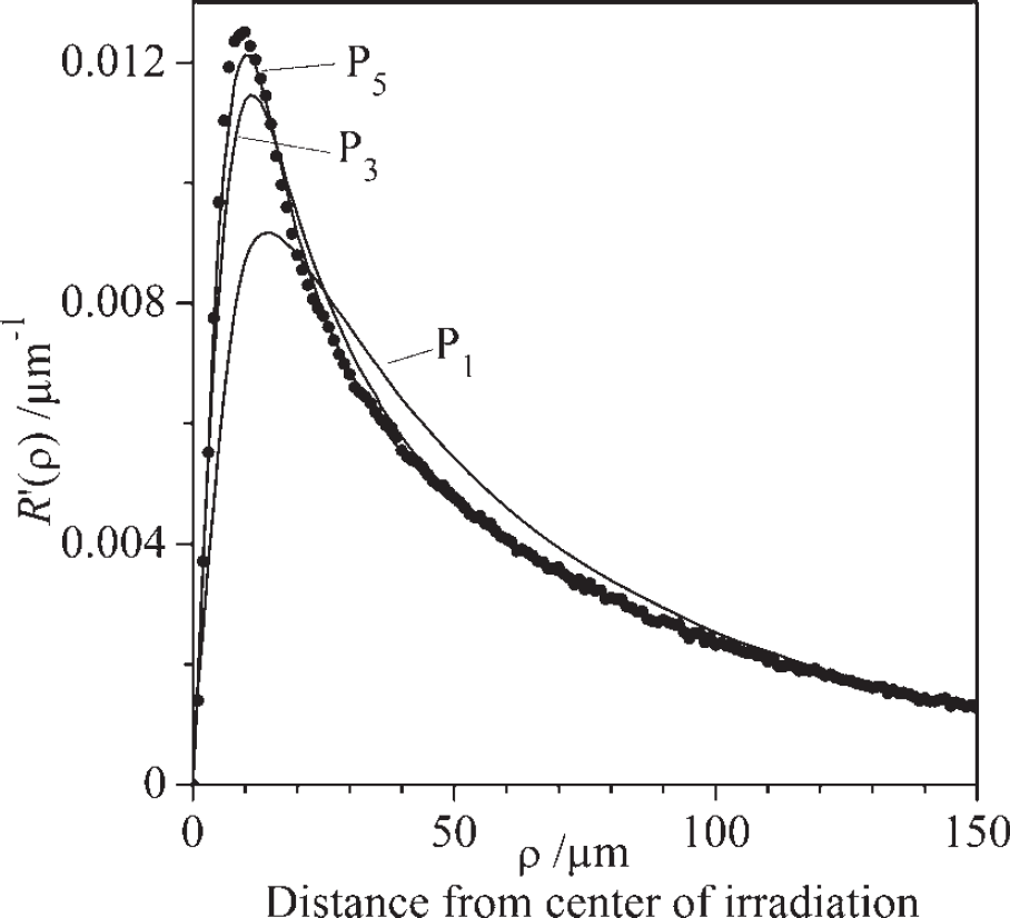
Radial reflectance R′(ρ) of a semi-infinite layer, σ = 300 cm⁻¹, κ = 3 cm⁻¹. Gaussian irradiation profile with e⁻²-half-width = 12 μm. Points: calculations with MC-simulation. Solid lines: P_L–approximations (L = 1, 3, 5) of the CRT-equation.

Some DRT-solutions of Eq. 1 are given e.g., for semiinfinite layers and normal incidence by different authors.^14,–17 A CRT-solution for arbitrary layer thickness is described in detail by Brun²⁰ applying transmission theory, transformation in the reciprocal space, convolution with the irradiation profile, and expansion into spherical harmonics up to P₅. The full analytical solution of Eq. 1 seems to be impossible. The mathematical problem arises from the near distance (nd) range, which is of extreme importance for the dot gain in halftone printings and the resolution limit in spectral micro-images. About 30% of the totally reflected photons leave the sample in the range of 0 < ρ* < 1 and additional 30% in the range of 1 < ρ* < 3.5 (values for non-absorbing optically thick layers; for absorbing or thin layers the fractions are even higher). In these ranges, the angular distribution of reflectance deviates extremely from Lambert's cosine-law as can be seen in Fig. 2.

The nd-range emits strongly into +ρ-direction. The far distance (fd) range with approximately symmetric angular reflectance begins not before ρ* > 5 and covers the last 25% of total reflectance. Thus, the classical diffusion model, which is a very good approximation for the description of axial radiation transfer upon uniform irradiation of the whole sample surface (see Part I²⁴), is not accurate enough to quantitatively reproduce the nd-range upon point irradiation. We overcame this limitation by expanding the symmetric P₁-approximation of Chandarasekhar's equation of radiative transfer, which is equivalent to the classical diffusion approximation, by additional odd P₃- and P₅-terms that consider the radial component of the Φ-gradient. As demonstrated in Fig. 3, the results are convincing. The figure compares the different approximations for a semi-infinite layer with optical parameters that are typical for packed powders used as pharmaceutical excipients or as white pigments. The high scattering power of the layer requires a focused laser as excitation source and microscopic lateral resolution so that the spatial extension of the source becomes clearly visible as the rising part of the R′(ρ)-curve. All approximations give equal results in the fd-range, whereas at short distances only P₅ comes close to the Monte Carlo curve that is considered as reference solution.

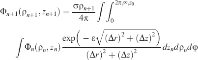
The P₅-expansion is mathematically very challenging especially if convolution with the radial profile of the excitation beam is included. However, one can solve the system via series expansion of the irradiated system into consecutive scattering processes. This method allows one to separate the total radial reflectance and transmittance into a sum of R′_n(ρ)- and T′_n(ρ)-curves emitted after n = 0,1,2, … ∞ scattering events, see Fig. 4.

Fig. 4.

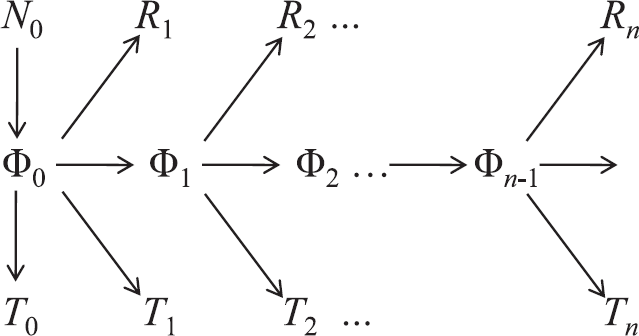
Separation of the total reflectance and transmittance in n consecutive scattering events.

Upon small spot irradiation (δ-irradiation) of normal incidence, where 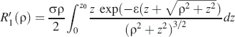$Φ_{0} π {(δ ρ)}^{2} / N_{0} = exp (- ɛ z)$ , one obtains for isotropic scatter

R_{1}^{'} (ρ) = \frac{σ ρ}{2} \int_{0}^{z_{0}} \frac{z exp (- ɛ (z + \sqrt{ρ^{2} + z^{2}})}{{(ρ^{2} + z^{2})}^{3 / 2}} d z

(2)

and

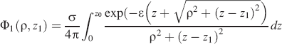
Φ_{1} (ρ, z_{1}) = \frac{σ}{4 π} \int_{0}^{z_{0}} \frac{exp (- ɛ (z + \sqrt{ρ^{2} + {(z - z_{1})}^{2}})}{(ρ^{2} + {(z - z_{1})}^{2}} d z

(3)

The radial transmittance T′(ρ) is equal to the right sides of Eq. 2 or Eq. 1 when the z²-terms are substituted by (z₀ — z)². Insertion of Eq. 3 into Eq. 1 yields R′₂(ρ) and T′₂(ρ). The terms of higher order are obtained with the recursion formula

\begin{array}{l} Φ_{n + 1} (ρ_{n + 1}, z_{n + 1}) = \frac{σ ρ_{n + 1}}{4 π} \int \int_{0}^{2 π, \infty, z_{0}} \\ \int Φ_{n} (ρ_{n}, z_{n}) \frac{exp (- ɛ \sqrt{{(Δ r)}^{2} + {(Δ z)}^{2}})}{{(Δ r)}^{2} + {(Δ z)}^{2}} d z_{n} d ρ_{n} d φ \end{array}

(4)

where ${(Δ r)}^{2} = ρ_{n + 1}^{2} + ρ_{n}^{2} + 2 ρ_{n + 1}^{2} ρ_{n} cos φ$ and ${(Δ r)}^{2} = ρ_{n + 1}^{2} + ρ_{n}^{2} + 2 ρ_{n + 1} ρ_{n} cos φ, and Δ z = Z_{n + 1} - z_{n}$ . All integrals have to be solved numerically with fast computers.

THEORETICAL SECTION

Approximate Analytical Radial Point Spread Functions. Insertion of σ, κ, into the MC-algorithm or into Eqs. 1 –4 leads to numerical representations of the radial reflectance and transmittance curves. For the inverse calculation of optical parameters from experimental curves, it is helpful to know analytical approximations that are precise enough for practical applications.

Non-absorbing layers. The simplest situation is met for the radial transmittance. Here, all points of emission are apart from the point of incidence by more than the layer thickness so that one can try to describe the radial dependency by a single exponential or Gaussian function. We found for non-absorbing layers

T^{'} (ρ, 0) = R^{'} (ρ, 0) \approx \frac{9 σ^{2} ρ}{{(1 + τ_{0})}^{2}} exp (\frac{- 3 σ ρ}{1 + τ_{0}}) T_{c d} (0)

(5)

where $T_{c d} (0) = 5 \cdot (1 - exp (- τ_{0})) + 3 τ_{0} / (4 + 3 τ_{0})$ is the integral diffuse transmittance of the layer upon normal incidence. This is because τ₀ = σz₀, the radial distribution of the transmittance depends mainly on z₀, and only a little on σ.

Figure 5 shows MC-simulations of three different layer thicknesses in comparison with the results of Eq. 5. The latter equation excellently describes the T′(ρ)-curves of layers with τ₀ < 8, whereas the curve maxima of thick layers are rendered at distances that are somewhat too short. In these cases, the exponential factor of Eq. 5 should be replaced by a properly normalized Gaussian with maximum at negative ρ-values. Equation 5 is valid also for the far-distance range ρ > z₀ of the radial reflectance. The amplitude of this exponentially decaying range decreases with increasing layer thickness and vanishes completely for semi-infinite layers. The near-distance range of R′ behaves completely differently. Here, the reflectance is mainly controlled by processes that are remitted after a small number of scattering events. These processes depend only very little on the layer thickness but strongly on the scattering coefficient. The range of σρ < 2.5 can be described with sufficient accuracy by the first ten terms R′₁–R′₁₀ of partial radial reflectances.

Fig. 5.

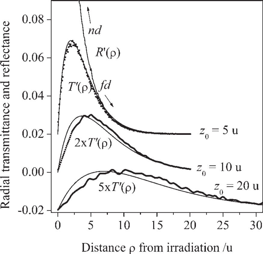
Radial transmittance and reflectance for three different layer thicknesses. Noisy curves: MC-simulations. Smooth curves: Analytical results according to Eq. 5. Neighboring curves are vertically displaced by 0.02 units.

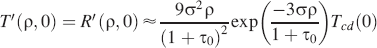
In part I we demonstrated for semi-infinite layers the proportionality between the mean values of penetration depth (MPD) and radial spread (MSR) of reflected radiation, see Fig. 9 and Eq. 22 of Part I.²⁴ We now use the penetration depth profile in the diffusion approximation, dR/dz_p = σ(T_cc + 1. 5T_cd)T_dd/2 and project it into the radial direction to obtain R′(ρ). The projection yields for non-absorbing layers and 8-irradiation

Fig. 6.

Radial total reflectance R′_tot and single scattered reflectance R′₁ of a nonabsorbing semi-infinite layer. MC-simulations (noisy, points) and analytical results according to Eqs. 6 and 2 (smooth, solid lines). For clarity, the results for diffuse incidence are vertically displaced by +0.1 reflectance units against normal incidence (μ₀ = 1). Presentation in general dimensionless coordinates.

Fig. 7.

Semi-logarithmic presentation of the radial reflectance as in Fig. 6 over a wider distance range. Noisy curve: MC-simulation. Smooth curve: DRT-projection of the depth profile into the radial distance direction.

Fig. 8.

Radial reflectance of non-absorbing layer against absorbing layer for z₀ = 100 u. Points: Monte Carlo simulations. Lines: Analytical approximations according to Eq. 8.

Fig. 9.

Diffuse reflectance spectra of a Gaussian absorption band vs. the detection distance ρ from the point of irradiation (z₀ = 20 u, σ = 0.3 u⁻¹, κ_max = 0.03 u⁻¹). The absorbance is referenced for the same distance σ outside the absorption band. Top: absorber is equally distributed over the sample depth. Bottom: same amount of absorber is concentrated in the central sample region at z = z₀/2.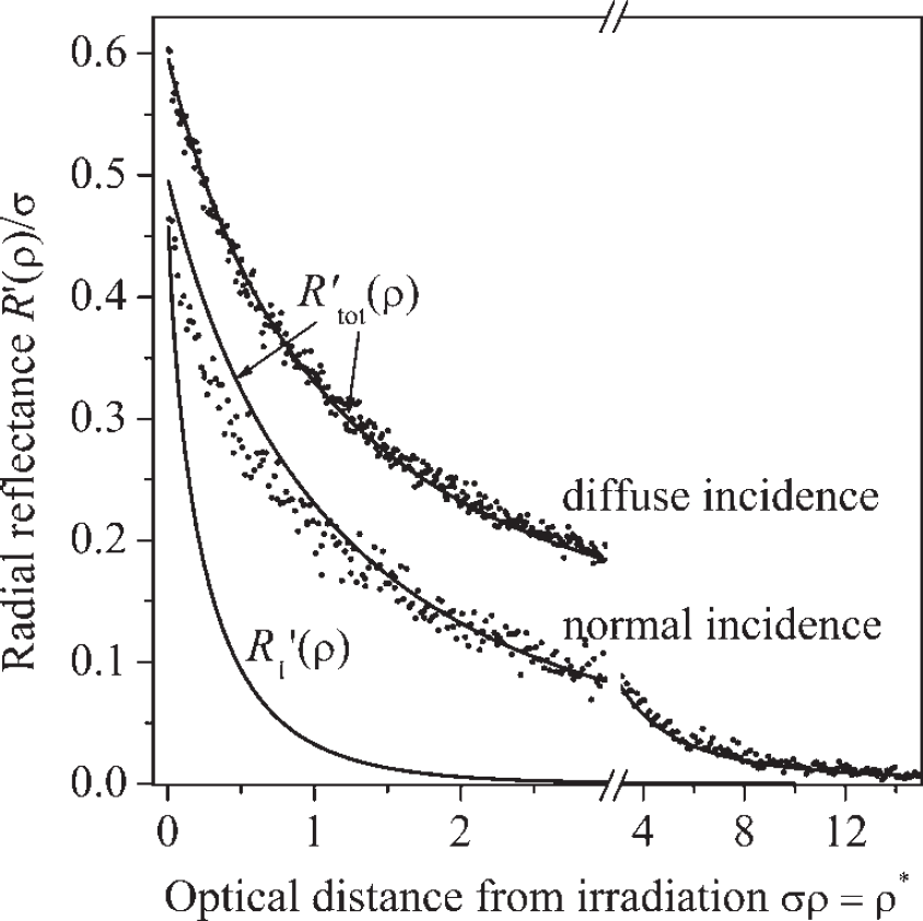

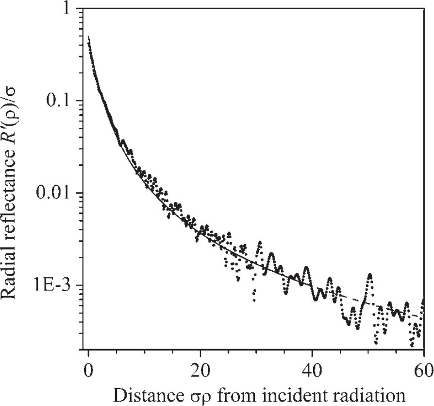
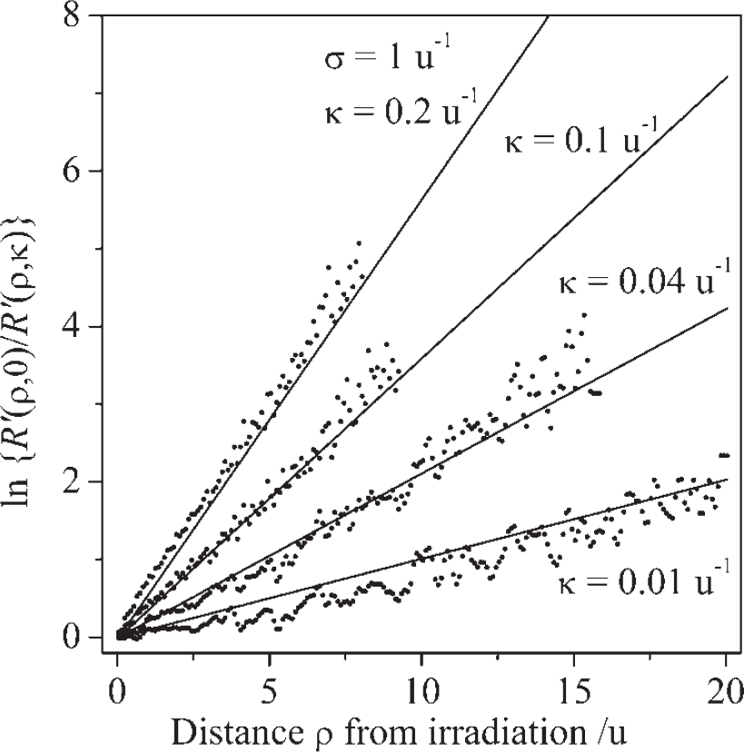
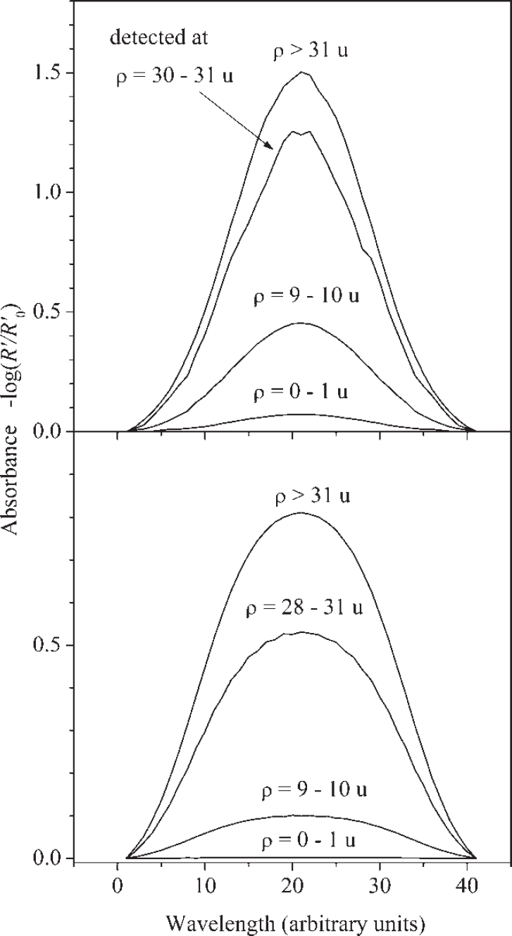
R^{'} (ρ, κ = 0) = \frac{σ (15 - (7 + 3 σ) e^{- σ ρ})}{{(4 + 3 σ ρ)}^{2}}

(6)

Figure 6 compares the result of Eq. 6 with MC-simulations. For diffuse irradiation, Eq. 6 is a perfect approximation. For normal irradiation, some differences are found in the near distance range σρ < 1. The range close to incidence is mainly controlled by R′₁(ρ) of Eq. 2, light that is backscattered and remitted directly from the incident beam, and this part of reflectance neither follows the diffusion equation nor Lambert's cosine law. The shape of R′₁(ρ) is also plotted in Fig. 6. In the very near distance range, the curve increases from zero to its maximum at σρ ≡ ρ* ≈ 0.004 (this range is not apparent in the figure because we quantize with ΔερG = 0.01 to avoid too noisy MC simulations). Then the curve decays with a final exponential of exp(−ρ*) and a pre-exponential factor proportional to (ρ*)⁻². Figure 6 starts approximately at the curve maximum. Here, the radial reflectance for normal incidence is determined to 95% by R′₁(ρ). The integral reflectance up to ρ* = 1 is determined to 50% by R₁. The total single scattered reflectance of non-absorbing thick layers amounts to $\int_{0}^{\infty} R_{1}^{'} (ρ) d ρ = 0.154$ and 0.195 for normal and diffuse incidence, respectively. In principle, R₁ is not much different from specular reflection. The signal arises from regions very close to the surface, carries only little information about absorption, maintains the polarization of the incident radiation, and is concentrated around a small angular aperture.

Figure 7 highlights the far distance range of the radial reflectance, where MC and Eq. 6 also produce equal results. It should be noted that the final slope of the radial reflectance is proportional to (ρ*)⁻², as obtained also for R′₁ from Eq. 1, which means that the reflected intensity is proportional to ρ⁻³. This result is in accordance with Farrell et al.¹⁶, whereas other authors^17,23 propose a final intensity slope proportional to ρ⁻².

Absorbing layers. The absorbance is proportional to κ and the path length λ of radiation inside the layer. The path length increases with the distance ρ from incidence and with σz₀. In practical situations, the radial reflectance of the absorbing layer, R′(ρ,κ) is measured as relative quantity against the non-absorbing reference R′(ρ,0):

\frac{R^{'} (ρ, k)}{R^{'} (ρ, 0)} = R_{r e l}^{'} = \frac{\sum_{i = 1}^{N_{R} (ρ)} exp (- k λ_{i} (ρ))}{N_{R} (ρ)}

(7)

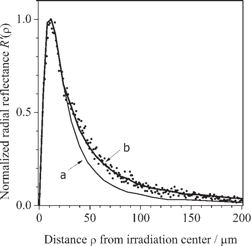
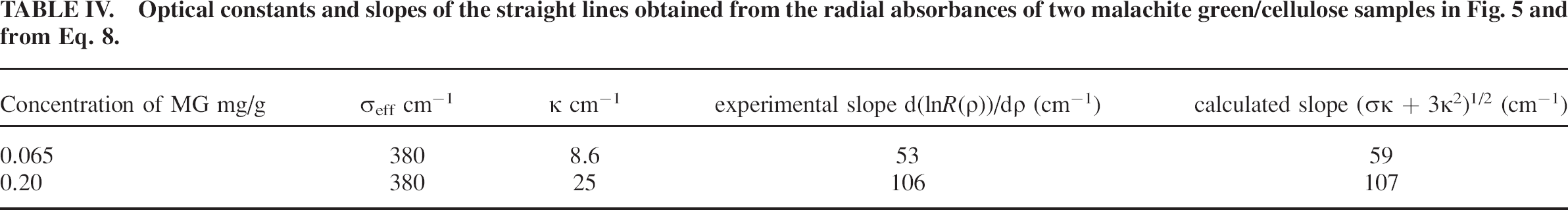
Because the individual path lengths cover a wide range (ρ < λ_i < ∞), Eq. 7 must be solved numerically or with the help of simplifying approximations. The simplest numerical solution is obtainable for R′₁, where λ_i(ρ) = z_i + (z_i² + ρ²)^1/2. The depth coordinate z_i of the first scattering event depends on ε⁻¹. Integration over z yields a convex curve of –ln(R′₁) versus ρ with a final slope of κ and a steeper initial slope that depends inversely on ε. The curves of the consecutive absorbances –ln(R ‘_n) extend to larger ρ and show decreasing convexity. For n > 10 the –ln(R′_n)-curves change into concave ones. The total absorbance curve -ln(R′_rel) is slightly non-exponential, especially for weak absorbers with albedos close to unity. For medium to strong absorbers the absorbance can be approximated by a single exponential.

Figure 8 depicts some results of MC simulations. The straight lines are analytical approximations of the MC-curves assuming the validity of one exponential equation

ln (\frac{R_{0}^{'}}{R^{'}}) = {(σ_{κ} + 3 κ^{2})}^{1 / 2} ρ

(8)

This equation describes with sufficient accuracy the first two decades of radial absorbance. It should be noted that this result is lower by approximately a factor 3^–1/2 than the attenuation coefficient $η_{ɛ} = {(3 σ κ + 3 κ^{2})}^{1 / 2}$ that is obtained with DRT or Kubelka-Munk inside a semi-infinite planar layer upon uniform irradiation of the whole surface or inside an infinite medium upon point irradiation. Equation 8 turns out to be an acceptable approximation also for finite layers of τ₀ ≥ 10.

The consequences of radially increasing absorption are presented in Fig. 9 for a Gaussian absorption band. The radial reflectance spectrum R′(ρ,κ) is referenced against the reflectance outside the band and the relative radial absorbance is plotted for selected distances from the incident δ-irradiation.

In Fig. 9, top, the absorber is uniformly distributed over z. Close to the region of incidence the absorbance is very low, because the path length of the remitted radiation inside the sample is short. With increasing ρ, the spectra gain more and more absorbance, but they lose their Gaussian shape somewhat in the log-presentation. So it is evident that laterally resolved absorption spectroscopy can help to identify weakly absorbing species. However, it is also evident that spectral imaging upon spot irradiation and detection of the same spot is not the best choice in strongly scattering media. In Fig. 9, bottom, the same amount of absorber is concentrated in a small Δz-layer at the z₀/2-center of the sample. Now the absorption close to irradiation becomes negligible because almost no light reaches the center of the layer. With increasing ρ the absorption depth increases and the absorption band becomes clearly detectable, although with a strongly distorted Gaussian shape. So laterally resolved absorption spectroscopy can help to identify hidden absorbers as, for example, in coated tablets.

Some Corrections for Real Systems. The model results of Eqs. 6 and 8 have to be modified for real systems regarding e.g., the radial spread of the irradiation source (see Fig. 3), the influence of anisotropic forward scattering, or internal reflections at the macroscopic sample boundaries.

Forward Scattering. Forward scattering is usually approximated by the average scattering cosine g and radial scaling with the effective scattering coefficient σ_eff = (1 − g)σ. This procedure becomes successful for the regions far apart from incidence. At near distances, the phase function of scattering enters the integral of Eq. 6 as a variable and reduces for g > 0 the contribution of R₁ and also of R₂ and R₃. The radial distribution of reflectance is shifted with increasing g to longer distances and forms, as shown in Fig. 10, for high g a maximum at ρ > 0. In this example the contribution of single scattered reflectance is reduced from the isotropic value (R₁,_iso = 0.154) to R₁ = 0.022, and the curve of isotropic scattering is reached not before optical distances σeffρ > 5.

Fig. 10.

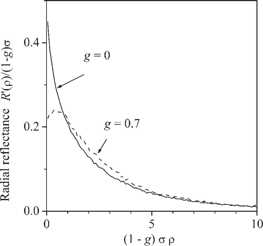
Radial reflectance of a non-absorbing layer, σ = 1 u⁻¹, z₀ = 10 u. Comparison of isotropic (g = 0, solid line) and anisotropic (g = 0.7, broken line) single scattering. Presentation in general dimensionless coordinates.

The anisotropy factor is classically determined from a combination of collimated and diffuse intensity measurements. The method is successfully applied to turbid media with low volume densities of scattering particles, typically embedded in a liquid phase. Examples are biological tissues, whole blood, or polymer micro-bead suspensions in water. The review of Cheong et al.²⁷ demonstrates that the anisotropies in those aqueous systems approach values of g > 0.9.

According to Mie calculations, we found that the maximum anisotropy of single spherical particles can be estimated by the approximation g_max ≈ m^−1/2 where m is the refractive index of the particle relative to the surrounding medium. Hence, the high g-values of solid/water dispersions are reduced in solid/air dispersions. In addition, forward diffraction is partly suppressed in packed systems by the close proximity of the particles. This effect further reduces anisotropy. We tried to determine anisotropy in powder layers by angular-resolved transmission measurements and extraction of the direct transmittance T_cc. The direct signals are extremely weak, even in very thin layers, and difficult to interpret because the effective scattering cross sections are mostly larger than the geometrical particle cross sections. Hence, direct transmission requires matter-free axial linear channels through the whole layer with diameters wider than the wavelength of light.

Instead of measuring T_cc, we propose for packed layers the evaluation of polarized radial reflectance as a function of the distance from the center of irradiation. Figure 11 presents the calculated g-dependence of the degree of polarization under the somewhat arbitrary limits that i) only the single scattered reflectance R₁ remains polarized, and ii) also R₂ and R₃ remain polarized to 50% and 25%, respectively. The calculations are compared in the Experimental Section with a real sample.

Fig. 11.

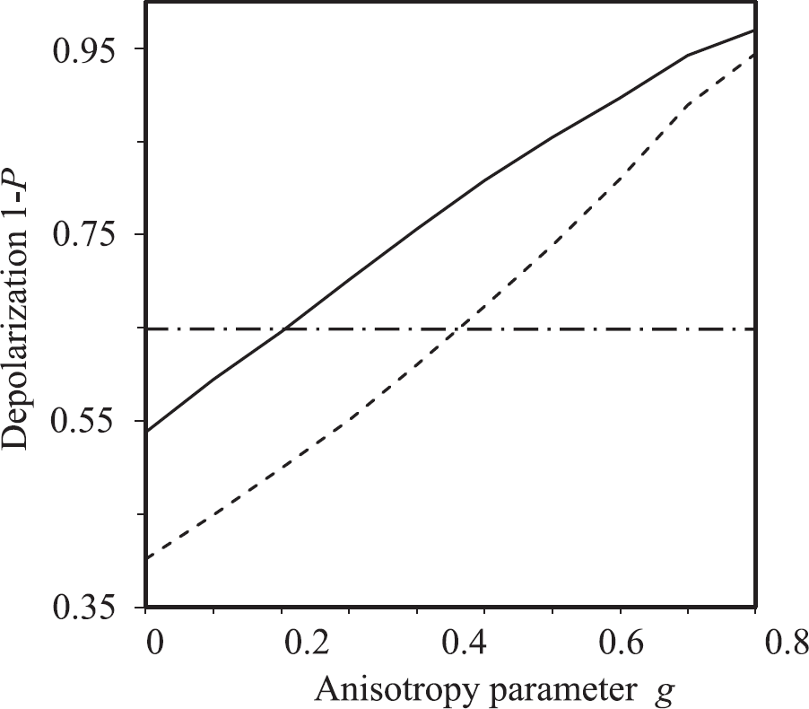
Depolarization of reflectance at distance ρ = 10 μm from the center of Gaussian spot irradiation (e⁻² w = 12.5 μm), σ_eff = 540 cm⁻¹, κ = 0.7 cm⁻¹. Solid line: MC simulation, where only R₁ contributes to polarization. Dashed line: R₁, and partly also R₂ and R₃ contribute. Dashed-dotted line: experiment on alumina powder layer.

Internal Reflection at the Macroscopic Sample Boundaries. Important cases of sample boundaries are

Samples with rough surfaces where no systematic long-range phase correlations exist between the scattered surface waves. Back reflection to the bulk remains unenhanced. Typical examples are uncompressed powders.

Samples with rough surfaces placed in optical cells. The cell walls enhance back reflection and radial spread. A typical value for the Fresnel reflection coefficient at the two boundaries of quartz glass is F = 0.18. This figure is obtained for diffuse internal irradiation and the assumption of a small air gap between the powder and the cover so that no total reflection occurs.

Samples with smooth surfaces like solid/liquid dispersions, liquid/liquid emulsions, super-gloss finish prints, etc. A large portion of the internal diffuse radiation is thrown back at the sample surface by total and partial Fresnel reflection; it can be estimated from the simple empirical approximation $F \approx μ_{T}^{2} + 0.1 (1 - μ_{T}^{2})$ is the cosine of the total reflection angle θ_T that depends on the refractive index n₂ of the dispersant or gloss finish against air. In most practical systems one obtains F = 0.45-0.6.

Scattering liquids like C) placed in optical cells with walls of thickness z_w. The amount of Fresnel reflection remains almost unchanged against case C), but the radial spread increases strongly because now reflection occurs mainly at the outer cell wall boundary.

The radial spread increases in the series A) < B) ≈ C) < D). Quantitatively, the mean point spread radius <ρR> of reflectance can be approximated as

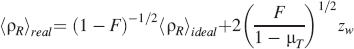
{〈 ρ_{R} 〉}_{r e a l} = {(1 - F)}^{- 1 / 2} {〈 ρ_{R} 〉}_{i d e a l} + 2 {(\frac{F}{1 - μ_{T}})}^{1 / 2} z_{w}

(9)

Figure 12 presents radial reflectance curves of a solid/liquid dispersion (σ_eff = 40 cm⁻¹) in a commercial optical cell of path length z₀ = 0.1 cm and cell walls of thickness z_w = 0.07 cm. Without surface reflection, the simulated curve a) yields the mean point spread radius of <ρR>_ideal = 470 μm. Addition of total surface reflection at angles μ < 0.7 (n₂/n₁ = 1.4) yields curve b) with <ρR>_real = 730 μm. Further addition of the cell walls yields curve c) with <ρ_R>_real = 2700 μm. The main contribution to the radial spread arises clearly from the cell walls, which act as quasi-light guides, and it should be noticed that curve c) extends to distances that can be longer than the dimensions of the cell so that part of irradiation is lost by deflectance.

Fig. 12.

Radial reflectance R′(ρ) of a thin layer with z₀ = 0.1 cm and scattering coefficient σ = 40 cm⁻¹. a) no internal surface reflection. b) total internal surface reflection at |μ_T | < 0.7. c) as b) but with additional glass covers of z_d = 0.07 cm.

Contribution of Deflectance. Laterally extended layers with ρ → ∞ are in practice not always available. In those cases it is important to determine how much of the incident radiation is deflected through the curved side area of the cylinder and not reflected and transmitted through the top and bottom planes, respectively. The deflectance D is calculated with the MC-algorithm of Part I²⁴ assuming circular cylinders of variable height, radius, and scattering coefficient. Only non-absorbing, isotropically scattering layers are considered, because in this case the unwanted deflectance is maximized.

The deflectance is logarithmically presented in Fig. 13 against the dimensionless optical cylinder radius σρ₀ with the optical layer thickness σz₀ as parameter. For easier reading, Table II shows some data in metric dimensions. Reliable R-and T-values are obtained only if D < 0.005 or, for higher precision, D < 0.001. This condition is feasible for thin layers (z₀ ≤ 0.1 cm) with sample radii of ρ₀ = 0.5–1 cm. Thick layers of z₀ ≤ 1 cm need larger sample radii with the experimental problem that the photometric spheres of commercial spectrometers do not offer wide enough sample ports to collect all R or T even if the condition of large sample radius is met. Medium scattering materials (σ ≥ 10 cm⁻¹) are especially susceptible to misinterpretation of R- and T-data. If the material is measured in a conventional UV/Vis-cell with z₀ = 2ρ₀ = 1 cm, the fraction of D can be very high (see Table II), especially in emulsions or solid/liquid dispersions where the cell windows with their high fraction of total internal surface reflection act as light guides for the enhancement of D.

TABLE II.

Diffuse deflectance D, diffuse reflectance R, diffuse transmittance T_d, and mean point spread radius <ρR> of a non-absorbing cylinder with scattering coefficient σ, cylinder thickness z₀, cylinder radius ρ₀. δ-irradiation at ρ,z = 0 in direction of the principal cylinder axis (μ₀ = 1).

σ	z ₀	ρ₀=0.5	ρ₀ = 1	ρ₀ = 2	ρ₀ → ∞	X
10	1	D = 0.327	0.115	0.010	0	<ρR>= 0.29
		R = 0.650	0.792	0.848	0.853
		T_d = 0.022^*)	0.092	0.142	0.147
	2	D = 0.349	0.189	0.060	0	<ρR>= 0.39
		R = 0.650	0.800	0.891	0.922
		T_d = 0.0003^*)	0.010	0.049	0.078
	0.1	D = 0.044	0.003	<10⁻⁴	0	<ρ₀ R>= 0.083
		R = 0.320	0.339	0.341	0.341
		T_d = 0.269*	0.290	0.291	0.291
100	1	D = 0.040	0.013	0.0008	0	<qR>= 0.063
		R = 0.958	0.978	0.984	0.985
		T_d = 0.002^*)	0.009	0.015	0.015

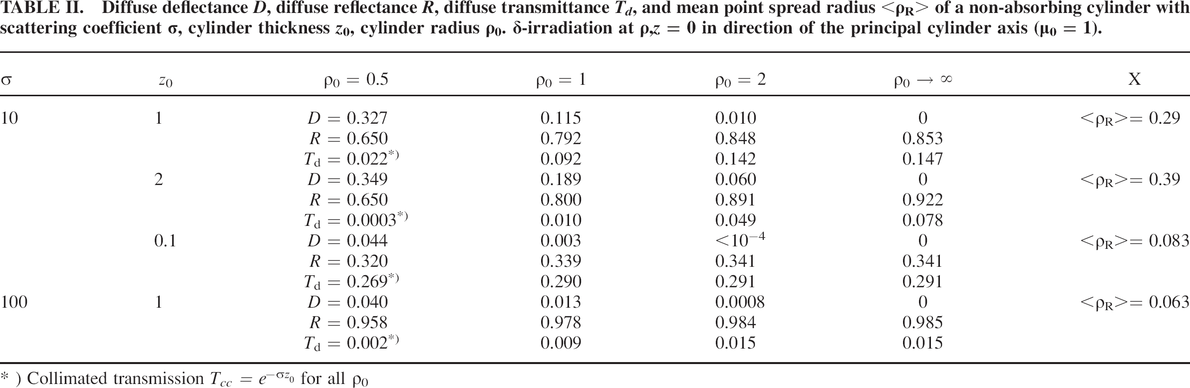
Collimated transmission T_cc = e^−σz₀ for all ρ0

Fig. 13.

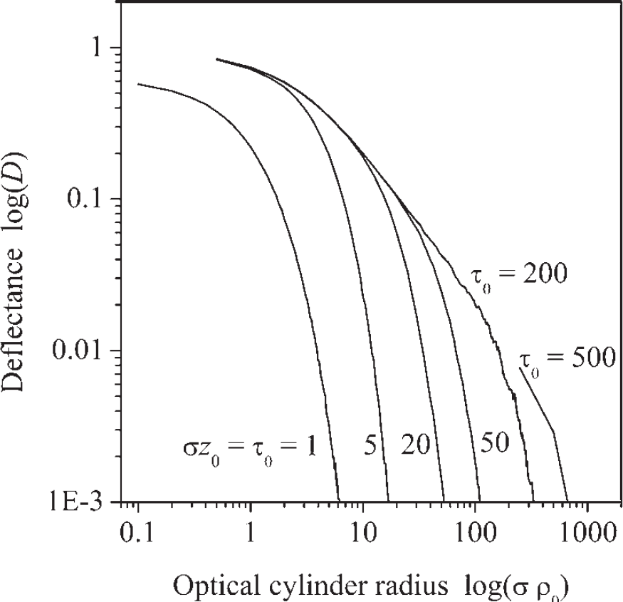
Deflectance of a nonabsorbing scattering cylinder upon δ-irradiation at ρ,z = 0, μ₀ = 1, as function of the optical cylinder radius σρ₀, with the optical cylinder height σz₀ as parameter.

EXPERIMENTAL SECTION

From Theory to Experiments. In the previous theoretical section we utilized Monte Carlo simulations to validate simplified analytical expressions for quasi non-absorbing and absorbing materials and to explore the influence of potential sources of error like side loss of radiation, anisotropy, and internal reflections on radial reflectance measurements.

In this experimental section we want to offer an exemplary overview of some practical applications of the theory on the systems considered in the previous section. With selected experiments we want to show how Monte Carlo simulations and the proposed simplified analytical expressions can help in the interpretation of experimental data, in the detection and prediction of chemical species, and in the estimation and correction of experimental errors.

First we present results of radially resolved reflectance measurements. Inverse Monte Carlo simulations, including the spatial extension of the irradiation source and analytical solutions, according to Eqs. 6 and 8, are used to extract optical parameters from quasinon absorbing and absorbing layers.

In the second part of the chapter we show experiments on potentially high error-affected systems. Inverse MC simulations will be used in this case for the indirect quantification of the Fresnel coefficients and anisotropy factors.

Experimental Setup. Experimental studies on powders were carried out by irradiating the samples at an angle of μ₀ = 0.985 with polarized He-Ne-laser light focused via a wide-angle objective to a spot radius of e⁻²-w = 12.5 μm. The same objective was used to produce an image of the reflectance pattern in a distance of ≈2 m. At this distance, J(ρ) was scanned using a photomultiplier + pinhole unit and lock-in amplification. The lateral resolution of the system was approximately Δρ ≈ 3 μm. In contrast to the model assumption of a scattering continuum, the real sample consists of small particles. Thus, the mean radial reflectance of coherent focused laser light is superimposed by random interference fluctuations (speckle patterns) that make accurate analysis impossible. We overcame this problem by z-rotation of the layer. In the case of liquid dispersions rotation was not required because the fluctuations smear out by Brownian motion.

Radially Resolved Reflectance Measurements. Quasi Non-Absorbing Powders. Figure 14 presents radially resolved reflectance curves of “white” powders with high scattering coefficients (σ_eff > 100 cm⁻¹). The R′(ρ)-data are shown in Fig. 14 in semi-logarithmic presentation. Neighboring curves are vertically displaced by 0.4 log-units. From the integral reflectances R_tot ≈ R_∞ and back simulation of the R′(ρ)-curves with the P₅-approximation or MC-simulations we obtained the scattering and absorption coefficients of the layers (see Table III). The R′(ρ)-curves are modified in the near distance range by the spatial extension of the laser (compare also Fig. 3): the back simulations were started in the far distance range and the data were refined in the near distance range by incorporating the radial laser profile and the anisotropy according to Eq. 11 of Part I.²⁴ However, the anisotropy factors of the packed powders were low (g < 0.55, as example see Fig. 17 and the associated text) so that no reliable differences from isotropic scattering could be observed.

TABLE III.

Scattering coefficients, absorption coefficients, and spot spread radii of “white” powder layers obtained from radial resolved reflectance measurements at λ = 633 nm with laser irradiation focused to a Gaussian spot of e²-width = 12.5 μm.

Substrate	σ_eff/cm⁻¹	κ/cm⁻¹	<ρ_spot>/μm	grain diameter/μm
filter paper¹	σ_‖ = 220	0.15	169	a = 1–2 mm
	σ_⊥ = 360			b = 40 im
cellulose powder²	380	0.19	122	20–30
alumina³ (Al₂O₃)	540	0.45	79	2–8
magnesia (MgO)	835	0.09	59	3–5
fluorite (CaF₂)	1240	0.25	47	<1
barium sulfate (BaSO₄)	1940	0.39	28	<1
zinc oxide (ZnO)	3170	0.63	20	<1
rutile (TiO₂)	4550	0.90	15	<1

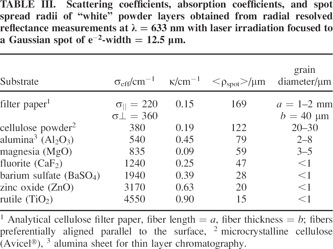
Analytical cellulose filter paper, fiber length = a, fiber thickness = b; fibers preferentially aligned parallel to the surface

microcrystalline cellulose (Avicel^®)

alumina sheet for thin layer chromatography.

Fig. 14.

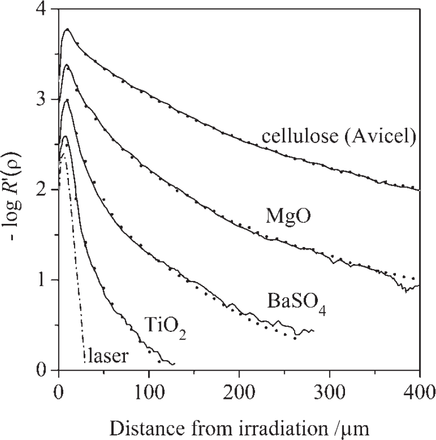
Experimental (lines) and back simulated (points) radial reflectance curves of some white pigments. Irradiation at λ = 633 nm, detector aperture ν = 23°. Neighboring curves are vertically displaced by 0.4 log-units.

Fig. 15.

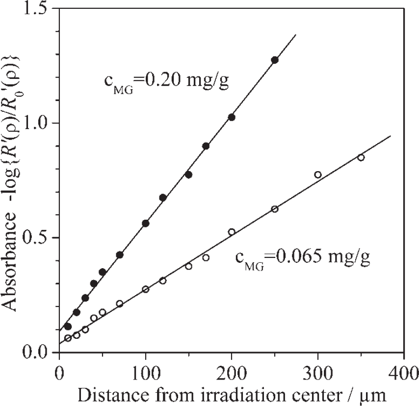
Radially resolved absorbance curves (λ = 633 nm) of microcrystalline cellulose (Avicel®) dyed with different loadings of malachite green (MG) as given in Table IV. Reference: undyed cellulose.

Fig. 16.

Radial reflectance curves of printing paper, focused laser irradiation at λ = 633 nm with e⁻²-half width = 12.5 μm. a) bare paper. b) same paper covered with polymer laminate of thickness z_w = 4 μm. Monte Carlo simulations (points) of both curves yield σ = 1050 6 50 cm⁻¹, κ = 0.3 cm⁻¹ and an additional internal Fresnel reflection coefficient F = 0.6 for the laminate.

Fig. 17.

Polarization-dependent radial reflectance for packed alumina particles. Solid lines: experimental values. Dotted lines: MC simulation.

A special situation was met in filter paper, where the cellulose fibers are preferentially oriented with their long axes parallel to the paper surface. Thus one expects different scattering coefficients in axial and radial directions. We were able to analyze this type of anisotropy by R′(ρ)-curves as function of the layer thickness.

Absorbing Powders. The influence of absorption on the radial reflectance R′(ρ) was studied with the dye malachite green (MG) adsorbed on microcrystalline cellulose powder. The powder was suspended in n-hexane solutions of MG, wherefrom quantitative adsorption took place, and afterwards dried at slightly elevated temperatures. Most of the photometric results were already presented in Table V of Part I.²⁴ Next we concentrate on the radial absorbance to compare the experiment with the model calculations of Fig. 8 and Eq. 8. The absorbances of two dye loadings are plotted in Fig. 15 as a function of the distance ρ from irradiation. Both concentrations result in straight lines. Table IV compares the experimental slopes with the results of Eq. 8. The excellent correlation is evidence for the practical applicability of Eq. 8.

TABLE IV.

Optical constants and slopes of the straight lines obtained from the radial absorbances of two malachite green/cellulose samples in Fig. 5 and from Eq. 8.

Concentration of MG mg/g	σ_eff cm⁻¹	κ cm⁻¹	experimental slope d(lnR(ρ))/dρ (cm⁻¹)	calculated slope (σκ + 3κ²)^1/2 (cm⁻¹)
0.065	380	8.6	53	59
0.20	380	25	106	107

TABLE V.

Radiation intensities emitted at λ = 800 nm from multiple scattering samples (d = particle diameter) in quartz cells of different thicknesses z₀. R_exp = experimental reflectance through the illuminated window, T_exp = experimental transmittance through the rear window, D = deflectance through the side windows. Spectrometers: Lambda 9 and 1050 (Perkin-Elmer) equipped with photometric spheres. The experimental sum of all three emission processes (fifth column) was measured with the samples in the center of the photometric sphere. Reflectance reference: Spectralon^®.

Sample in optical quartz cell h × w × z₀ = 3 × 1 × z₀ cm³ window thickness z_w = 0.08 cm	R _exp	T _exp	R_exp + T_exp	(R + T + D)exp	σ_eff/cm⁻¹
alumina powder, d = 45 nm z₀ = 0.1 cm	0.75	0.18	0.93	0.98	87
alumina powder, d = 45 nm z₀ = 1 cm	0.85	0.003	0.85	0.98	87
polystyrene beads, d = 802 nm 1 % w/w in aqueous suspension z₀ = 0.1 cm	0.48	0.32	0.80	0.99	28

From Ideal to Real Systems. Influence of Internal Surface Reflection on the Point Spread Radius and on Deflectance. The contribution of (Fresnel) reflection at the layer boundaries was investigated in combination with deflectance. Figure 16 shows as example the influence of a thin non-scattering polymer laminate (z_w = 4 μm) on the radial reflectance of a high quality printing paper. Without laminate, the R′(ρ)-curve at λ = 633 nm can be fitted well with σ_eff = 1050 6 50 cm⁻¹ and a residual absorption coefficient of κ = 0.3 cm⁻¹. After lamination, the reflectance extends to longer distances. The fit with fixed σ_eff- and κ-value yields internal Fresnel reflection of F = 0.6. This is a reasonable value for intimate paper/laminate contact that gives rise to almost diffuse internal illumination of the outer laminate boundary and thus a lot of total back reflection. The thickness of the laminate is in this case of negligible influence. However, the situation changes completely when the samples are covered with a thick non-scattering layer of a glass window.

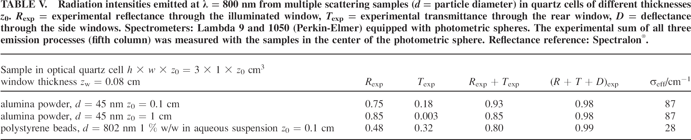
Table V presents results of three medium scattering samples measured in commercial fluorescence cells. The experimental (exp) data were obtained with photometric sphere equipment in the standard sample positions for transmittance T_exp and reflectance Rexp. In addition, the samples were placed in the center of the sphere to detect the sum of all contributions (R + T +D)_exp to re-emission. All samples show significant contributions of deflectance in the range of D = 0.05–0.2. Simulations for the uncovered samples yield much smaller values, extending partly below the plotted range of Fig. 13 (D < 10⁻³). Thus the high experimental values must be the consequence of radiative transport within the glass windows. Correct reflectance and transmittance data are measured in those cases only with large area cells and photometric macroequipment. For less accurate estimates one can also use internal normalization outside the absorption range with R_true ≈ R_exp/(R_exp + T_exp) and T_true + R_true → 1.

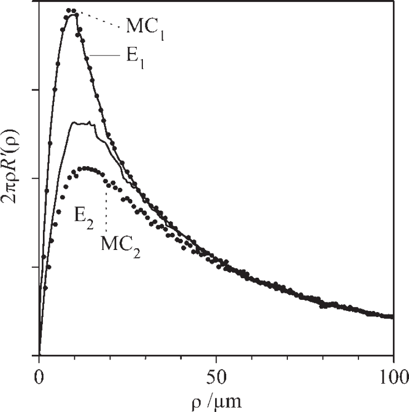
Polarized Reflectance Versus Distance from Incidence; Approach to Anisotropy of Scattering in Packed Powders. A layer of packed alumina particles with diameters d = 2–6 μm was irradiated in z-direction with a focused laser beam polarized in y-direction. The reflectance was scanned in x-direction using a second polarizer oriented either in y-direction (parallel, R_||) or in x-direction (perpendicular, R_⊥).

Figure 17 presents two experimental curves, E₁ = R′_|| + R′_⊥ and E₂ = 2 R_⊥, as well as simulated data for isotropic scattering MC₁ = R′_tot and MC₂ = R′_tot − R′₁. The experimental degree of polarization P = 1 − (E₂/E₁) amounts at the center of irradiation to Pmax = 0.48. This value decreases with increasing × and approaches zero for x > 30 μm. The E₁-curve can be well fitted with an effective scattering coefficient and a small residual absorption coefficient, resulting in MC₁. From these coefficients, R′1 and finally MC₂ were calculated, assuming isotropic scattering. It can be clearly seen that E₂ > MC₂. Hence R′₁ is not fully polarized or, much more realistically, forward scattering reduces its contribution to total reflectance. Figure 11 shows the correlation between forward scattering and the resulting depolarization of reflectance. The experimental data of the alumina layer yield an anisotropy factor of g = 0.25 if only R₁ is assumed to be polarized. However it is reasonable to consider also the higher orders n + 1 of reflectance as partly polarized according to P_n+1 = αP_n, where α = 0.7 for Rayleigh-spheres²⁸ and α = 0.65-0.8 for Miespheres.²⁹ Irregular particles tend to stronger depolarization³⁰ as well as particle aggregates.⁶ In Fig. 11 we weighted the polarization of higher order reflectances with α = 0.5. Thus, the anisotropy of the alumina particles lies in the range of g = 0.25-0.5. This value is still moderate and allows one to apply the concept of effective scattering also in the field of laterally resolved reflectance.

CONCLUSIONS

Monte Carlo simulations and analytical approximations for the radial propagation of light are presented and discussed.

The calculations show a substantial difference between far and near distance range. Close to the region of incidence the reflected light undergoes mainly single-scattering processes. The signal arises from regions very close to the surface, carries only little information about absorption, maintains the polarization of the incident radiation, and is concentrated around a small angular aperture

For non-absorbing species the derived approximations are accurate enough for the transmittance and for reflectance in the far distance range, but they fail in the near and very near distance range.

For absorbing species, the absorbance increases radially with approximately exponential slope. So it is evident that laterally resolved absorption spectroscopy can help to identify weak or hidden absorbers.

In the analysis of real samples, the influence of anisotropic forward scattering and internal reflections lead to an increase of the radial spread of reflectance

The close agreement between the theoretical and experimental data confirms the validity of the model and of the assumed approximations.

Footnotes

AKNOWLEDGMENTS

For part of the work we acknowledge the financial support of the Federal Ministry of Education and Research (BMBF) and the German Research Foundation (DFG).

References

Yule

Nielsen

. The Penetration of Light into Paper and its Effect on Halftone Reproduction. The 3rd Annual Meeting of the Technical Association of Graphic Arts (TAGA”. Rochester, NY: TAGA Press, 1951.

Fischer

Rodriguez-Giles

Scheuter

. “Ein Physikalisches Modell Für Die Beschreibung Von Lichtstreuprozessen”. Die Farbe. 1982. 30(1/6): 199–220.

Gilmore

H.F.

. “Models of the Point Spread Function of Photographic Emulsions Based on a Simplified Diffusion Calculation”. J. Opt. Soc. Am. 1967. 57(1): 75–79.

Gilmore

H.F.

. “Factors Influencing the Growth of Small Photographic Images”. J. Opt. Soc. Am. 1968. 58(10): 1375–1376.

Azizi

Zarychta

Ettori

Tinet

Tualle

J.M.

. “Ultimate Spatial Resolution with Diffuse Optical Tomography”. Opt. Express. 2009. 17(14): 12132–12144.

Thiele

E.S.

French

R.H.

. “Light Scattering Properties of Representative, Morphological Rutile Titania Particles Studied Using a Finite-Element Method”. J. Am. Ceram. Soc. 1998. 81(3): 469–479.

Soos

Lattuada

Sefcik

. “Interpretation of Light Scattering and Turbidity Measurements in Aggregated Systems: Effect of Intra-Cluster Multiple-Light Scattering”. J. Phys. Chem. B. 2009. 113(45): 14962–14970.

Voit

Schafer

Kienle

. “Light Scattering by Multiple Spheres: Comparison between Maxwell Theory and Radiative-Transfer-Theory Calculations”. Opt. Lett. 2009. 34(17): 2593–2595.

Rebner

Schmitz

Boldrini

Kienle

Oelkrug

Kessler

. “Dark-field Scattering Microscopy for Spectral Characterization of Polystyrene Aggregates”. Opt. Express. 2010. 18(3): 3116–3127.

10.

Chandrasekhar

. “On The Radiative Equilibrium of a Stellar Atmosphere. V”. Astrophys. J. 1945. 101(1): 95.

11.

Chandrasekhar

. Radiative Transfer. New York: Dover Publications, 1960.

12.

Jefferies

. “On the Diffusion of Radiation from a Point or a Line Source in an Infinite Medium”. Opt. Acta. 1955. 2(3): 109.

13.

Giovanelli

. “The Intensity at the Surface of a Semi-Infinite Diffuser with an Infinite Line Source Parallel to the Surface”. Opt. Acta. 1956. 3(1): 24–29.

14.

Groenhuis

Ferwerda

Bosch

. “Scattering and Absorption of Turbid Materials Determined from Reflection Measurements. 1: Theory”. Appl. Opt. 1983. 22(16): 2456–2462.

15.

Groenhuis

Bosch

Ferwerda

. “Scattering and Absorption of Turbid Materials Determined from Reflection Measurements. 2: Measuring Method and Calibration”. Appl. Opt. 1983. 22(16): 2463–2467.

16.

Farrell

Patterson

Wilson

. “A Diffusion Theory Model of Spatially Resolved, Steady-State Diffuse Reflectance for the Noninvasive Determination of Tissue Optical Properties In Vivo”. Med. Phys. 1992. 19(4): 879–888.

17.

Jacques

. “Light Distributions from Point, Line and Plane Sources for Photochemical Reactions and Fluorescence in Turbid Biological Tissues”. Photochem. Photobiol. 1998. 67(1): 23–32.

18.

Bonner

Nossal

Havlin

Weiss

. “Model for Photon Migration in Turbid Biological Media”. J. Opt. Soc. Am. A. 1987. 4(3): 423–432.

19.

Brun

Hubner

Oelkrug

. “Reflection Spectroscopy in Microstructured Light Scattering Materials. Fresenius”. J. Anal. Chem. 1992. 344(4): 209–213.

20.

Brun

. Locally Resolved Reflectance Spectroscopy in Multiple Scattering Systems - Theoretical and Experimental Investigations [PhD Thesis]. Tübingen, Germany: University of Tübingen;, 1994.

21.

Jenny

Mourad

Stamm

Voge

Simon

. “Computing Light Statistics in Heterogeneous Media Based on a Mass Weighted Probability Density Function Method”. JOSA A. 2007. 24(8): 2206–2219.

22.

Kienle

Lilge

Patterson

Hibst

Steiner

Wilson

. “Spatially Resolved Absolute Diffuse Reflectance Measurements for Noninvasive Determination of the Optical Scattering and Absorption Coefficients of Biological Tissue”. Appl. Opt. 1996. 35(13): 2304–2314.

23.

Oelkrug

Brun

Hubner

Egelhaaf

. “Optical Parameters of Turbid Materials and Tissues as Determined by Laterally Resolved Reflectance Measurements”. In: Benaron

Chance

Mueller

, editors. Photon Propagation in Tissues II”. Vienna, Austria: SPIE 2925. 1996. p. 106–115.

24.

Oelkrug

Brun

Rebner

Boldrini

Kessler

. “Penetration of Light into Multiple Scattering Media; Model Calculations and Reflectance Experiments. Part I: The Axial Transfer”. Appl. Spectrosc. 2012. 66(8): 934–943.

25.

Everall

Matousek

MacLeod

Ronayne

K.L.

Clark

I.P.

. “Temporal and Spatial Resolution in Transmission Raman Spectroscopy”. Appl. Spectrosc. 2010. 64(1): 52–60.

26.

Buckley

Matousek

. “Non-Invasive Analysis of Turbid Samples Using Deep Raman Spectroscopy”. Analyst. 2011. 136(15): 3039–3050.

27.

Cheong

W.F.

Prahl

S.A.

Welch

A.J.

. “A Review of the Optical Properties Of Biological Tissues”. Journal of Quantum Electronics. 1990. 26(12): 2166–2185.

28.

Teale

F.W.J.

. “Fluorescence Depolarization by Light Scattering in Turbid Solutions”. Photochem. Photobiol. 1969. 10(6): 363–374.

29.

Ghosh

Mqjumder

Mohanty

Gupta

. “Fluorescence Depolarization in a Scattering Medium: Effect of Size Parameter of Scatterer”. Phys. Rev. E: Stat., Nonlinear, Soft Matter Phys. 2002. 65(2): 026608.

30.

Bohren

C.F.

Huffman

D.R.

. Absorption and Scattering of Light by Small Particles. New York: J. Wiley and Sons, 1983.