Time-Resolved Principal Component Imaging Analysis of Chlorophyll Fluorescence Induction for Monitoring Leaf Water Stress

INTRODUCTION

Water uptake is one of the most important factors for plant growth. Lack of water or highly osmotic objects within the soil disturb water uptake, thereby inducing a decrease in the moisture content of the leaves. Development of a fast, nondestructive system for monitoring growing conditions is desirable.

Many researchers have reported the nondestructive evaluation of water conditions in leaves by using visible-near infrared (Vis-NIR) reflectance spectra. Vis-NIR spectra at both the leaf and canopy level could be used as an expression of the relative water content (RWC) of plant tissue by calculating the reflectance ratio calculated from the maximum and minimum value between 1500 and 1750 nm. ¹ Tian et al. ² investigated the effectiveness of the ratio of the short wavelength reflectance value at 680 nm and 810 nm as a photosynthesis index. Moreover, RWC could be estimated using the Landsat Thematic Mapper Bands TM4 (750–900 nm) and TM5 (1550–1750 nm). ³ Seelig et al. ⁴ examined the correlation between RWC and the reflectance ratio of various wavelengths of Vis-NIR energy from leaves. In the NIR region, there are strong absorption bands due to water. For example, the typical absorption band around the wavelength Λ = 1450 nm is assigned to the first overtone of the hydroxyl stretching vibration. They reported that the reflectance at λ = 1450 nm showed the strongest correlation with RWC. We also reported the utility of nondestructive measurement of the water content in plant leaves by using cumulative histograms for luminance brightness at λ = 1450 nm. ⁵

Chlorophyll fluorescence is also a useful tool for evaluating plant growth conditions under water stress. Chlorophyll fluorescence induction (CFI) is a phenomenon related to changes in fluorescence intensity after a period of exposure to dark conditions. It is a sensitive indicator of photosynthesis, especially related to the electron transport system. Chlorophyll fluorescence intensity is determined by the ratio of the oxidized and reduced states of photosystem II (PSII) reaction centers within leaves. ¹ Relationships between some types of stress and chlorophyll fluorescence have been reported, and they indicate that CFI would be a good event for the evaluation of plant stress status. Today, pulse amplitude modulation (PAM) chlorophyll fluorometry is widely used to evaluate the growth status of plants, including carbon dioxide assimilation, ⁶ water stress detection,^7,8 and fungal and virus attack detection.^9–12 Using PAM easily enables measurement of the fluorescence quantum yield. A PAM imaging device can obtain the spatial distribution of the quantum yield of fluorescence not only at the leaf level but also at the microscopic level.^13,14 Although PAM is very useful to measure the quantum yield, it needs three different light sources (for measuring light, flash, and actinic light). To simplify the measurement procedure, continuous light irradiation also is used.

Some researchers have reported the evaluation of plant growth status by using continuous light irradiation.^15–17 Particularly, Omasa et al. ¹⁵ examined the effect of sulfur dioxide on the photosynthetic system using fluorescence imaging with continuous light irradiation. These reports mainly mentioned the ratio of characteristic peaks in time profiles of CFI to calculate the quantum yield of fluorescence. In these studies, the ratio of some characteristic peaks is used to evaluate the stress. However, capturing the change of fluorescence intensity during constant time could replace the conventional approach. Capturing the change of fluorescence intensity during constant time under continuous light conditions is easier to measure, and it is easier to construct a measuring system by using a general charge-coupled device (CCD) camera with band-path filter. Moreover, application of multivariate analysis for the time dependency of fluorescence intensity could extract the fine information of stress conditions.

In this study, we examined time-resolved CFI images to monitor water stress conditions in leaves where a three-dimensional array matrix was used. Specifically, the XY surface contained the spatial information, and the Z-axis expressed the time dependency of fluorescence intensity. Hyperspectral imagery is also a three-dimensional array matrix whose XY surface has spatial information, and the Z-axis has spectral information. ¹⁸ In the case of hyperspectral imaging, multivariate analysis is often performed in the Z-axis direction to compress and extract useful information. CFI also could be regarded as a kind of time-resolved spectral information. Time-resolved CFI images could be processed like hyperspectral images. We applied principal component analysis ¹⁹ (PCA) to time-resolved CFI images. PCA is capable of compressing the possibility-correlated multivariate data into low numbers of uncorrelated data and of magnifying differences among samples. PCA, in terms of the time-resolved profile of CFI, could be potentially used to differentiate water-stressed and water sufficient leaves.

MATERIALS AND METHODS

The aim of this study is to develop a new monitoring technique of water-stressed leaves by using fluorescence images with the aid of PCA. We observed the time dependency of CFI after cutting the leaves as follows.

Sample Settings. Figure 1 shows outline of the experiment device. Two potted plants samples were placed in a thermostatic chamber maintained at 25 °C and 60% relative humidity. Three 165 mm × 165 mm light sources (ISL-150X150-RB, CCS Co., Japan) consisting of blue and red light-emitting diodes (LEDs) (Λ = 470 nm and 660 nm) were used. One LED panel was set 20 cm above the sample, providing a 2 h light and 2 h dark cycle. The other two LED panels were set on the side of a CCD camera to induce chlorophyll fluorescence during image acquisition.

OPEN IN VIEWER

Fig. 1.

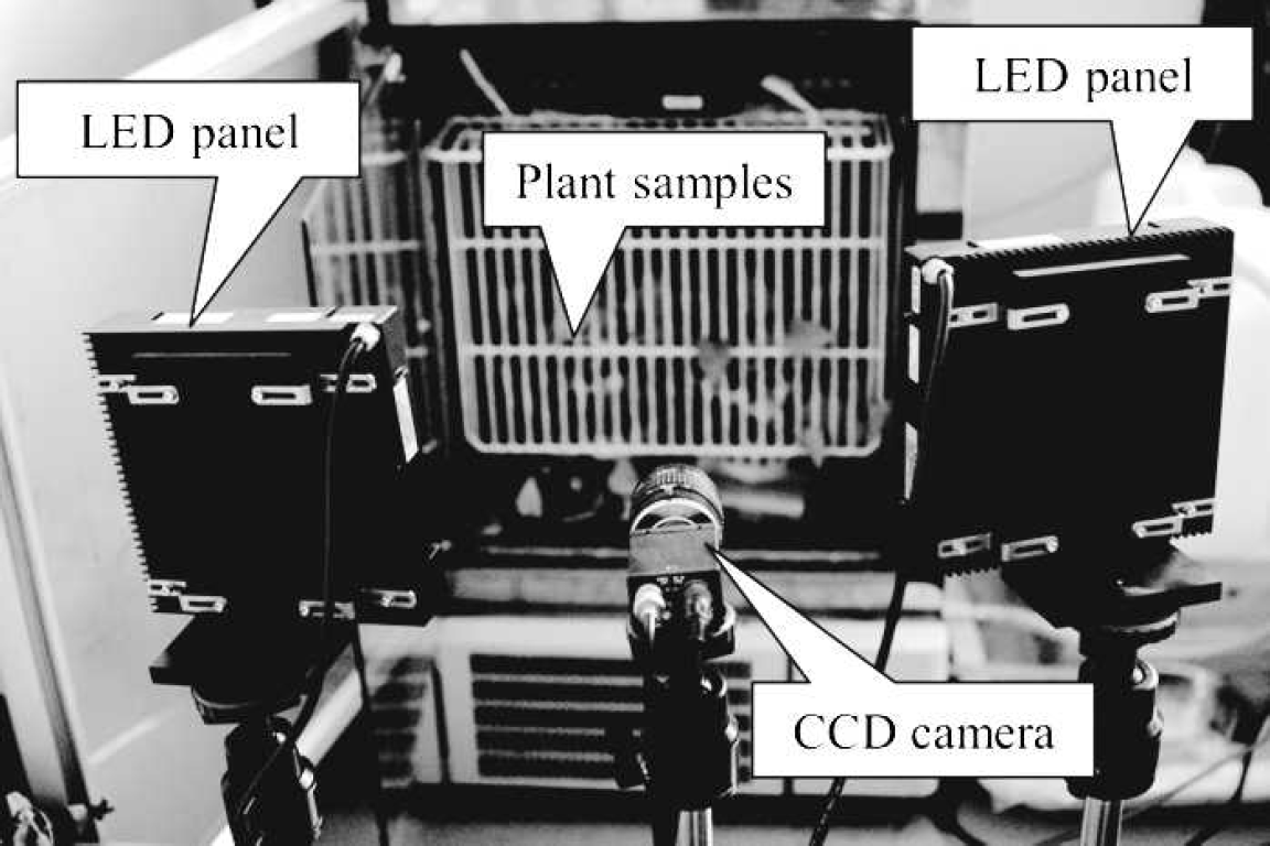
Outline of experimental device.

Four hydroponically cultivated Epipremnum aureum plants were used in this study. We selected six leaves from two potted E. aureum for fluorescence image acquisition and fixed them on a steel fence. The same experiments were repeated twice. First experiment was labeled as Ex-A and is applied for the calculation of principle component (PC) loading vector. Second experiment was labeled as Ex-B and was used as PC score images.

Image Acquisition and PCA for Time Dependency of CFI. The time after stopping water supply for one pot, that is, the time of exposure to water stress was defined as Twst. The water supply for 100 mL/day was held for another pot as a control. Images were captured 15 times from Twst = 1–17 days by once a day (days 9–11 were deficient due to the instrument error). Time-resolved CFI images were captured by a CCD video camera module (XC-ST50, SONY, Japan) at 640 × 480 pixels. The band-pass filter (maximum transparent wavelength, 730 nm; half bandwidth, 30 nm) for monitoring chlorophyll fluorescence was mounted in front of the lens. Time-resolved CFI images were captured at 3 frames/s for 20 s after starting irradiation (time after starting irradiation was defined as Tir); complete images totaled 53 frames. This three dimensional luminance brightness matrices which size is 480 × 640 × 53 is labeled as I.

Figure 2 shows the representative chlorophyll fluorescence image of E. aureum leaves. As shown in Fig. 2, the region of interest (ROI) for six leaves (from a to f) was determined manually. The size of each ROI was 900 pixels, and their average was calculated, i.e., six time dependencies of CFI were extracted from each I. Finally, 90 time dependencies of CFI were acquired from Ex-A. Time dependency was subjected to matrix X, 90 × 53 in size, to obtain PC loading vector.

OPEN IN VIEWER

Fig. 2.

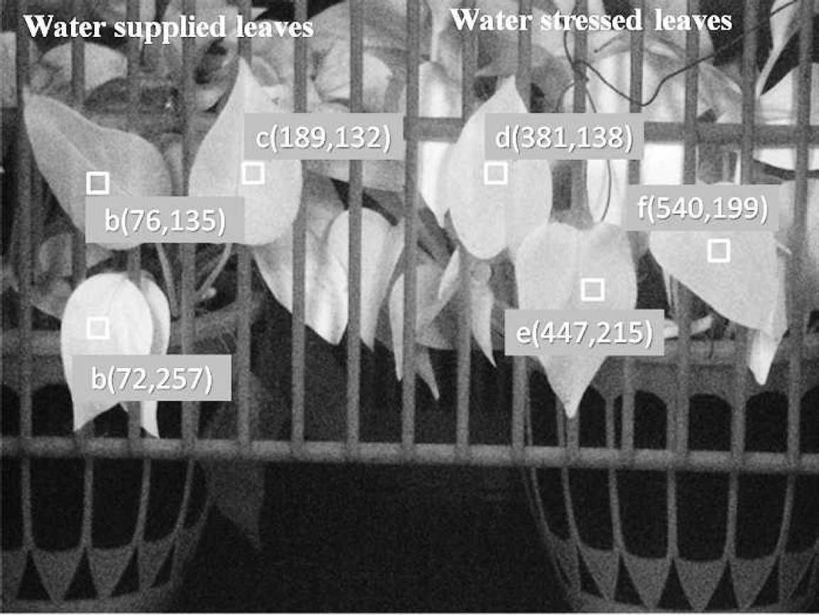
Representative chlorophyll fluorescence image of Epipremnum aureum leaves acquired at Tir = 3 s and Twst = 1 day of Ex-A. Coordinate values in the figure express the upper left pixel locations of each ROI.

For PCA, explanatory variable X is expressed as the product of the score matrix T and the transposed loading matrix P′.

X = T P ′

(1)

T = [ t 1 , t 2 , t A , ⇌ , t 53 ]

(2)

P = [ p 1 , p 2 , p A , ⇌ , p 53 ]

(3)

Note that tA and pA are the Ath score vector and loading vector of the PC, respectively. Matrix P actually contains the eigenvectors of X⁰X. In this experiment, PCA was conducted without pretreatment.

Score Image Calculation. Figure 3 depicts the outline of image processing. Score images for each matrix I of Ex-B were calculated from each I. Loading vectors calculated from matrix X of Ex-A were applied. I of Ex-B was reshaped into two-dimensional matrices RI. Their ith row was composed of 307 200 (480 × 640) elements due to the ith number matrix of I. Their jth column also was composed of 53 elements, corresponding to the variation of luminance brightness at a specific pixel of the CCD camera over time of irradiation. Then, PC score T for I is subjected as follows:

OPEN IN VIEWER

Fig. 3.

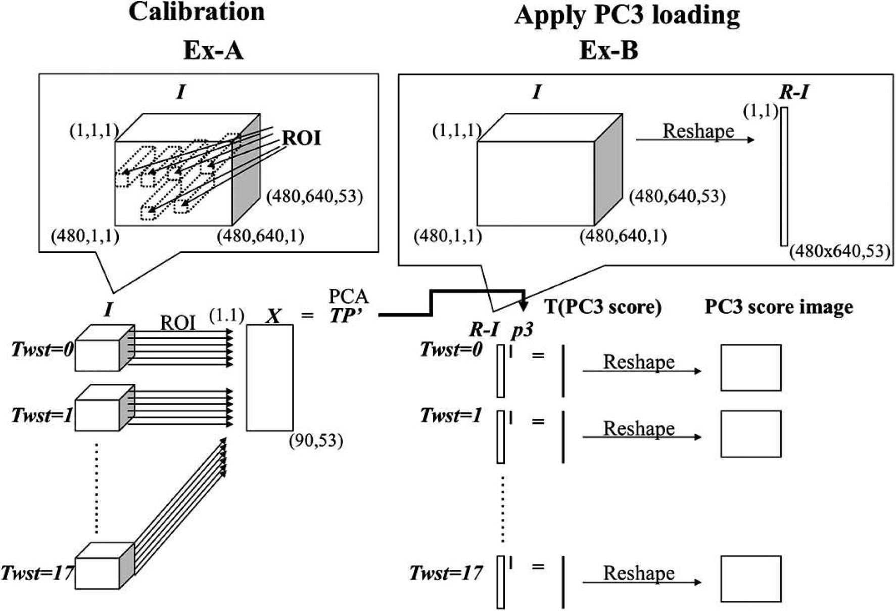
Outline of image analysis for Ex-A and Ex-B.

T = ( R I ) p

(4)

where p is loading vector calculated from X of Ex-A.

RESULTS

Time Dependency of CFI and Loadings of Ex-A. Figure 4 shows the averaged time profile of CFI at each leaf ROI. The variations in representative intensity of luminance brightness of chlorophyll fluorescence with Tir, defined as the average of 900 pixels at the center of each leaf, there are noticeable peaks around Tir = 3 s due to maximum closure of PSII reaction centers. ¹⁷ The time profile of CFI for stressed leaves dramatically changed (Fig. 4).

OPEN IN VIEWER

Fig. 4.

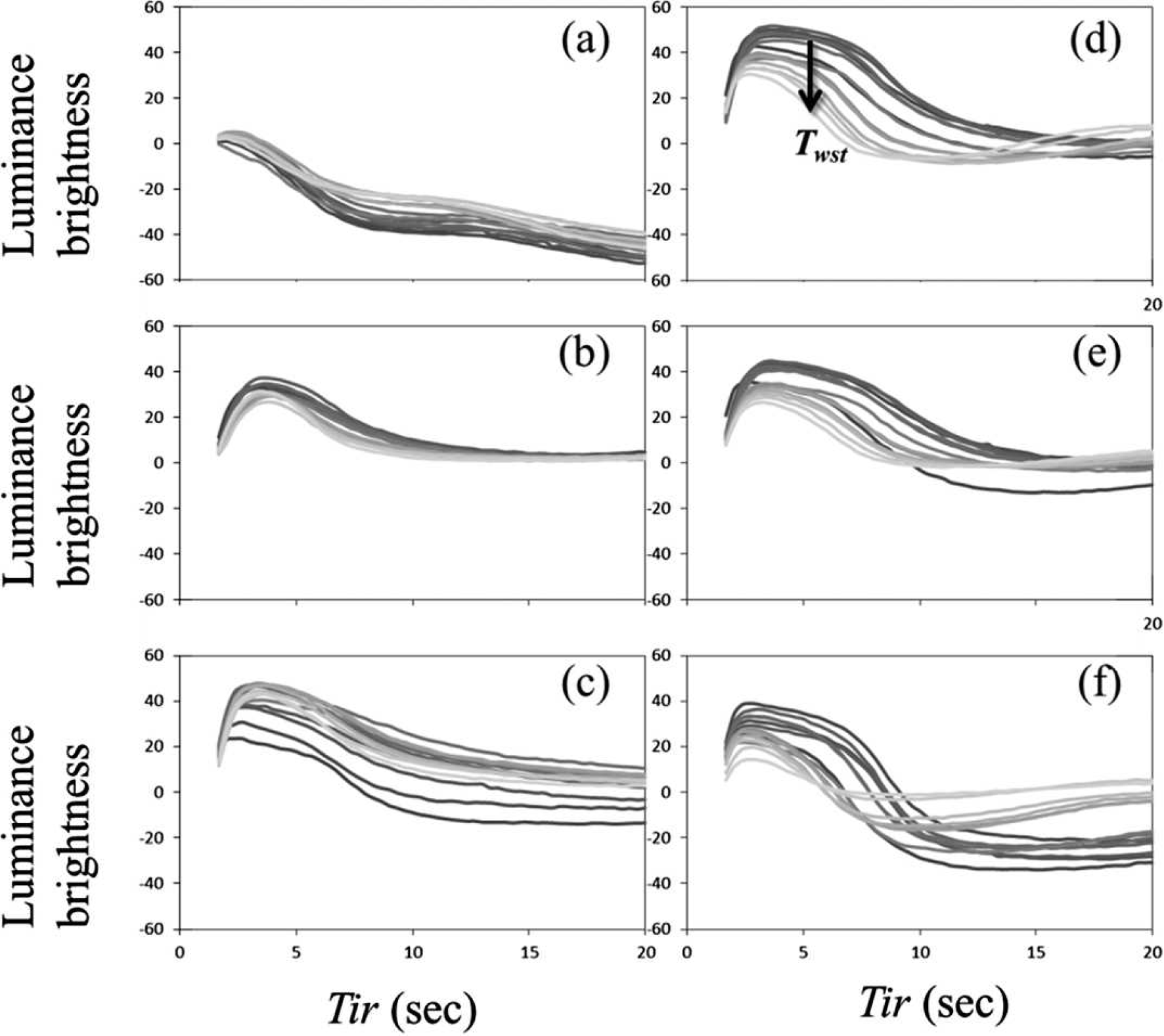
Averaged time profile of CFI at each ROI for control leaves (a–c) and stressed leaves (d-f). The gray level of each line represents Twst; the darkest line is Twst = 1 day and the lightest line is Twst = 17 days.

There are several differences between control and stressed leaves (Fig. 4). After the maximum florescence intensity at Tir = 3 s, fluorescence intensity moderately decreases until Tir = 7–15 s. As the Twst increases (stressed), the decrement occurs faster, so that the fluorescence intensity of stressed leaves at Tir = 6–8 s is lower than that of control leaves. Another difference could be observed at Tir = 10–20 s. Fluorescence intensity of stressed leaves at Tir = 10–20 s slightly increases, i.e., fluorescence intensity of stressed leaves at Tir = 20 s is higher than that of the control. The Tir at maximum fluorescence intensity (approximately Tir = 3 s) of stressed leaves slightly shifts to the shorter time as Twst increases. The peak shift causes the increase of fluorescence intensity at Tir = 2.5 s.

The time profile of CFI for control leaves a and b did not change greatly during measurement. However for leaf c, fluorescence intensity increased at the beginning of Twst, which seems baseline drift and completely differs from that of stressed leaves. However, such drift phenomena could not be clarified due to unexpected leaf movement, as the angle between the camera and the leaf surface changed.

Figure 5 shows the PC1 to PC4 loading vectors calculated from Ex-A. As described above, the differences in fluorescence intensity between stressed and control leaves appear at Tir = 2.5 s, 6–8 s, and 20 s, respectively. Fluorescence intensity at Tir = 2.5 and 20 s increases for water stress and that at Tir = 6–8 s decreases for water stress. PC3 is better for expressing the differences between stressed and control leaves (Fig. 5); PC3 loading at Tir = 2.5 s and 20 s shows negative values and Tir = 7.5 s shows a positive peak. These peaks could enhance the difference between stressed and control leaves. Every PC scores were compared, and then we used the PC3 to detect water stress.

OPEN IN VIEWER

Fig. 5.

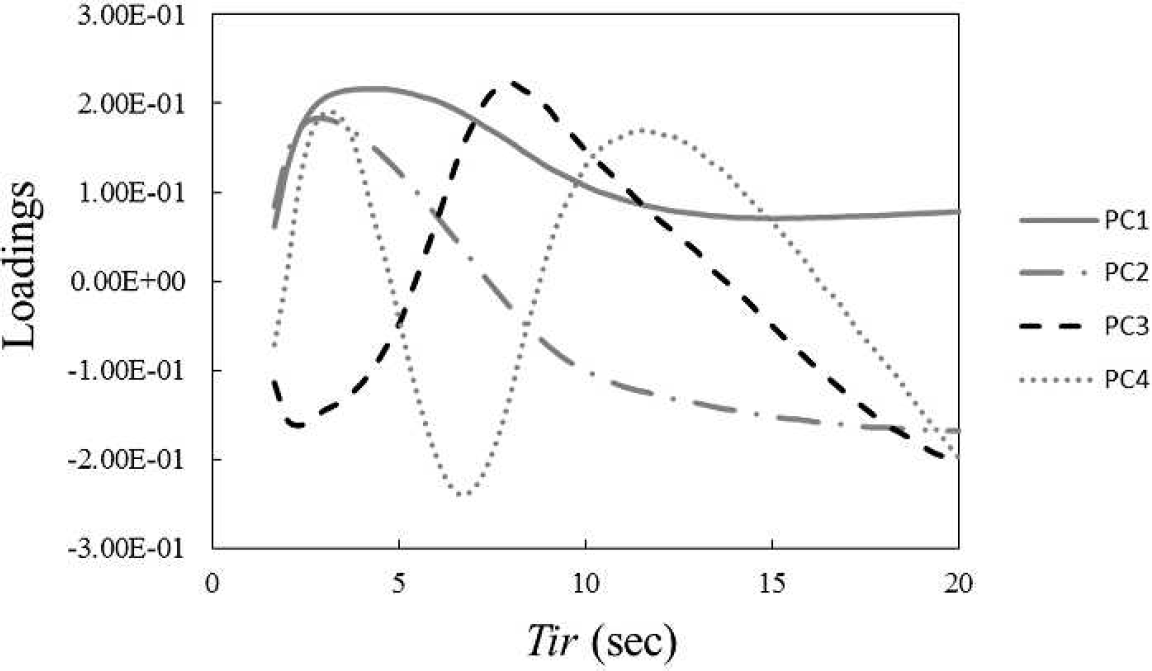
PC loading vectors of CFI. PC3 loading accurately described the CFI of stressed leaves.

PC3 Score of Ex-A and B. Figure 6 shows the time dependency of averaged PC3 scores for Twst for each ROI of Ex-A. The PC3 scores at the ROI of leaves a–c (see Fig. 2, the control leaves) remained at almost a constant level. However, PC3 scores of stressed leaves d–f increased rapidly at the beginning of five days and then daily decreased. From the observation of the PC3 loading vector, score value is mainly caused by the changes in fluorescence intensity at Tir = 2.5 s, 7.5 s, and 20 s. As discussed in the preceding section, fluorescence intensity at Tir = 2.5 s and 20 s increases and that at Tir = 6–8 s decreases as Twst increases (see Fig. 4). Furthermore, decrement of fluorescence intensity at Tir = 7.5 s occurs as the increases of Twst. Conversely, fluorescence intensity at Tir = 20 s was constant at the beginning of Twst, and the increment occurs only at later stages of Twst. Thus, the daily decrement of PC3 scores for stressed leaves after Twst = 5 days was mainly due to the increment of fluorescence intensity at Tir = 20 s. For leaf f, the PC3 score rapidly increased after Twst = 14 days. This increase is due to the dynamic increment of fluorescence intensity at Tir = 20 s, after Twst = 14 days (see Fig. 4f). The reason why only the PC3 score for leaf f changed drastically is not clear; however, this leaf seems to experience stronger stress than leaves d and e.

OPEN IN VIEWER

Fig. 6.

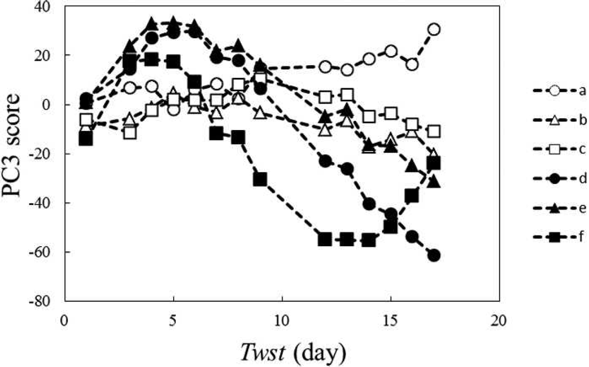
Time dependency of PC3 score of each ROI. Plots show water-supplied leaves (a–c) and stressed leaves (d–f).

Then, PC3 loading vector of calibration was applied to Ex-B. Figure 7 shows score image of Ex-B. To clarify the difference between control and stressed leaves, score images were binarized at the threshold of −4. These images are calculated from matrices I of Ex-B, and the PC3 vector was calculated from Ex-A. At Twst = 12 days and 17 days, stressed leaves could be detected clearly. As shown in Fig. 6, PC3 scores of stressed leaves first increase and then decrease. The water stress condition of leaves could be estimated by tracing the changes of PC3 scores.

OPEN IN VIEWER

Fig. 7.

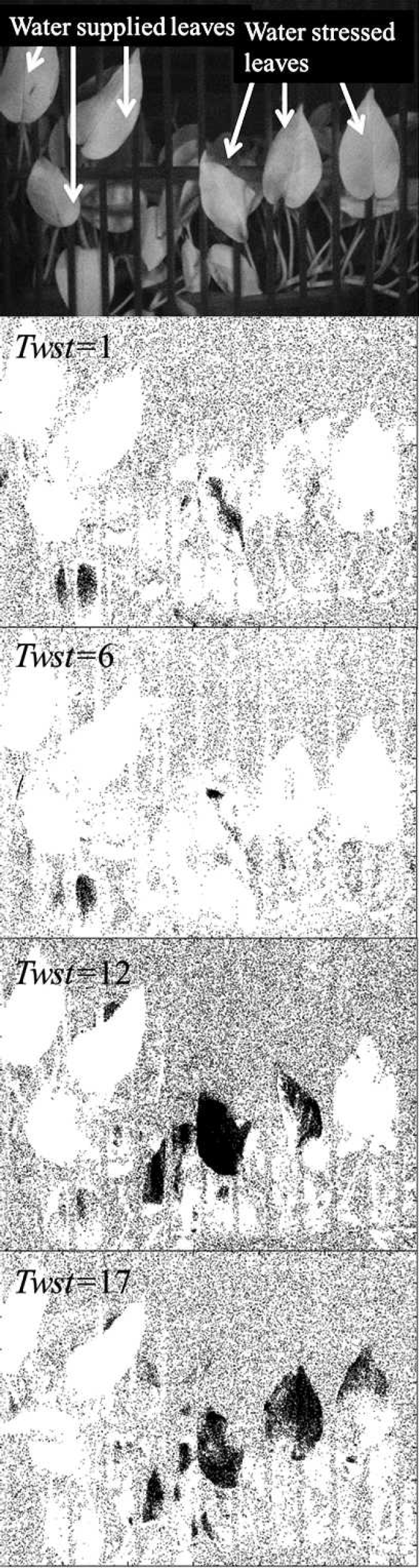
PC3 score image for Ex-B.

DISCUSSION

The PC3 score of each of the leaves examined in this study was somewhat different, even at the initiation of the experiment (see Fig. 6). This difference was not induced by water stress but was due to individual variability in CFI affected by various factors, such as another type of environmental stress or the concentration of chlorophyll within the leaf (see Fig. 3). Thus, it was difficult to detect the water stress condition at the initial stage. However, in a longer-term water-stressed condition, PC3 scores of the stressed leaves were higher than that of the control. These results allowed us to conclude that the score image is useful to detect long-term water-stressed leaves. Moreover, the PC3 score of control leaves showed a constant value, whereas the score of stressed leaves showed characteristic variation with the time of exposure to water stress. This result suggests that continuous monitoring of PC3 score of CFI could be applied for the routine monitoring of water-stressed status.

CONCLUSIONS

Time-resolved principal component imaging analysis was performed to evaluate the water stress condition of plant leaves. We examined the time dependency of CFI and applied PCA loading to distinguish stressed leaves from control (non-stressed) leaves. PC3 score images made it possible to reliably compare the differences between control and stressed leaves. PC3 score images could detect long-term water-stressed leaves. In this experiment, the difference between control and stressed leaves was due only to water supply conditions, and any other parameters, such as temperature, humidity, and irradiation, were stable. However, these parameters should effect CFI. When this technique is applied to monitor the water-stress condition of plants grown outside the laboratory, various parameters should be considered. For the application of this technique, additional experiments are required to distinguish the various kinds of stress. This technique could be used for in vivo stress monitoring of plants.