Sequentially Shifted Excitation Raman Spectroscopy: Novel Algorithm and Instrumentation for Fluorescence-Free Raman Spectroscopy in Spectral Space

Abstract

A novel Raman spectrometer is presented in a handheld format. The spectrometer utilizes a temperature-controlled, distributed Bragg reflector diode laser, which allows the instrument to operate in a sequentially shifted excitation mode to eliminate fluorescence backgrounds, fixed pattern noise, and room lights, while keeping the Raman data in true spectral space. The cost-efficient design of the instrument allows rapid acquisition of shifted excitation data with a shift time penalty of less than 2 s. The Raman data are extracted from the shifted excitation spectra using a novel algorithm that is typically three orders of magnitude faster than conventional shifted-excitation algorithms operating in spectral space. The superiority of the instrument and algorithm in terms of background removal and signal-to-noise ratio is demonstrated by comparison to FT-Raman, standard deviation spectra, shifted excitation Raman difference spectroscopy (SERDS), and conventional multiple-shift excitation methods.

Keywords

Shifted excitation Raman difference spectroscopy (SERDS)Raman Handheld Fluorescence-free Tunable excitation source Raman Instrumentation

INTRODUCTION

Although Raman spectroscopy is a powerful analytical method for molecular analysis, Raman spectra are often plagued with intense fluorescence backgrounds resulting from impurities or from the population of a sample's excited state(s). The use of long wavelength lasers such as the 1064 nm Nd:YAG laser commonly used for FT-Raman spectroscopy results in a significant reduction in fluorescence backgrounds.^1,2 However, since the Raman scattering is inversely proportional to λ⁴ for the excitation laser, it also results in less Raman signal and thus often requires the use of longer acquisition times and higher laser powers, which can often lead to sample burning.³ In addition, FT-Raman instruments are typically large and expensive with integral interferometers, which are sensitive to mechanical vibration. For these reasons FT-Raman spectroscopy does not easily lend itself to applications involving process control or remote deployment. Alternatively, dispersive Stokes Raman instruments using CCD detection with solid-state laser excitation provide a robust no-moving-parts option. However, the use of shorter wavelength excitation required for silicon CCD detection in these systems results in significantly more fluorescence.⁴

It is well known that fluorescence is a function of many external parameters including, but not limited to, sample concentration, temperature, pH, concentration of dissolved O₂, and pressure. In addition, the shape of fluorescence interference can vary dramatically (ascending background, descending background, single broad peak, and multiple sharp peaks as in the case of heavy metal ions). Fluorescence can arise not only from the sample, but also from impurities, the sample matrix, and the sample container. When taken together, this varied nature of the fluorescence background is difficult to correct for. For this reason, several methods have been developed to extract the Raman information from interfering backgrounds.

In general, these methods can be separated into four categories: algorithm-based baseline correction methods,^5–12 sampling optics and geometries,^13–15 time gating methods,^16–21 and shifted excitation methods.^22–41 The varied nature of fluorescence backgrounds has resulted in limited success for the first three methods; however, shifted excitation methods are gaining widespread use due to their successful application for any sample. In the most simplistic implementation, only two laser wavelengths are used for excitation. In this case, the only way to extract the Raman data is to take a difference of the two spectra, and hence the technique is often referred to as SERDS (shifted excitation Raman difference spectroscopy).^{25–33,40–42} The result of SERDS is spectral data in the derivative form. More recently, it has been demonstrated that by using external-grating tuned lasers in constant sweep mode, the signal-to-noise (S/N) of the Raman derivative signal can be significantly enhanced due to the presence of more than two excitation wavelengths.^30–34,42 Despite the impressive results, the true Raman spectra are not generated, and as with SERDS, there is significant difficultly in reconstructing the Raman spectra from the derivative data. In addition, the instrumentation is large and expensive, thus limiting some of the main advantages of dispersive Raman spectroscopy. Perhaps more intriguing is the recent work of Willet and colleagues in which a series of diode lasers at closely spaced wavelengths are used for the acquisition of shifted Raman spectra. The setup allows the researchers to extract the spectral data in true Raman space using an iterative expectation-maximization (EM) algorithm (Lucy-Richardson algorithm) based on a shift-matrix operator. This is the first example of the extraction of Raman data regardless of the complexity or nature of the fluorescence background (i.e., a universal approach). Despite the promise of the method, the instrumentation remains complex, and it can be anticipated that reproducing the series of selected wavelength lasers would not be possible for multiple instruments. In addition, the processing of the data using the shift-matrix operator requires tens of billions of double-precision calculations, so processing time often requires several minutes for high background spectra. In the current work we present a new algorithm and instrumentation that allow the acquisition of fluorescence-free Raman spectra. We demonstrate that the practical nature of the instrumentation allows for implementation of shifted excitation Raman spectroscopy even in a low cost handheld design. A new algorithm is presented here that allows for true Raman signal extraction identical in spectral performance to existing EM algorithms, but is three orders of magnitude faster. This method relies on sequentially shifted excitation (SSE) using a single temperature-controlled distributed Bragg reflector diode laser.

EXPERIMENTAL SECTION

Instrument Design and Operation. The design of the SSE Raman instrument is shown in Fig. 1. The excitation source (Fig. 1A) is a distributed Bragg reflector (DBR) GaAs diode laser mounted on a Peltier cooler and contained within a custom TO-8 package. The DBR laser emits single-mode 785 nm radiation at an operational temperature of 25 °C. The Bragg grating of the DBR laser is a periodic structure etched into the GaAs substrate at the rear facet of the diode cavity. Hence the cavity and the grating consist of a monolithic structure. The emission wavelength of the laser at a given temperature is equal to

Fig. 1.

The SSE Raman spectrometer is composed of (A) a 785 nm DBR GaAs diode laser, (B) collimating asphere, (C) focusing/collimating asphere, (D) laser bandpass filter, (E) dichroic beam splitter, (F) long-pass filter, (G) focusing doublet achromat, (H) 40 micrometer rectangular slit, (I) collimating doublet achromat, (J) long-pass filter, (K) 1500 groove/mm volume holographic transmission grating, (L) focusing doublet achromat, (M) CCD detector, (N) microprocessor control board, and (O) thermoelectric control/laser diode driver control board.

λ = 785 n m + 0.074 \frac{n m}{° C}

(1)

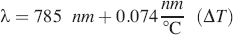
where ΔT is the set-point temperature of the thermoelectric cooler (TEC) minus 25 °C. The feedback from the Bragg grating stabilizes the modal structure of the laser so that when the laser is operated at a constant current, a range of ΔT exceeding 15 °C is obtainable without a change in the single-mode modal structure of the laser output (i.e., no mode hops occur). Although the Bragg grating stabilizes the laser, it is possible to encounter regions of wavelength instability at a given temperature and current. For this reason, the laser is operated in a constant current mode, which will give a desired optical output. In some cases, it may be necessary to adjust this current set point in order to obtain a large tunable temperature range. Our experience has shown that such adjustments do not affect the optical output power of the laser by more than 15%. For a particular spectrometer, once the set-point current has been determined, it is not changed.

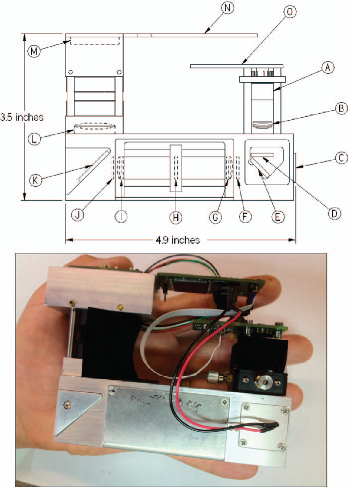
We have evaluated five different DBR lasers, all of which have demonstrated this characteristic (consistent with current-voltage curves for each device supplied by Photodigm, Dallas, Texas). For the current work, a sample-incident optical power output of 50 mW was selected, and the laser was run in constant current mode (100 mA) by using a fixed resistance on the laser diode constant current supply (Fig. 1O). The TEC controller is capable of 0.01 °C precision. This provided a stable mode, hop-free temperature range from 16 °C to 34 °C. A typical measurement consists of collecting Raman spectra at DBR laser temperatures of 20, 23, 26, and 29 °C (i.e., four sequential excitations that are evenly spaced in temperature. This yields excitation wavelengths of 784.630, 784.852, 785.074, and 785.296 nm, respectively, while running in constant current mode at 100 mA. This gives a constant excitation shift of 0.222 nm. When converted to cm⁻¹, this gives a separation of approximately 3.60 cm⁻¹ between the different excitations (approximate since the cm⁻¹ scale is linear to 0.01 cm⁻¹ over such a small change in wavelength). Due to the presence of the DBR grating and the use of optics with antireflection coatings, we have not been able to observe any changes in laser quality due to back-reflections into the diode cavity resulting from sample placement. For this reason an optical isolator in front of the diode laser was omitted in the current design.

The DBR diode laser (Fig. 1A) beam is collimated with a 0.55 N.A. asphere (Fig. 1B) and filtered with a bandpass filter (Fig. 1D). A dichromic beam splitter (Fig. 1E) directs the laser beam through a focusing 0.50 N.A. asphere (Fig. 1C) onto the sample. The asphere-collected Raman scatter is passed through the beam splitter and a high-pass filter (Fig. 1F) and is then focused by a 12.7 mm diameter doublet achromat of focal length 32 mm (Fig. 1G) onto a 1 mm × 50 μm slit (Fig. 1H). An identical achromat (Fig. 1I) is used to collimate the light passing through the slit. The collimated light is passed through a second high-pass filter (Fig. 1J) and diffracted using a volume holographic transmission grating (1500 gr/mm) mounted at −45° to the optical axis (Fig. 1K). The diffracted light is focused onto an uncooled back-thinned CCD detector (Hamamatsu model S11071–1006, Fig. 1M) using a 45 mm focal length doublet achromat (Fig. 1L, 25.4 mm diameter to account for the anamorphic magnification of the grating). The design provides a spectral resolution of approximately 10 cm⁻¹. A microcontroller board (Fig. 1N) is used to control both the TEC and the CCD data acquisition and to upload collected raw spectra to a processing CPU over a USB 2.0 connection. The TEC and the constant current laser diode driver reside on a separate board (Fig. 1O).

Although the instrument can be operated in a variety of manners, the use of a microcontroller allows programming of a set sequence of events, which minimizes acquisition time and electrical power consumption. For the current work these steps included: (1) turning on TEC, (2) cooling the laser to a starting temperature of 20 °C, (3) turning on the laser, (4) resetting the CCD and collecting spectrum, (5) turning off the laser, (6) heating the laser to the next temperature and uploading data, (7) repeating steps 3–6 until final spectrum is collected, and (8) turning off TEC. For this sequence, the most time-consuming steps are 2 and 4. Due to the small mass of the diode laser, the time to cool the laser (when room temperature is <30 °C) is less than 1 s. The time required to heat the laser to the next temperature is 300 ms for temperature steps of 6 °C or less. The time to upload the data is 28 ms and thus has no time penalty since it occurs during the TEC heating period. The time required to turn the laser on and off is less than 1 μs. Thus the total acquisition time for a four-temperature experiment is equal to the total integration times of the spectra plus <2 s. It should be noted that although there is an increase in the laser temperature during the “heating” period, the laser is not actively heated. When the set-point temperature of the laser is increased, the effect on the feedback loop of the thermoelectric controller is to decrease the active cooling to the laser, which results in a rapid temperature rise until the set-point temperature is reached. At this point, the TEC resumes active cooling (albeit at a lower drive current from the TEC).

Theoretical Aspects of Shifted Excitation Raman Data Processing Fluorescence-removal techniques that involve changing the excitation laser wavelength during Raman spectral acquisition all rely on a common concept: The location of Raman intensities in spectral space changes with excitation wavelength, while unwanted spectral intensities corresponding to fluorescence, stray light, fixed pattern detector noise, etc., remain unchanged in spectral space. The difference in the various methods to date occurs in how the spectra are acquired and how the Raman data are extracted. The simplest extraction method is taking a difference between two sets of excitation data (SERDS) and requires only excitation at two distinct wavelengths. This type of method has two distinct disadvantages: random noise in two measurements is increased during subtraction, and the result is a derivative spectrum instead of a true Raman spectrum in spectral space. With the addition of more than two excitation wavelengths, however, multivariate solutions can be used to extract the Raman intensities while minimizing noise. In such cases, the Raman spectra acquired at each unique laser excitation can be described by a matrix R:

R = (\begin{array}{l} r_{0, 0} & \dots & r_{0, n} \\ ⋮ & ⋱ & ⋮ \\ r_{k, 0} & \dots & r_{k, n} \end{array})

(2)

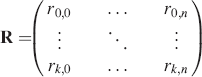
where each row corresponds to the Raman spectrum acquired with k laser excitation (total of K excitations), and n is the spectral index and each spectrum has a spectral length of N. Using conventional matrix decomposition such as singular value decomposition (SVD), R can be related to a loadings matrix L:

R = T L^{T}

(3)

where L^T is the transpose of the loadings matrix and where there are K rows in L and each row corresponds to a principal component (loading vector) that describes orthogonal variance in R. The scores matrix T relates how much of each principal component is required to reconstruct each spectrum in R. A characteristic of the loading matrix is that the principal components are sorted in descending order of variance. Since the principal variation of R is the change in excitation laser wavelengths when collecting the data, and since this principally affects only the Raman signal, the first principal component describes the variation in the Raman signal as the excitation laser wavelengths are changed and is observed as a pseudo-derivative Raman spectrum. The spectral components that are independent of small changes in excitation wavelength (e.g., fluorescence) as well as a portion of the random noise are described by the higher principal components. This method is similar to SERDS, but has the added advantage of reducing spectral noise as opposed to increasing it. For both methods, however, generating the original Raman spectrum without a background is often difficult or impossible for many samples.

An alternative method for solving for the Raman spectrum when using multiple excitations involves relating the desired outcome (separated Raman spectrum and fluorescence spectrum) to the collected data (R) using an operator matrix H:

H S = R

(4)

where S is a 1 × 2N matrix containing a column vector of spectral events that are independent of small changes in excitation wavelength such as fluorescence (S^F) and a column vector corresponding to the true Raman signal (S^R):

S = (\begin{array}{l} S^{F} \\ S^{R} \end{array}) = (\begin{array}{l} (\begin{array}{l} s_{0}^{F} \\ ⋮ \\ s_{0}^{R} \end{array}) \\ (\begin{array}{l} s_{0}^{R} \\ ⋮ \\ s_{n}^{R} \end{array}) \end{array})

(5)

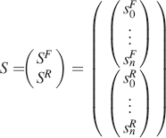
where both the fluorescent spectrum (S^F) and the Raman spectrum (S^R) consists of N spectral positions. The spectral data matrix (R) is rewritten as a concatenated column vector of spectra:

R = (\begin{array}{l} R_{0} \\ ⋮ \\ R_{k} \end{array}) = (\begin{array}{l} (\begin{array}{l} r_{0, 0} \\ ⋮ \\ r_{0, n} \end{array}) \\ (\begin{array}{l} r_{k, 0} \\ ⋮ \\ r_{k, n} \end{array}) \end{array})

(6)

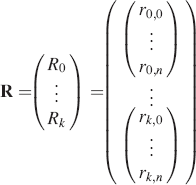
where each spectrum has N spectral positions of intensity r_k;n at each spectral position, and there are a total number of spectra corresponding to the number of excitations (K). The operator matrix H consists of two columns of N × N square submatrices:

H = (\begin{array}{l} H_{0}^{F} & H_{0}^{R} \\ H_{1}^{F} & H_{1}^{R} \\ H_{2}^{F} & H_{2}^{R} \\ ⋮ & ⋮ \\ H_{k}^{F} & H_{k}^{R} \end{array})

(7)

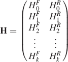
where the first column corresponds to submatrices that describe the spectral position of fluorescence intensity (H_k^F) at each excitation (k), and the second column corresponds to submatrices that describe the spectral position of Raman intensity at each excitation (H_k^R). Due to the sparse nature of the operator matrix, it is not possible to explicitly solve Eq. 4 for S. However, an iterative approximation algorithm such as a Lucy-Richardson formula has been invoked and requires only a reasonable initial estimate of S^R and S^F to be provided. For example, selecting the maximum spectral intensity from each k spectrum at each spectral position n will maximize Raman contributions yielding an initial Raman estimate (S^R₀). Likewise, selecting the minimum spectral intensity from each k spectrum at each spectral position n will minimize Raman contributions yielding an initial fluorescence estimate (S₀ ^F ). This iterative approach using an operator matrix is shown in Eq. 8:

S_{i + 1} = s_{i} \times (H^{T} (R \div H S_{i}))

(8)

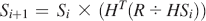
where multiplication and division operators are carried out element-wise and i is the iteration number (H, S, and R remain defined as in the previous three equations). Using this approach, McCain and co-workers have reported resolution of background-free Raman spectra using 100 iterations or less when the method is combined with denoising approaches. However, as can be observed, the large size of the operator matrix (2N × kN) results in an extensive number of calculations. We have experienced that using this approach on a conventional desktop computer (1.8 GHz single core x86 processor running Windows XP) typically requires over 2 min to carry out 500 iterations when N = 1024 and k = 4 (over 25 billion calculations, each requiring double precision). Indeed, the numerically intensive nature of this approach is the reason behind the inclusion of denoising steps to minimize the iteration number. Without a denoising step, convergence does not often occur before 1000 iterations.

Since each row of the submatrices of the operator matrix (Eq. 8) consists of a single unity value with the remaining elements being zero, the operator matrix is sparse. As one would expect since the fluorescence spectrum is not expected to change with excitation wavelength, for the first column of submatrices, every submatrix is the N × N identity matrix. Also, the first submatrix in the second column of submatrices is the N × N identity matrix, as expected since k = 0 and the laser excitation has not changed yet. Consideration of the facts that multiplication by the identity does not cause change, and considering that anything times zero is equal to zero, leads to the conclusion that there exists a much simpler and more efficient method. Our approach is to use a weighting vector, ŵ _i , which is calculated with each iteration, i :

{\hat{w}}_{i} \sum_{k = 0}^{K - 1} R_{k, n} \div (S_{i, n}^{F} + S_{i, n - k}^{R})

(9)

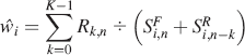
where the division and addition operators are carried out element-wise. Then for each iteration i , the fluorescence spectrum is then calculated as

S_{i + 1}^{F} = S_{i}^{F} \times {\hat{w}}_{i}

(10)

and the Raman spectrum is calculated as

S_{i + 1}^{R} = S_{i}^{R} \times {\hat{w}}_{i}

(11)

Significantly, the number of calculations using this approach is proportional to k × N per iteration, while that of Eq. 8 is proportional to k × N² per iteration. For a spectral acquisition with 1000 spectral points (typical of CCD detection), this results in a decrease by three orders of magnitude in the number of calculations, resulting in total processing times of a fraction of a second using a conventional desktop computer (1.8 GHz single core x86 processor running Windows XP). When presented with identical spectra, both algorithms yield identical results for S . In addition, the simple nature of Eq. 9–11 allows implementation with only a few lines of simple code in common computer languages such as C as a result of the elimination of the operator matrix. Elimination of H and its transpose also results in a massive reduction in memory requirements for the CPU. Significantly, a part of the simplicity of the approach lies in the use of a fixed change in wavelength (excitation shift) between the utilized excitations. Use of varying excitation shifts would require the incorporation of a vector that indexes each of the shifts for each k calculation.

As presented, this new approach (Eq. 9–11) and the previous method (Eq. 8) both require that a spectral shift corresponds to the minimum difference in wavenumbers between the spectral data points. With the current method, this is possible by selecting the appropriate laser temperatures. However, if a series of different lasers are used with nonconstant wavelength spacing, then the data must be splined so that the operator matrix indices can accommodate the varying shifts. The resulting loss in symmetry of the operator matrix not only complicates both algorithms, it also results in the requirement that the algorithm be specifically tailored for each instrument that is produced. In addition, splining the data to obtain the requisite shift resolution will result in an increase in N, which further increases the processing time.

RESULTS AND DISCUSSION

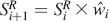
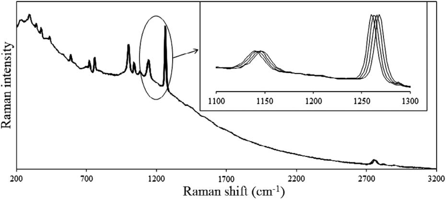
Figure 2 shows the spectral data for the acquired Raman spectrum of dimethyl glyoxime acquired at four temperatures (20, 23, 26, and 29 °C) with a 785 nm DBR laser. Although it is difficult to resolve the spectra across the full spectral range, as shown in the inset, the change in laser temperature results in a shift of about 3.6 cm⁻¹ for each of the spectra, and the underlying background remains unchanged. In Fig. 3 the result of demodulating this data using Eq. 9 and 11 is shown along with the FT-Raman spectrum acquired using a 1064 nm laser. As can be observed, the two methods yield comparable results with both resulting in an absence of the fluorescence background. In the case of the FT-Raman spectrum, the absence of the fluorescence background is due to the long wavelength of the 1064 nm excitation laser. Although the results are comparable, the two experiments were carried out under dramatically different laser powers (800 mW for the FT-Raman and 50 mW for the SSE experiment). In both cases, the excitation laser was focused. In addition, the total acquisition time for the FT-Raman spectrum was dramatically longer (120 s) compared to that of the SSE experiment (four spectra each integrated for 800 ms). The slightly higher resolution of the FT-Raman spectrum is due to its acquisition at 8 cm⁻¹ resolution. Since neither instrument was corrected for spectral intensity throughput, the relative intensities of the peaks are not identical. This is particularly true when comparing the fingerprint region (e.g., below 1800 cm⁻¹) to the CH-stretching region (e.g., above 2700 cm⁻¹). For the dispersive instrument, the silicon CCD detector has a minimum quantum efficiency for the CH-stretching spectral range (greater than 1020 nm), while for the FT-Raman spectrum, this range corresponds to the maximum quantum efficiency of the InGaAs detector used.

Fig. 2.

Raman spectrum of dimethyl glyoxime acquired at four laser temperatures (20, 23, 26, and 29 °C) using a 785 nm DBR laser with an integration time of 0.8 s for each spectrum and a laser power of 50 mW. The change in laser temperature results in a shift of 3.60 cm⁻¹ for each of the Raman spectra while the underlying background remains unchanged (as shown in the inset).

Fig. 3.

(A) FT-Raman spectrum of dimethyl glyoxime acquired using a 1064 nm laser. The spectrum was acquired with an integration time of 120 s and a laser power of 800 mW. (B) SSE Raman spectrum of dimethyl glyoxime is obtained by demodulating the four spectra of dimethyl glyoxime (Fig. 2) using Eqs. 9–11. The number of iterations was 2000.

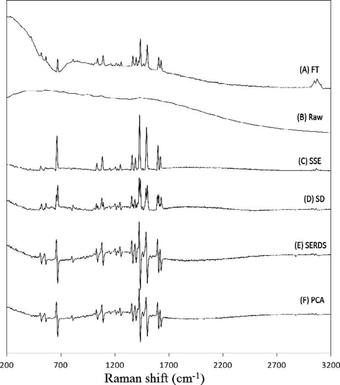
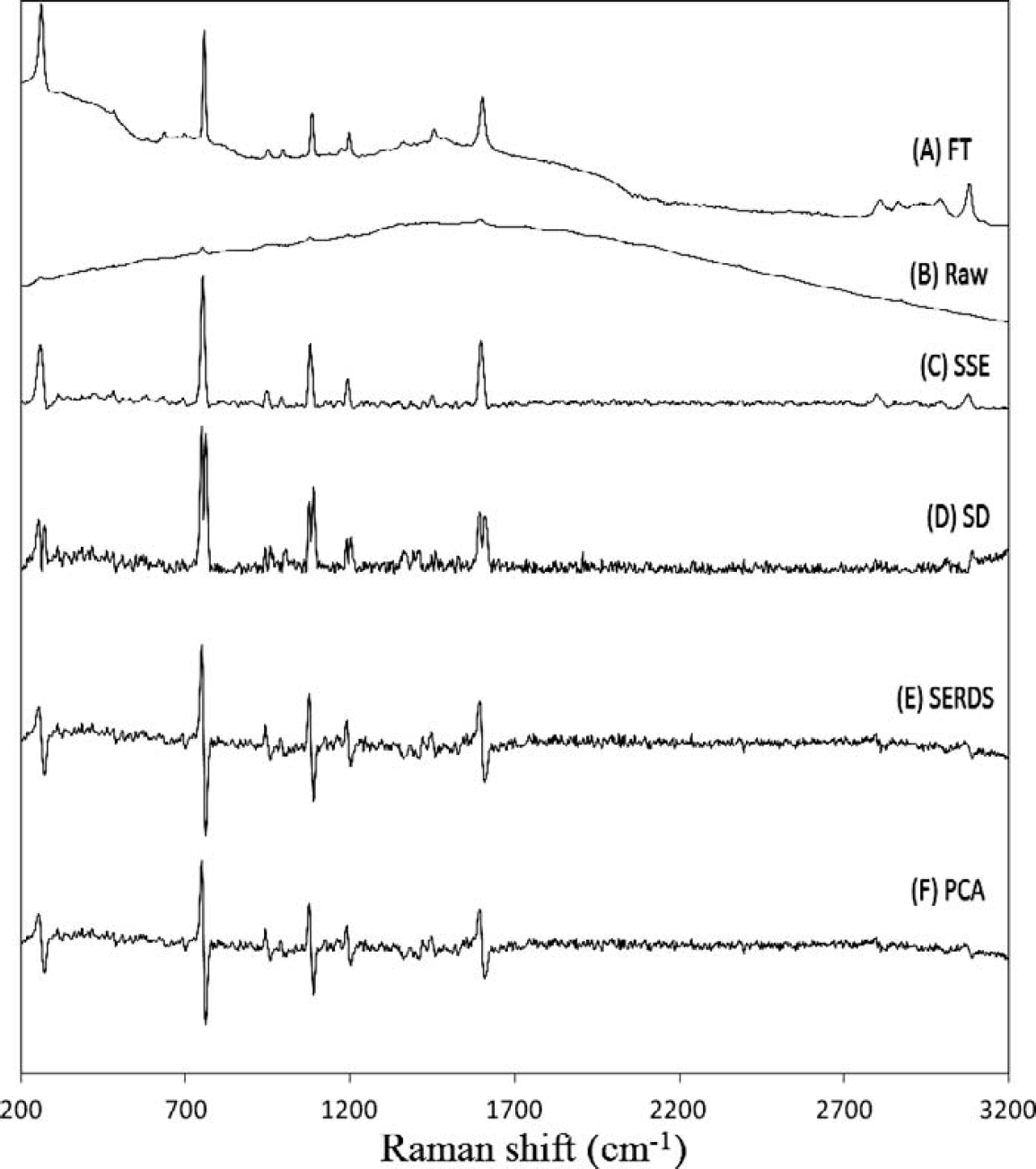
The inability of FT-Raman to eliminate all of the fluorescence for some samples is exemplified in Fig. 4A for the spectrum of acenaphthylene (cyclopentanaphthalene). For the FT-Raman, there is a significant broad undulating background even with 1064 nm excitation due to the polycyclic aromatic nature of the molecule. For the unprocessed 785 nm dispersive Raman spectrum, the fluorescence is several orders of magnitude more intense than that of the Raman scattered light. Despite this intense fluorescence, the processed four-temperature SSE data effectively eliminates the fluorescence while providing comparable S/N when compared to the FT-Raman spectrum. The same observations can be made in Fig. 5 for the spectra of 4-bromo-N,N-dimethylaniline. For these spectra, the S/N of the SSE Raman spectrum is slightly less than that of the FT-Raman spectrum. This is due to the much lower laser power and integration time for the SSE measurement.

Fig. 4.

Comparison of methods for acenaphthylene (A) FT-Raman spectrum acquired using 1064 nm laser (120 s acquisition and 800 mW). (B) Unprocessed dispersive Raman acquired using 785 nm laser at 20 °C (10 s acquisition and 50 mW). (C) Processed dispersive Raman spectra (SSE). (D) Standard deviation Raman spectrum. (E) SERDS spectrum is obtained by acquiring only two spectra (20 and 29 °C and 10 s × 2 acquisition). (F) PCA Raman spectrum. C, D, and F were all acquired at four laser temperatures (10 s × 4 acquisition and 50 mW).

Fig. 5.

Comparison of methods for 4-bromo-N, N-dimethyl-aniline (A) FT-Raman spectrum acquired using 1064 nm laser (120 s acquisition and 800 mW). (B) Unprocessed dispersive Raman acquired using 785 nm laser at 20 °C (5.2 s acquisition and 50 mW). (C) Processed dispersive Raman spectra (SSE). (D) Standard deviation Raman spectrum. (E) SERDS spectrum is obtained by acquiring only two spectra (20 and 29 °C and 5.2 s × 2 acquisition). (F) PCA Raman spectrum. C, D, and F were all acquired at four laser temperatures (5.2 s × 4 acquisition and 50 mW).

As described previously, many methods have been used to extract Raman spectra from spectral data acquired using multiple excitations. The three most successful alternative approaches are standard deviation spectra, SERDS, and PCA extraction. As a comparison, these methods are also included in Figs. 4 and 5 using the same SSE data that was used for the SSE Raman spectra (Figs. 4C and 5C). For the SERDS calculation, only two spectra are required, so the best results are displayed (this always corresponded to the largest shift between spectra, i.e., 20 °C and 29 °C, which corresponds to a total shift of 7.2 cm⁻¹). For acenaphthylene (Fig. 4), all methods give comparable S/N, but the SSE Raman in Fig. 4C results in the lowest background followed closely by the standard deviation spectrum. However, the standard deviation spectrum is difficult to interpret due to the doubling of peaks arising from the nature of the calculation. Both the SERDS and the PCA spectra result in similar yet higher levels of background. As mentioned, it is easier to observe the noise component in the dispersive spectra acquired for 4-bromo-N,N-dimethylaniline (Fig. 5). The higher S/N for the SSE Raman can easily be seen relative to SD, SERDS, and PCA. In addition, the SERDS and PCA methods still suffer from the fact that the remaining background results in a baseline which makes it difficult to retrieve the true Raman spectrum from the processed spectral data without using additional algorithmic background filtering methods.⁴²

An additional advantage of SSE over the SERDS and PCA methods lies in the fact that the SSE experiment can be carried out under a wide range of excitation conditions without impacting the resolution of the Raman spectrum result. For both SERDS and PCA methods, however, the bandwidth of the resulting derivative peaks is a function of the excitation spacing. This is demonstrated in Fig. 6 where two different excitation profiles are used. The first excitation profile consists of acquiring the spectra at 20, 23, and 26 °C, while the second excitation profile consists of acquiring spectra at 20, 26, and 32 °C. The change in the excitation wavelengths for the experiment results in a change in peak bandwidth for the PCA data but not for the SSE data. Although not shown, the effect is even more dramatic for SERDS.

Fig. 6.

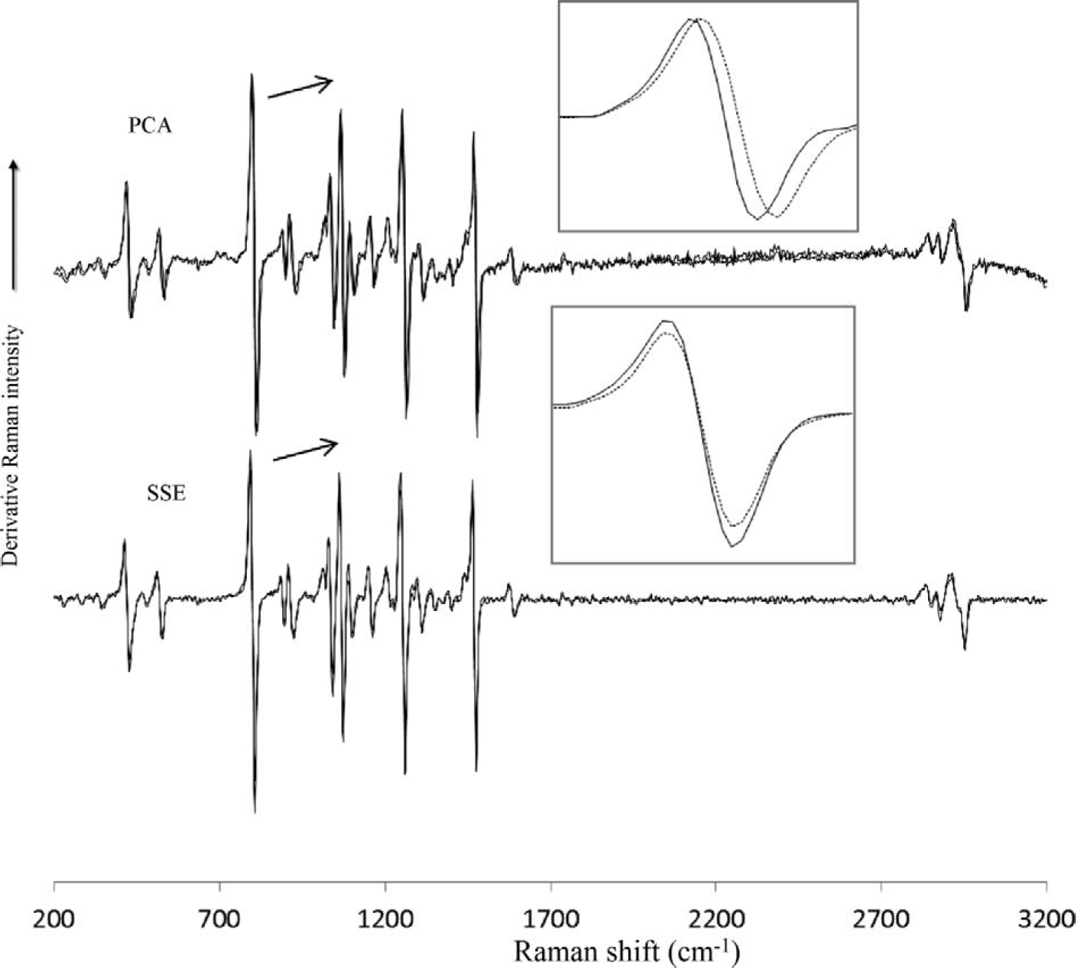
Raman spectra of tris(hydroxymethyl) aminoethane acquired at two temperature profiles; 20, 23, and 26 °C (solid line), and 20, 26, 32 °C (dotted line). The acquisition time was 1 s × 3. (A) PCA modulated Raman spectrum. (B) Derivative of SSE Raman spectrum.

The primary advantage of the SSE algorithms (Eqs. 9–11) over Eq. 8 is its execution speed since both methods utilize a Lucy-Richardson iterative method. For the current work, we have also found that using the standard deviation spectrum of the raw spectra as the initial estimate of S^R for the SSE method results in faster and more reliable convergence as opposed to using the maximum intensity of the shifted spectra at each spectral position. We have used the SSE method for more than 500 chemicals, and in each case convergence can be obtained using 2000 iterations. For samples with low levels of fluorescence or no fluorescence, this convergence is often reached with fewer iterations, although additional iterations offer no penalty in Raman quality. With samples with more dominating fluorescence, although 2000 iterations are sometimes sufficient, using iterations of 3000 or more often results in a further improvement in S/N and baseline removal. For Figs. 3 –6, all of the SSE data have been presented with 2000 iterations, and a method for autodetection of convergence has not been used. We are currently working on the development of an automatic convergence detection algorithm that will allow for user-independent selection of iteration number, which is optimized for each sample.

We would like to thank one of our reviewers for pointing out that the SERDS technique is very sensitive to types of samples. For example, Martins et al. have applied the SERDS method to study human skin and tooth and concluded that each sample presented a specific set of best parameters (grating grooving, laser power, and excitation wavelength shift) for fluorescence removal.⁴³ With regard to the SSE Raman method, we have found that the method has a universal approach in that it is not limited by the sample type, but only by the S/N ratio of the spectra and the number of iterations used in the SSE algorithm. In Fig. 7 the raw Raman spectra of a liquid diesel fuel sample are shown (Fig. 7A) along with the SSE Raman spectrum (Fig. 7B). The fluorescent background has a very high intensity at low wavenumbers and drops off significantly at high wavenumbers. Also, the Raman spectrum has regions where the Raman spectrum is very weak (300–600 cm⁻¹) as well as regions where there is significant S/N (1275–1675 cm⁻¹). In Fig. 7, an inset shows the 300–600 cm⁻¹ region with an expanded axis, and as can be seen, the shifting Raman peaks have a very low intensity compared to the fluorescence background. In addition the modulation of the fluorescence background in this region due to the response of the back-thinned CCD is quite large when compared to the weak Raman peaks. However, as shown in the SSE Raman spectrum, the algorithm is capable of extracting the peaks. The 1275–1675 cm⁻¹ region is also shown as an inset with an expanded axis, and as can be observed, the Raman peaks have significantly higher S/N. Although the Raman peaks can be observed to shift with changes in excitation wavelength, the broad underlying fluorescence remains essentially constant giving rise to pseudoisosbestic points of constant intensity in the overlaid plots. In addition, by observing the strongest peak in this region, it can be observed that there is a component that shifts with changes to the excitation wavelength (Raman intensity) as well as a relatively sharp component that does not shift with changes to the excitation wavelength, but decreases in intensity as the Raman peak shifts out from beneath it. This constant component is due to fluorescence intensity modulated by the back-thinned CCD. A comparison of this region with the SSE Raman spectrum clearly shows that only the shifted Raman peaks are retained. The superposition of the CCD response (particularly in the case of a back-thinned CCD) on an intense fluorescence signal would make it very difficult to remove the fluorescence background using just a background-removal algorithm on a single Raman spectrum since there is both a broad component as well as sharp components to the fluorescence signal. In addition, using just two spectra (as with the case of SERDS), it would also be difficult to remove the sharp components since the intensity of the sharp fluorescence component is a function of the shifting Raman peak (this is not the case for a broad fluorescence background). The peak just below 1475 cm⁻¹ exhibits similar characteristics with a very weak Raman peak shifting out from a much larger fluorescence peak. The corresponding region in the SSE Raman spectrum shows that only the small Raman peak is retained.

Fig. 7.

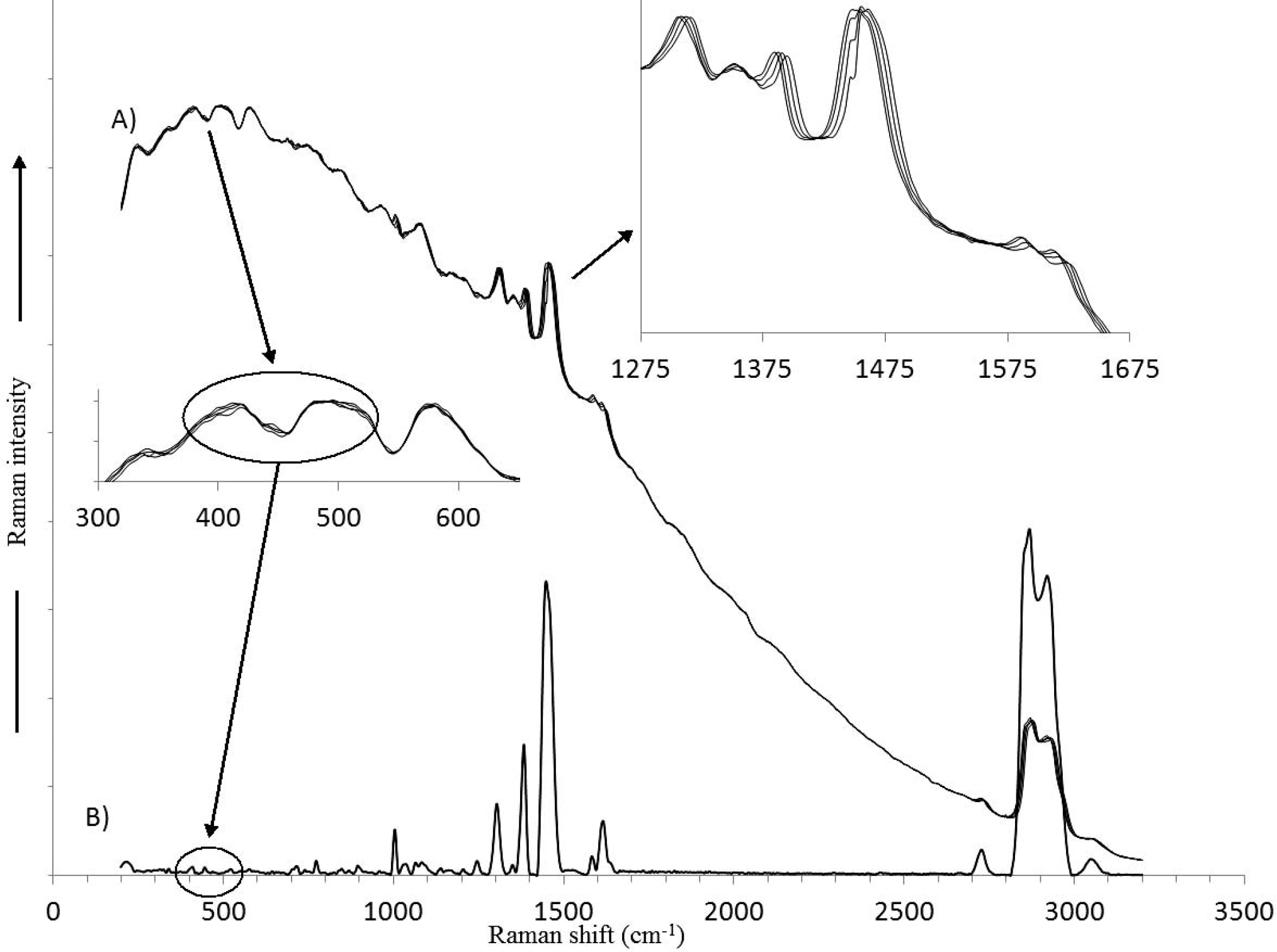
The Raman spectra of a diesel fuel are shown: (A) Four overlaid raw unprocessed Raman spectra and (B) the SSE Raman spectrum. Two expanded regions of the raw overlaid Raman spectra are shown in the insets. In one of the insets, a circle indicates the corresponding spectral region in the SSE Raman spectrum. The raw Raman spectra were acquired at four temperatures (22, 26, 30, and 34 °C) with an acquisition time of 15 s for each spectrum.

Perhaps an even more instructive sample is the inorganic salt ceric(IV) ammonium sulfate. The lanthanide metal cation exhibits very intense phosphorescence arising from the f-orbital electron transitions. In addition, the luminescence is structured with peaks that exhibit a similar bandwidth to Raman peaks. The luminescence extends well into the near-IR, giving an intense spectrum even when excited with 1064 nm radiation. Figure 8 shows the raw Raman spectra (Fig. 8A) as well as the SSE Raman spectrum (Fig. 8B) for this sample. An inset is included in Fig. 8 that expands the most intense spectral region of the raw Raman spectra (1175–1275 cm⁻¹). The lack of any obvious shifting of intensities in this region indicates that the sharp peaks are due predominantly to the luminescence. An inset is also included that expands the low wavenumber region (200–1100 cm⁻¹) of the raw Raman spectra. In order to see the Raman peaks in this region, the inset intensities are scaled by a factor of 50. For each shifting peak in the raw data, there is a corresponding peak in the SSE Raman spectrum. A third inset is included in Fig. 8 expanding the raw Raman spectral region 2350–2550 cm⁻¹. The intensities in this inset are scaled by a factor of 1000. A circle on this inset indicates where a shift would be expected for the small peak encircled on the SSE Raman spectrum (Fig. 8B). As can be seen, a shift is observed, but the intensity of the shifting peak is barely above the detection limit of the measurement due to the high noise level. Despite this, the SSE algorithm is able to extract the peak over the noise, which remains unshifted in the raw Raman spectra. This case clearly represents the defining limitation of the SSE method: Noise that results in an apparent sequential shift across a wavelength range of a bandwidth or more will result in an “artifact” peak. This type of noise limitation is distinctly different from traditional CCD Raman spectroscopy where the noise is typically Poisson distributed across the wavelength axis. The fact that the appearance of this peak is reproducible in subsequent measurements as well as its presence when no sample is placed in the glass vial suggests it can be attributed to the DBR laser. Although the laser is filtered with a filter that has an optical density (OD) of six, at this wavelength the OD of the filter drops to five. It can be seen from this example that the requirement for artifacts to appear involves the presence of noise (e.g., non-Raman signal) that is not random in terms of its frequency components along the wavelength axis and that this situation might occur as the detection limit of the measurement is approached. Considering this, it is difficult to know whether or not the intensities in the 1200–1700 cm⁻¹ range of the SSE Raman spectrum (Fig. 8B) are due to Raman scattering of the sample or noise since the fluorescence intensity being removed is ∼35 000 times more intense.

Fig. 8.

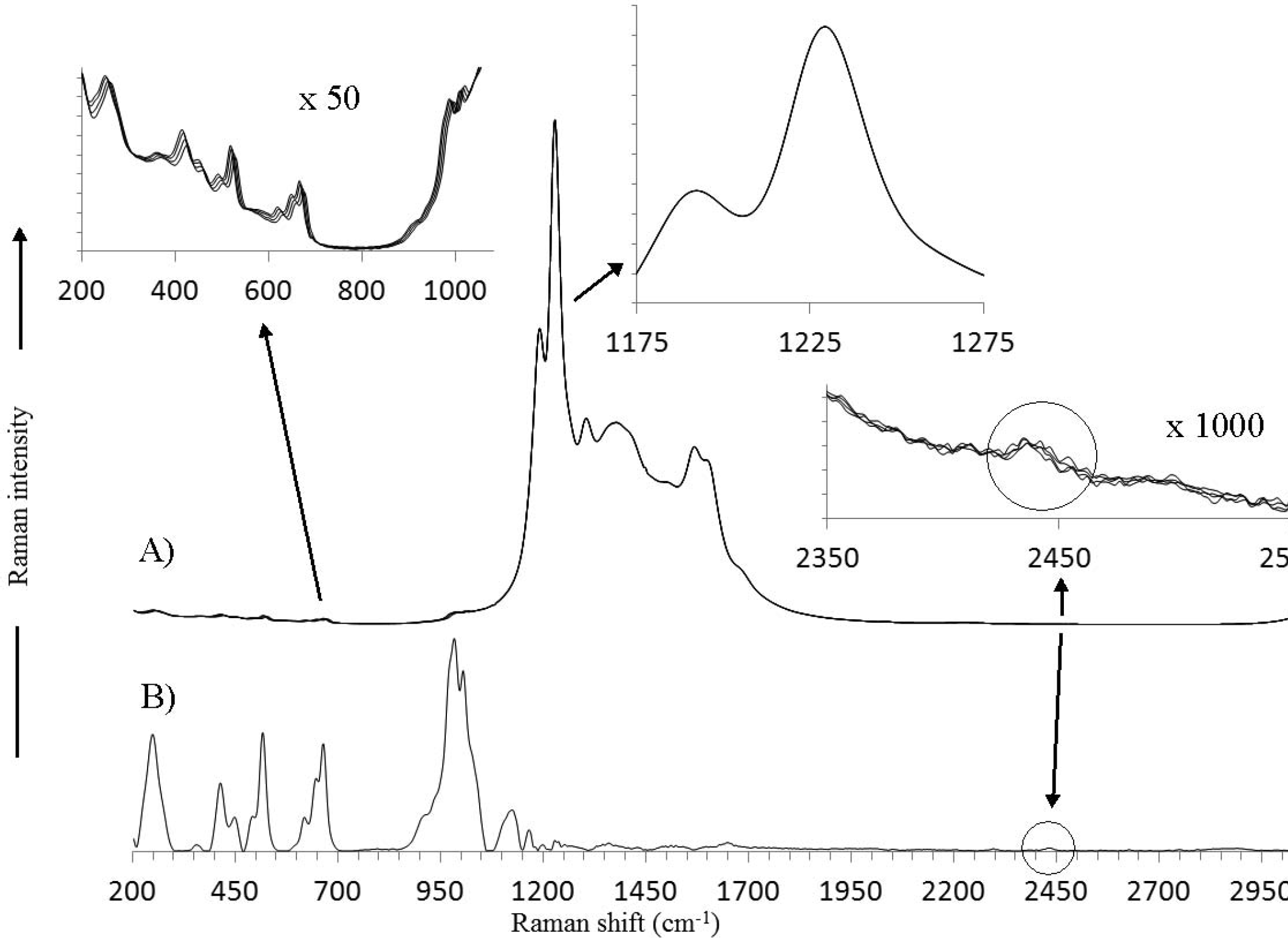
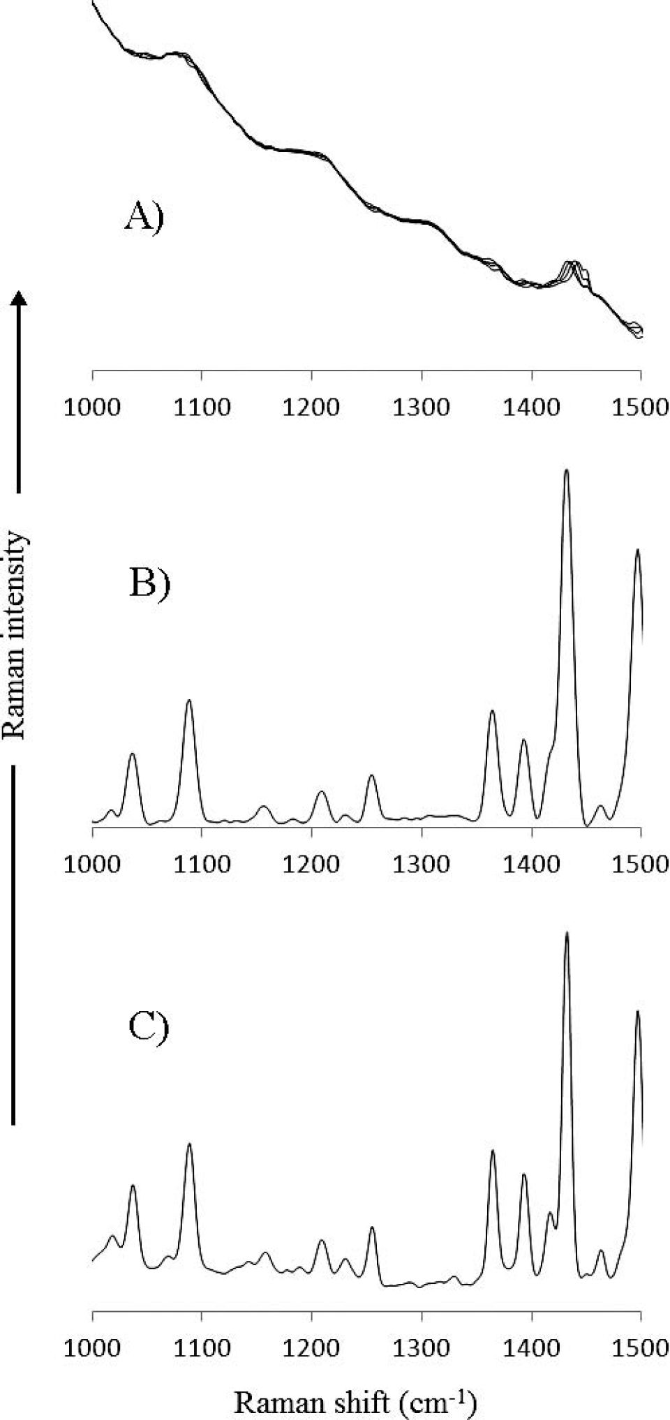
The Raman spectra of ceric(IV)ammonium sulfate (Ce(NH₄)₄(SO₄)₄. 2H₂O) are shown: (A) four overlaid raw unprocessed Raman spectra and (B) the SSE Raman spectrum. Three expanded regions of the raw overlaid Raman spectra are shown in the insets. In one of the insets, a circle is used to show the corresponding spectral region in the SSE Raman spectrum. The raw Raman spectra were acquired at four temperatures (22, 26, 30, and 34 °C) with an integration time of 0.5 s for each spectrum with a spectral average of 75 (total acquisition time of each spectrum is 18.75 s).

A similar situation testing the detection limit of a measurement is given in Fig. 4 for the highly fluorescent acenapthylene. Acenapthylene is a very difficult sample to measure not only due to its intense fluorescence, but also due to the fact that the fluorescence intensity and shape are highly dependent upon the crystallinity of the sample. In Fig. 9 the SSE Raman spectra of acenapthylene are shown as a function of the number of iterations used in the SSE calculation. The raw Raman spectra were acquired using a total acquisition time of 35.25 s per spectrum by averaging 75 spectra, each with an integration period of 0.47 s to avoid saturation of the 16 bit A/D converter. As shown, there are significant changes to the SSE Raman spectra at low iteration number, and even after 1000 iterations there are still distortions in several of the Raman bands. At 5000 iterations, the SSE Raman spectrum matches that of the FT-Raman spectrum (Fig. 4A) fairly well, and by 10 000 iterations no distortions or artifacts in the Raman spectrum can be observed, even though there is still some remaining underlying background (the increase of iteration number to 10 000 iterations results in a computation time of 3 s). Despite the remaining background, it is still significantly lower than that of the FT-Raman spectrum. Interestingly, only samples that have a poor S/N require more than 2000 iterations to reach a convergence point. The spectral range 1000–1500 cm⁻¹ contains both intense peaks as well as peaks with low S/N. This expanded spectral range is shown in Fig. 10A for the raw Raman spectra used to generate the SSE Raman spectra in Fig. 9. For comparison, the 5000-iteration SSE Raman is shown in Fig. 10B, and the FT-Raman spectrum is shown in Fig. 10C. Despite the low S/N in the raw Raman spectra, the SSE Raman shows a very high S/N. Indeed, a one-to-one comparison can be made between the peaks in the FT-Raman and the SSE Raman spectra. At very low intensities, it is difficult to know whether any slight differences between the spectra are due to noise in the FT-Raman spectrum or to artifacts in the SSE Raman spectrum.

Fig. 9.

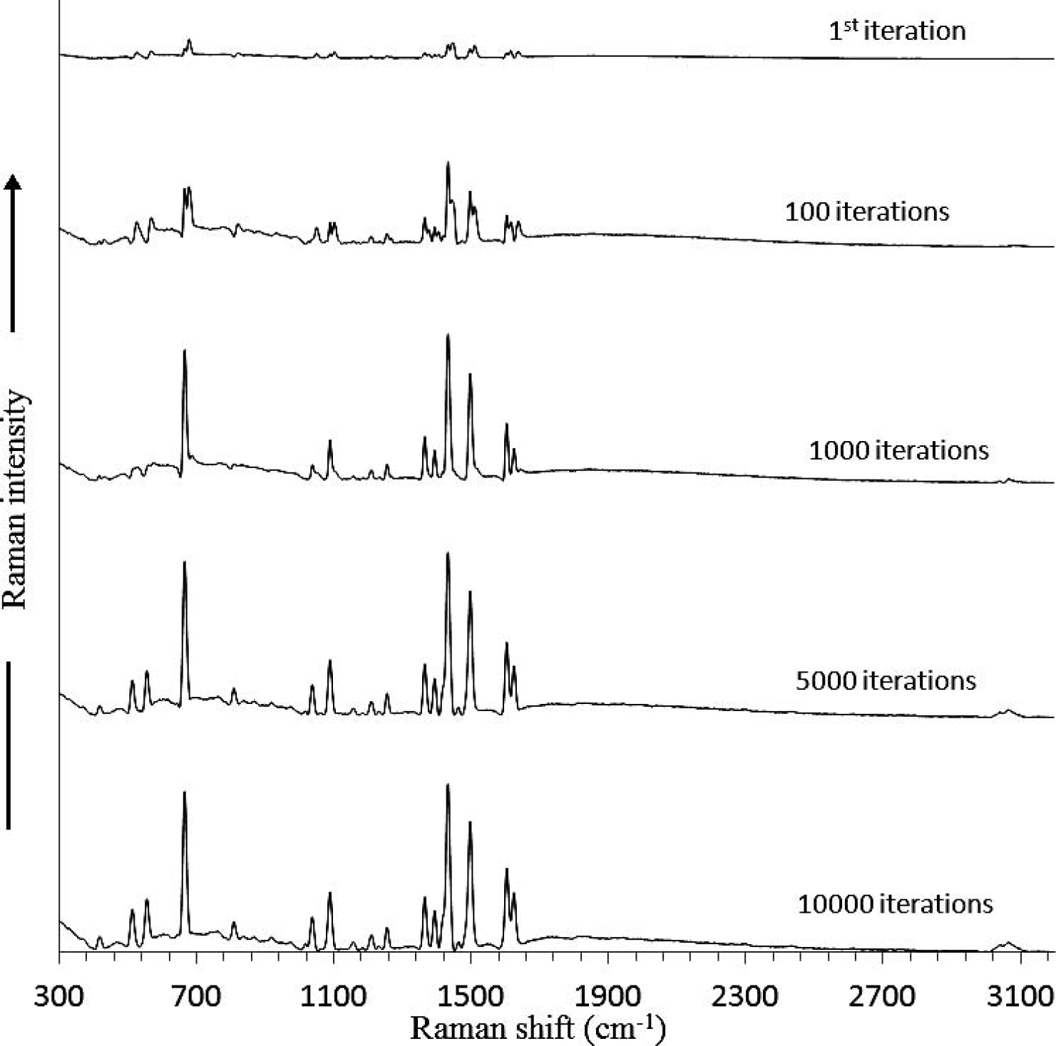
The SSE Raman spectra of acenapthylene using increasing iterations are shown. The Raman spectra used for SSE were acquired at four temperatures (22, 26, 30, and 34 °C) with a total acquisition time of 35.25 s for each spectrum (0.470 s integration time with 75 spectra averaged).

Fig. 10.

The spectral range 1000–1500 cm⁻¹ for the spectra of acenapthylene are shown for (A) the raw spectra used to generate the SSE Raman spectra shown in Fig. 9, (B) the 5000 iteration SSE Raman spectrum from Fig. 9, and (C) the FT-Raman spectrum shown in Fig. 4A.

In addition to the dependencies on S/N and iteration number, we have found that using the algorithms as presented in this paper, it is important to use temperatures that generate the same excitation shift for each sequential spectrum. Although one would expect Eq. 1 to give these temperatures, we have found that the polynomial calibration curves used to program the TEC are not always in compliance with the spectral data shifts and that it is often better to use a Raman standard such as acetaminophen to empirically determine small corrections to the temperatures in order to give the same shift with each sequential shift. If this is done, an increase in the number of excitations generally improves the results significantly for difficult samples,. These findings will be the subject of future work.

CONCLUSIONS

The major benefit of the SSE Raman method with the described instrumentation lies in its universal ability to extract Raman spectra from fluorescence interference using inexpensive and compact instrumentation in a time-efficient manner. The SSE method offers superior S/N performance when compared to shifted excitation methods that do not use iterative algorithms. With respect to the previous reports using iterative algorithms and shifted excitation, the SSE processing is three orders of magnitude faster due to its computational dependence on KN (compared to previous results that are dependent on KN²), resulting in sub-second processing times compared to processing times exceeding a minute. If derivative data are desired, it is possible to calculate the derivative using conventional algorithms, and any changes in the resulting bandwidth are dependent solely on the derivative algorithm used and not the experimental conditions. This is not the case with SERDS or PCA methods whose native derivative bandwidths and peak positions are dependent on the experimental conditions (excitations chosen). In addition, SSE Raman is the only method that allows all of the excitation conditions to be easily varied in a predefined manner (number of excitations, separation of excitations, and integration time of each excitation) in order to obtain optimal results. We have begun to investigate the impact of these parameters in order to gain a better understanding of optimal conditions for varied samples. As with other Raman extraction methods involving more than two excitations, even in the absence of a background, SSE Raman improves the S/N ratio by reducing random shot and thermal noise and by eliminating fixed pattern and random spike noise. In the current work, this allows an uncooled CCD detector to be used. The use of a cooled CCD would allow much longer integration times to be used for weak Raman scatters without having the thermal noise impact the dynamic range of the 16-bit A/D converter.

Importantly, the ability to tune the DBR laser to set wavelengths allows the excitation shift to be set to a constant value. This simplifies implementation of the iteration algorithms since the shift index of either the operator matrix (Eq. 8) or the weighting vector (Eqs. 9–11) can be set equal to the constant excitation shift (or an integral number multiplied times the excitation shift) and thus allow a single algorithm to be used even for different instruments. The only previous description of using shifted excitations with an iterative algorithm consisted of using eight single-mode excitation lasers with fixed wavelengths of 782.6, 784.1, 784.4, 786.8, 788.6, 790.7, 793.6, and 794.3 nm with three or more of the lasers being used to collect the Raman spectra. The use of multiple excitations of varying separations requires that the data be splined (or fitted) so that the spectral spacing is equal to the lowest common denominator of all excitation shifts that are used if equivalent results to SSE are to be obtained. Such a procedure results in an increase in N and is particularly ineffective when using Eq. 8 with calculation times that are proportional to KN².

References

Brody

R.H.

Carter

E.A.

Edwards

H.G.M.

Pollard

A.M.

. “FT-Raman Spectroscopy, Applications”. In: Lindon

J.C.

George

, editors. Online Encyclopedia of Spectroscopy and Spectrometry. Oxford, UK: Academic Press, 1999. Pp. 732.

Chase

. “FT-Raman Spectroscopy: A Catalyst for the Raman Explosion?” J. Chem. Ed. 2007. 84(1): 75–80.

Cooper

J.B.

Wise

K.L.

Jensen

B.J.

. “Modulated FT-Raman Fiber-Optic Spectroscopy: A Technique for Remotely Monitoring High-Temperature Reactions in Real-Time”. Anal. Chem. 1997. 69(11): 1973–1978.

Lewis

M.L.

Lewis

I.R.

Griffiths

P.R.

. “Raman Spectrometry of Explosives with a No-Moving-Parts Fiber Coupled Spectrometer: A Comparison of Excitation Wavelength”. Vibr. Spectr. 2005. 38(1/2): 17–28.

Hasegawa

Nishijo

Umemura

. “Separation of Raman Spectra from Fluorescence Emission Background by Principal Component Analysis”. Chem. Phys. Lett. 2000. 317(6): 642–646.

Zhao

Harvey

McLean

D.I.

Zeng

. “Automated Autofluorescence Background Subtraction Algorithm for Biomedical Raman Spectroscopy”. Appl. Spectr. 2007. 61(11): 1225–1232.

Zhao

Lui

McLean

D.I.

Zeng

. “Integrated Real-Time Raman System for Clinical In Vivo Skin Analysis”. Skin Res. Tech. 2008. 14(4): 484–492.

Lieber

C.A.

Mahadevan-Jansen

. “Automated Method for Subtraction of Fluorescence from Biological Raman Spectra”. Appl. Spectrosc. 2003. 57(11): 1363–1367.

Mosier-Boss

P.A.

Lieberman

S.H.

Newberry

. “Fluorescence Rejection in Raman Spectroscopy by Shifted-Spectra, Edge Detection, and FFT Filtering Techniques”. Appl. Spectr. 1995. 49(5): 630–638.

10.

Schulze

H.G.

Foist

R.B.

Okuda

Ivanov

Turner

R.F.

. “A Model-Free, Fully Automated Baseline-Removal Method for Raman Spectra”. Appl. Spectr. 2011. 65(1): 75–84.

11.

Zhang

Ben-Amotz

. “Enhanced Chemical Classification of Raman Images in the Presence of Strong Fluorescence Interference”. Appl. Spectr. 2000. 54(9): 1379–1383.

12.

Zhang

Z.-M.

Chen

Liang

Y.-Z.

Liu

Z.-X.

Zhang

Q.-M.

Ding

L.-X.

Zhou

. “An Intelligent Background-Correction Algorithm for Highly Fluorescent Samples in Raman Spectroscopy”. J. Raman Spectr. 2010. 41(6): 659–669.

13.

Cormack

I.G.

Mazilu

Dholakia

Herrington

C.S.

. “Fluorescence Suppression within Raman Spectroscopy Using Annular Beam Excitation”. Appl. Phys. Lett. 2007. 91(2): 023903. doi: 10.1063/1.2756311.

14.

Le Ru

E.C.

Schroeter

L.C.

Etchegoin

P.G.

. “Direct Measurement of Resonance Raman Spectra and Cross Sections by a Polarization Difference Technique”. Anal. Chem. 2012. 84(11): 5074–5079.

15.

Schulmerich

M.V.

Reddy

Kodali

A.K.

Elgass

L.J.

Tangella

Bhargava

. “Dark Field Raman Microscopy”. Anal. Chem. 2010. 82(14): 6273–6280.

16.

Lakshmanna

Mallick

Umapathy

. “Ultrafast Raman Loss Spectroscopy: A New Approach to Vibrational Structure Determination”. Curr. Sci. 2009. 97(2): 210–216.

17.

Mandal

Mizuno

Tahara

. “Temporal Fluorescence Rejection in Raman Spectroscopy Using Femtosecond Up-Conversion with Single- and Multi-Channel Detection”. J. Mol. Struc. 2005. 735–736: 189–195.

18.

Martyshkin

D.V.

Ahuja

R.C.

Kudriavtsev

Mirov

S.B.

. “Effective Suppression of Fluorescence Light in Raman Measurements Using Ultrafast Time Gated Charge Coupled Device Camera”. Rev. Sci. Instr. 2004. 75(3): 630–636.

19.

McCamant

D.W.

Kukura

Yoon

Mathies

R.A.

. “Femtosecond Broadband Stimulated Raman Spectroscopy: Apparatus and Methods”. Rev. Sci. Instr. 2004. 75(11): 4971–4980.

20.

Misra

A.K.

Sharma

S.K.

Chio

C.H.

Lucey

P.G.

Lienert

. “Pulsed Remote Raman System for Daytime Measurements of Mineral Spectra”. Spectrochim. Acta A. 2005. 61(10): 2281–2287.

21.

Vikman

Iitti

Matousek

Towrie

Parker

A.W.

Vuorinen

. “Kerr Gated Resonance Raman Spectroscopy in Light Fastness Studies of Ink Jet Prints”. Vibr. Spectr. 2005. 37(1): 123–131.

22.

Canetta

Mazilu

De Luca

A.C.

Carruthers

A.E.

Dholakia

Neilson

Sargeant

Briscoe

Herrington

C.S.

Riches

A.C.

. “Modulated Raman Spectroscopy for Enhanced Identification of Bladder Tumor Cells in Urine Samples”. J. Biomed. Optics. 2011. 16(3): 037002. doi: 10.1117/1.3556722.

23.

Chen

C.G.

Sedlacek

A.J.

III . “Revisiting Raman Lidar: Application of New Techniques to Improve System Performance”. Proc. SPIE. 2833, Application of Lidar to Current Atmospheric Topics (November 12, 1996): 182–192. doi:10.1117/12.258154.

24.

De Luca

A.C.

Mazilu

Riches

. “Online Fluorescence Suppression in Modulated Raman Spectroscopy”. Anal. Chem. 2010. 82(2): 738–745.

25.

Funfschilling

Williams

D.F.

. “CW Laser Wavelength Modulation in Raman and Site Selection Fluorescence Spectroscopy”. Appl. Spectr. 1976. 30(4): 443–446.

26.

Kamogawa

Fujii

Kitagawa

. “Improved Fluorescence Rejection in Measurements of Raman Spectra of Fluorescent Compounds”. Appl. Spectr. 1988. 42(2): 248–254.

27.

Maiwald

Erbert

Klehr

Kronfeldt

H.D.

Schmidt

Sumpf

Traenkle

. “Rapid Shifted Excitation Raman Difference Spectroscopy with a Distributed Feedback Diode Laser Emitting at 785 nm”. Appl. Phys. B. 2006. 85: 509–512.

28.

Maiwald

Schmidt

Sumpf

. “Microsystem 671 nm Light Source for Shifted Excitation Raman Difference Spectroscopy”. Appl. Optics. 2009. 48(15): 2789–2792.

29.

Matousek

Towrie

Parker

A.W.

. “Simple Reconstruction Algorithm for Shifted Excitation Raman Difference Spectroscopy”. Appl. Spectr. 2005. 59(6): 848–851.

30.

Mazilu

L.A.C.

Riches

Herrington

Dholakia

Farkas

D.L.

Nicolau

D.V.

Leif

R.C.

. “Modulated Raman Spectroscopy Technique for Real-Time Fluorescence Rejection”. Proc. SPIE. 7568, Imaging, Manipulation, and Analysis of Biomolecules, Cells, and Tissues VIII (February 24, 2010): 75680M. doi:10.1117/12.841675.

31.

Mazilu

De Luca

A.C.

Riches

Herrington

C.S.

Dholakia

. “Optimal Algorithm for Fluorescence Suppression of Modulated Raman Spectroscopy”. Opt. Express. 2010. 18(11): 11382–11395.

32.

McCain

S.T.

Willett

R.M.

Brady

D.J.

. “Multi-Excitation Raman Spectroscopy Technique for Fluorescence Rejection”. Opt. Express. 2008. 16(15): 10975–10991.

33.

Michaelian

K.H.

Yuan

Hall

R.H.

Bulmer

J.T.

. “Fluorescence Rejection in Raman Spectra of Syncrude Sweet Blend Distillation Fractions”. Spectrochim. Acta A. 2005. 62(1–3): 582–591.

34.

Oshima

Komachi

Furihata

Tashiro

Sato

. “Fluorescence-Suppressed Raman Technique for Quantitative Analysis of Protein Solution Using a Micro-Raman Probe, the Shifted Excitation Method, and Partial Least Squares Regression Analysis”. Appl. Spectr. 2006. 60(9): 964–970.

35.

Osticioli

Zoppi

Castellucci

E.M.

. “Shift-Excitation Raman Difference Spectroscopy Difference Deconvolution Method for the Luminescence Background Rejection from Raman Spectra of Solid Samples”. Appl. Spectr. 2007. 61(8): 839–844.

36.

Shreve

A.P.

Cherepy

N.J.

Mathies

R.A.

. “Effective Rejection of Fluorescence Interference in Raman Spectroscopy Using a Shifted Excitation Difference Technique”. Appl. Spectr. 1992. 46(4): 707–711.

37.

Stellman

C.M.

Bucholtz

. “Suppression of Fluorescence Interference via Wavelength Shift-Keyed Raman Spectroscopy Using an Argon Ion Laser and Acousto-Optic Tunable Filter”. Spectrochim. Acta A. 1998. 54(8): 1041–1047.

38.

Willett

. “Multiscale Reconstruction for Photon-Limited Shifted Excitation Raman Spectroscopy”. In: IEEE International Conference on Acoustics, Speech and Signal Processing. ICASSP, 2007. Pp. III.

39.

Xie

Y.-Q.

, “Confocal Micro-Raman Spectroscopy of Single Biological Cells Using Optical Trapping and Shifted Excitation Difference Techniques”. J. Appl. Phys. 2003. 93(5): 2982–2986.

40.

Zhao

Carrabba

M.M.

Allen

F.S.

. “Automated Fluorescence Rejection Using Shifted Excitation Raman Difference Spectroscopy”. Appl. Spectr. 2002. 56(7): 834–845.

41.

Zou

Cai

. “Fluorescence Rejection by Shifted Excitation Raman Difference Spectroscopy”. Proc. SPIE. 2010. 7855: 78551M.

42.

Osticioli

Zoppi

Castellucci

E.M.

. “Fluorescence and Raman Spectra on Painting Materials: Reconstruction of Spectra with Mathematical Methods”. J. Raman Spectr. 2006. 37(10): 974–980.

43.

Martins

M.A. d. S.

Ribeiro

D.G.

Pereira dos Santos

E.A.

Martin

A.A.

Fontes

Martinho

H. d. S.

. “Shifted-Excitation Raman Difference Spectroscopy for In Vitro and In Vivo Biological Samples Analysis”. Biomed. Opt. Express. 2010. 1(2): 617–626.