Modeling Metal Binding by Dissolved Humic Substance: A Revisit to the Fluorometric Titration Approach

Abstract

It is desirable to directly investigate metal cation binding by dissolved humic substance (HS) in environmental samples without isolation and purification of the HS. This is commonly achieved by the fluorometric titration approach, in which the variations of the HS components' fluorescence when titrated with metal cations, such as cupric ions (Cu²⁺), were commonly resolved by a well-established chemometric tool called parallel factor analysis and fit to a classical nonlin ear equation to obtain cation binding parameters. The nonlinear expression was derived based on the two assumptions that a given HS component (e.g., L) binds Cu²⁺ with a 1:1 stoichiometry, forming only the complex LCu, and that other ligands competing with L for Cu²⁺ are not explicitly considered. Given the deviations (e.g., the presence of multiple HS components competing for Cu²⁺ and a likely 2:1 binding stoichiometry in addition to the 1:1 binding) from the assumptions, the fitting-derived binding parameters reported in past studies are questionable; those studies commonly reported high goodness-of-fit (R²) as a support of the validity of the assumptions. This study deconstructed the current equation and examined it with two organic ligand components in a simulated study to see what conditions could also yield a good fit. It turned out that high a R² value ranging between 0.9971 and 1.0 was observed despite the deviations from the above-mentioned assumptions. In addition, this study re-evaluated some published experimental data from these past studies and found that the fitting-derived parameters could not be accounted for based on the above-mentioned assumptions. The findings in this study therefore indicate that the current fluorometric titration approach is problematic when investigating HS component interactions with metal ions in situ. The combination of ion-selective electrode and fluorometric titration may be an alternative to the current fluorometric titration approach alone.

Keywords

Humic substance Metal binding Fluorometric titration Parallel factor analysis PARAFAC

INTRODUCTION

Dissolved humic substances (HS) are ubiquitous in ecosystems, comprises a large fraction (50∼80% in terms of organic carbon) of the total dissolved organic matter (DOM) pool.¹ and plays essential roles in the environment. Metal binding by dissolved HS affects the speciation of toxic metals² and, in turn, their bioavailability.^3–5 Indeed, metal binding by HS is a key issue considered in biotic ligand models used to predict the site-specific toxicity of metals or to derive site-specific ambient water quality criteria.^6–9

The HS generated in different environment or sites may differ considerably in chemical properties and thus metal-binding characteristics, and it may show different abilities to protect organisms against heavy metal toxicity.¹⁰ It is desirable to use a technical approach that enables selective monitoring of metal binding by HS components (e.g., humic acid and fulvic acid) in environmental samples and does not require isolation and purification of HS components from samples, thereby not giving rise to alterations to metal-binding characteristics of the HS components. To this end, fluorometric titration of HS by metal ion(s) (M) holds promise,^11,12 because HS fluorescence variations induced by metal binding to HS can be monitored in situ and exploited to derive the binding parameters.

By simply assuming that M was bound only by a single organic molecule (L) representative of the investigated HS sample and that the binding stoichiometry between L and M was 1:1, Ryan and Weber^11,13 introduced a quadratic equation (hereafter RW) for data fitting. This approach could give operationally defined binding parameters (i.e., K, the conditional formation constant of the complex LM; C_L, the total concentration of L; and I_ML, the residual fluorescence of LM relative to free L) given experimentally controlled variables, observed variables, or both (i.e., C_M, the total added concentration of M; and F, the observed total fluorescence of L+LM at each titration step). This approach was adopted in many later DOM studies.^14,15

However, some studies^16–18 realized that the fitting-derived binding parameters depended on the excitation and emission wavelength pair used for measuring F. Such wavelength dependence was attributed to the competition among multiple HS components for binding M; these components could not be well distinguished by a single wavelength pair because they showed overlapping spectra.

To solve the spectral overlapping problem, a well-established multivariate statistical technique called parallel factor analysis (PARAFAC) for analysis of fluorescence excitation–emission matrix (EEM) was invoked.^19–28 In those studies, EEMs of the metal-titrated samples were decomposed by PARAFAC to show how fluorescence of a given HS component changed with the titration; each component was usually fit to the classical RW equation. The joint application of the RW equation and PARAFAC is referred to as the RW-PARAFAC approach hereafter.

Given the likelihood that metal was bound by multiple components, there would be a deviation from the classical assumptions for the RW equation, let alone the likely binding stoichiometry other than 1:1. Therefore, the binding parameters of the HS components reported by studies using the RW-PARAFAC approach were problematic. Surprisingly, the fitting usually showed high (e.g., >0.99) values of goodness-of-fit (R²)^20,23 that were considered (implicitly or explicitly) supportive of the assumptions for the RW equation.

Given the uncertainty as to whether one could use R² values alone to justify the assumptions, the present study had two objectives. The first objective was to simulate metal titration and data fitting in a hypothetical two-component HS sample to explore whether a good fit could still be obtained under scenarios very different from the classical assumptions. The second objective was to re-evaluate the reliability of some published binding parameters derived from the RW-PARAFAC approach applied to real experimental data.

MATERIALS AND METHODS

Simulation. All the computation required for the hypothetical experiment was achieved using in-house routines in the software package of Matlab 6.5 (The MathWorks, Natick, MA). Given that Cu²⁺ is the most widely investigated metal ion in this context, the present study used Cu²⁺ as a model metal for the simulation study. As analyzed in detail (see Supplemental Material), the C_L and K values obtained by fitting the fluorescence response curve to the RW equation would by no means be invariant. Instead, they were expected to vary, depending not only on the sub-range of the total added Cu²⁺ concentration (C_Cu) used for the data fitting but also on chemical reactions competing with the formation of LCu. To avoid confusion, C_L* and K* are used herein to refer to the fitting-derived two operational parameters for C_L and K.

The whole simulation did not involve the PARAFAC modeling of EEMs. Instead, it was only focused on synthesizing and fitting a hypothetical fluorescence–response curve of the target component L plus LM in the Cu²⁺ titration in the presence of competing organic ligand A. The key issue of the whole problem was post-PARAFAC pertinent to analysis and interpretation of the response curve based on the classical RW equation.

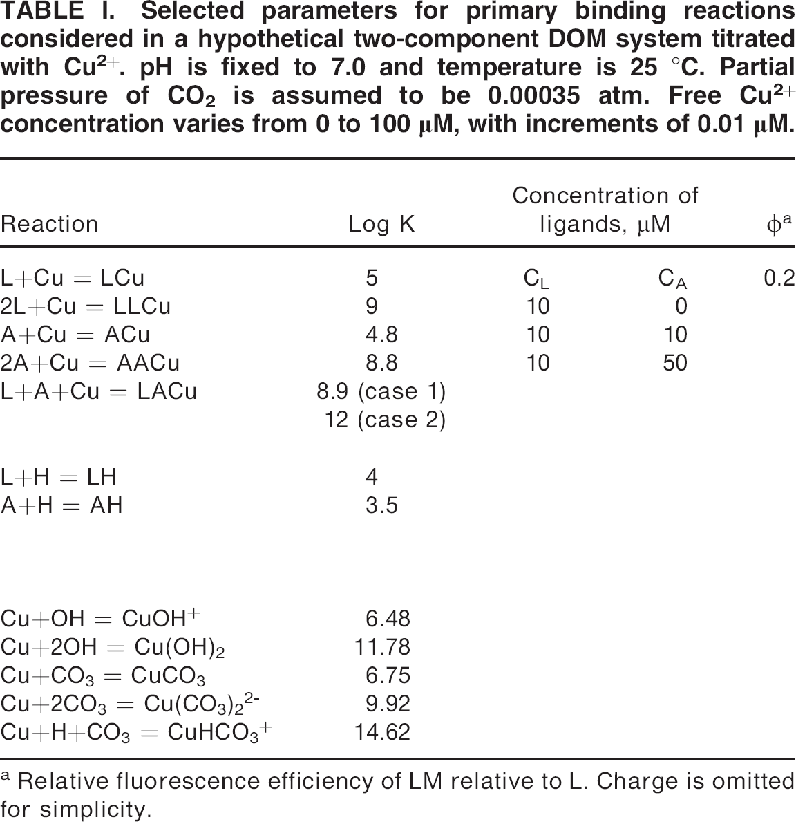
Hypothetically, Cu²⁺ was added into an HS solution consisting of two components, with one component being the target organic molecule L of interest and the other component being the competing organic molecule A. The complexation of Cu²⁺ by typical inorganic ligands was taken into account (Table I). The cumulative formation constants for complexation reactions were adopted from the chemical equilibria database, the Windermere Humic Aqueous Model, version 7 (WHAM7). The concentration of carbonate (i.e., [CO₃^2–]) was estimated (see Supplemental Material).

TABLE I.

Selected parameters for primary binding reactions considered in a hypothetical two-component DOM system titrated with Cu²⁺. pH is fixed to 7.0 and temperature is 25 °C. Partial pressure of CO₂ is assumed to be 0.00035 atm. Free Cu²⁺ concentration varies from 0 to 100 μM, with increments of 0.01 μM.

Reaction	Log K	Concentration of ligands, μM		φ^a
L+Cu = LCu	5	C_L	C_A	0.2
2L+Cu = LLCu	9	10	0
A+Cu = ACu	4.8	10	10
2A+Cu = AACu	8.8	10	50
L+A+Cu = LACu	8.9 (case 1)
	12 (case 2)
L+H = LH	4
A+H = AH	3.5
Cu+OH = CuOH⁺	6.48
Cu+2OH = Cu(OH)₂	11.78
Cu+CO₃ = CuCO₃	6.75
Cu+2CO₃ = Cu(CO₃)₂^2-	9.92
Cu+H+CO₃ = CuHCO₃⁺	14.62

Relative fluorescence efficiency of LM relative to L. Charge is omitted for simplicity.

Seven reactions involving organic ligands (Table I) were considered: three reactions related to ligand L's binding to Cu²⁺ and hydrogen ion H (Eqs. I –III), three reactions related to ligand A's binding to Cu²⁺ and hydrogen ion H (Eqs. IV –VI), and one reaction related to the mixed binding of Cu²⁺ (Eq. VII). The protonation of L was assumed to be monoprotic in this study, because HS acid–base properties are commonly well interpreted by assuming HS to be a mixture of monoprotic acids.^29,30

For simplicity, we used K_i hereinafter to refer to the formation constant of the following i^th (i = I, II,…VII) reaction, for which the charge was omitted to avoid confusion. Cu²⁺ binding by inorganic ligands was also considered in the simulation (Table I) but is not addressed here for simplicity.

L + Cu = LCu

(I)

2 L + Cu = L_{2} Cu

(II)

L + H = LH

(III)

A + Cu = ACu

(IV)

2 A + Cu = A_{2} Cu

(V)

A + H = AH

(VI)

L + A + Cu = LACu

(VII)

In the simulation, we used the strategy that the free Cu²⁺ concentration [Cu] was preset while looking for the total added Cu²⁺ (C_Cu), based on the relevant chemical equilibria (Table I), given the knowledge of the total concentrations of the organic ligands (e.g., C_L and C_A), pH, and the partial pressure of CO₂ at a constant temperature of 25 °C. The hypothetical fluorescence–response curve of the hypothetical PARAFAC component L was constructed based on the computed C_Cu, with a premise that only the free L and complex LM contribute to the observed fluorescence of the target component L. Cu organic complexes of 2:1 stoichiometry (i.e., LLCu and LACu) were assumed to either show negligible fluorescence or fluoresce at spectral regions that were very different from those of L and LM. Our strategy was different from a presumably more traditional strategy that otherwise looks for the [Cu] at each titration step given preset values of C_Cu. Our strategy was adopted in the present study mainly because it facilitated the numeric computation in the presence of a variety of chemical equilibria. The procedure for finding the C_Cu is described as follows.

According to mass balance of L and A, we have

\begin{array}{l} C_{L} = K_{I} \times [L] [Cu] + 2 \times K_{II} \times {[L]}^{2} [Cu] \\ + K_{III} \times [L] [H] + K_{VII} \times [L] [A] [Cu] + [L] \end{array}

(1)

\begin{array}{l} C_{A} = K_{IV} \times [A] [Cu] + 2 \times K_{V} \times {[A]}^{2} [Cu] \\ + K_{VI} \times [A] [H] + K_{VII} \times [L] [A] [Cu] + [A] \end{array}

(2)

Rearranging Eq. 1, [A] can be expressed in terms of other variables as follows:

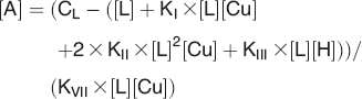
\begin{array}{l} [A] = (C_{L} - ([L] + K_{I} \times [L] [Cu] \\ + 2 \times K_{II} \times {[L]}^{2} [Cu] + K_{III} \times [L] [H])) / \\ (K_{VII} \times [L] [Cu]) \end{array}

(3)

In contrast, Eq. 2 is a quadratic equation of [A], and [A] can be readily obtained by solving the Eq. 2 in Matlab. Provided that an “optimum” [L] is correctly found, [A] obtained by Eq. 3 or Eq. 2 will be the same within computational errors. Following this logic, the Matlab built-in command fminbnd was used that varied [L] during the computation until the ratio between the above-mentioned two values of calculated [A] was close to unity (within an error of 10⁻⁶). After obtaining the “optimum” [L], the concentrations of the species (e.g., LCu) in the titration system can be readily obtained, and as such the C_Cu can be obtained by summing up the concentrations of all of the Cu²⁺ species.

The LCu fluorescence efficiency was set to 20% (i.e., φ = 0.2) of that of L in the simulation, based on the experimentally observed φ = 0.2 (at pH 7) for Suwannee River fulvic acid.¹¹ Therefore, starting from the initial fluorescence I₀ at C_Cu = 0 μM, the total fluorescence (I) of L plus LCu would decrease with titration of Cu²⁺.

As listed in Table I, the log K_VII for the mixed ligand binding (L+A+Cu = LACu) was set to two different values for comparison, i.e., log K_VII = 8.9 (case 1) or log K_VII = 12 (case 2). The value of K_VII in case 1 was set to be comparable to K_II and K_V, whereas in case 2 the value was set to be much higher than either of K_II and K_V, thereby indicating a higher stability of the ternary mixed ligand organic Cu²⁺ complex than the pure ligand complex. In addition, different values of C_A (Table I) were considered to investigate the effect of the solution composition on the fitting for the target component L.

Choice of a proper C_Cu range may be practically relevant when fitting real experimental data to the RW equation (equation shown in Supplemental Material), because the 2:1 binding is expected to become less important relative to the 1:1 binding when the ratio of C_Cu to binding molecules increases. The ratio of C_Cu to DOM was proven to play an important role in influencing the speciation of Cu²⁺ in natural waters and thereby the toxicity to aquatic organisms.³¹ Therefore, the influence of chosen C_Cu ranges on the fit was also evaluated in this study. Three C_Cu ranges were compared: 0∼40, 0∼80, and 0∼120 μM.

Experimental Data Re-evaluation. For a given HS component L, the PARAFAC-recovered relative fluorescence intensities of the component before metal titration were expected to be proportional to the fitting-derived C_L* based on the RW equation, and thus the fluorescence ratio between two components should covary with the C_L* ratio across the samples, if the assumptions of the RW equation were truly valid (see Supplementary Material for details). Based on this viewpoint, literature studies reporting both C_L and fluorescence intensity were screened for re-evaluation.

RESULTS

Simulation. The fluorescence–response curves (I/I₀ vs. C_Cu) of L and LCu for case 1 and case 2 are plotted in Figs. 1a and 1b, respectively. Fitting the synthetic fluorescence data (Fig. 1) to the RW equation was achieved with success, showing high values of adjusted R² that ranged from 0.9991 to 1.0 for most of the fits except for the fit (R² = 0.9971) at C_A = 10 μM and the C_Cu range of 0∼120 μM in case 2. Fitting-derived log K* and C_L* for each C_Cu range in each case are listed for better illustration in Tables II and III, respectively, whereas φ is plotted in Fig. 2.

Fig. 1.

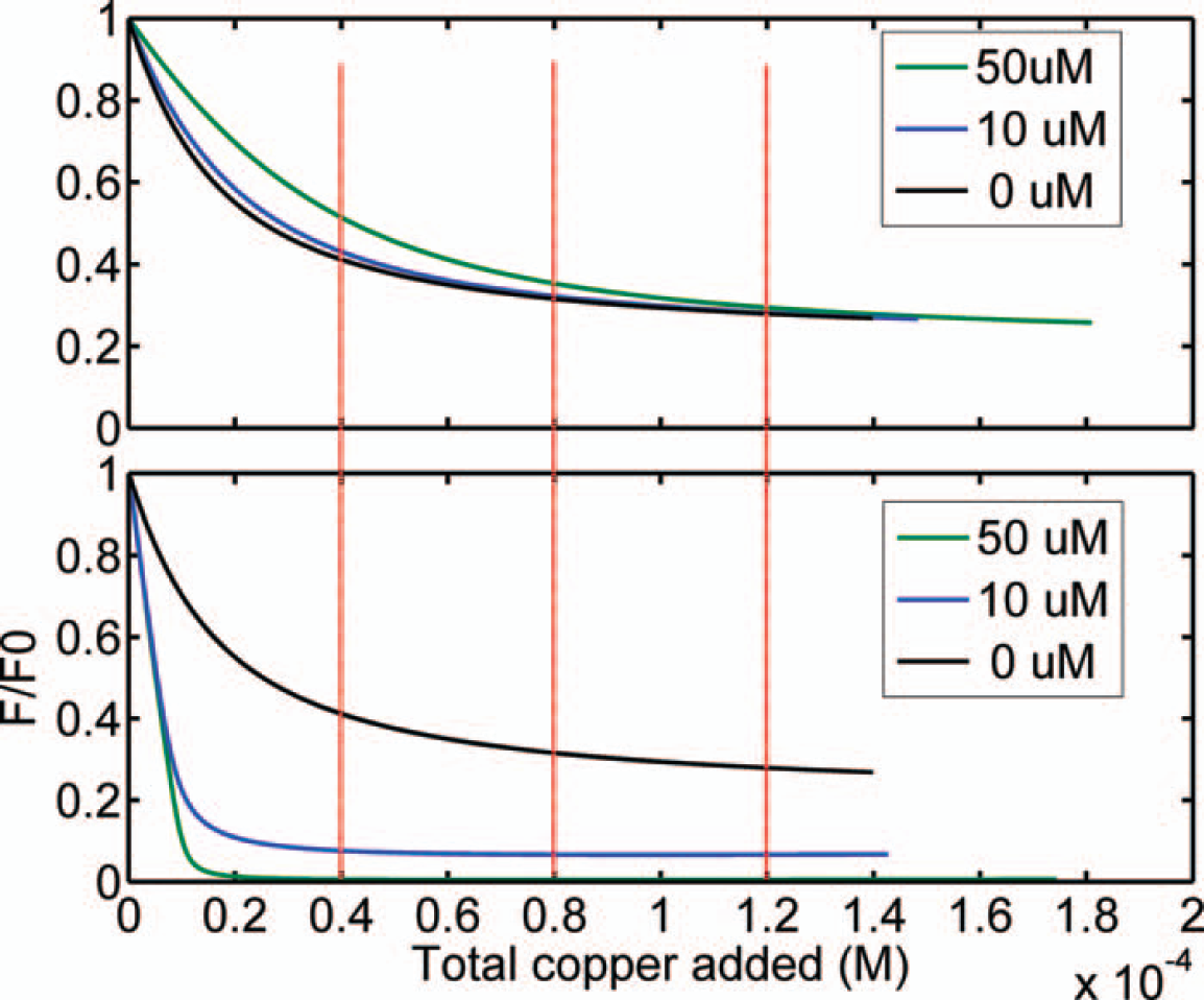
F/F0 (L and LCu) vs. total added Cu²⁺ concentration (L's total concentration = 10 μM) in a hypothetical two-component (L and A) DOM sample titrated by Cu²⁺. The competing molecule A has a total concentration of 0, 10, and 50 μM, respectively. Log of the formation constant of LAM is assumed to be 8.9 (case 1, top) or 12 (case 2, bottom). Dotted lines are shown to only delineate the differing Cu²⁺ concentration ranges to use in later data fitting.

Fig. 2.

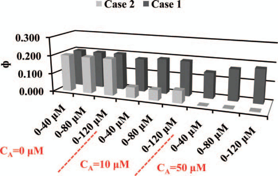
Fitting-derived φ values for the complex LCu. Three concentration ranges (0∼40, 0∼80, and 0∼120 μM) of added Cu²⁺ were used for modeling in the presence of a competing ligand A at total concentrations of 0, 10, and 50 μM, respectively. The formation constant of the complex LACu is set to 10^8.9 (case 1) or 10¹² (case 2).

TABLE II.

Fitting-derived log K* of target ligand L in the presence of a competing ligand A at varying concentrations (0, 10 and 50 μM). The true formation constant of the complex LACu was set to 10^8.9 (case 1) or 10¹² (case 2).

	C_A at 0 μM			C_A at 10 μM			C_A at 50 μM
Total Cu²⁺ range (μM)^a	0–40	0–80	0–120	0–40	0–80	0–120	0–40	0–80	0–120
Log K* in case 1	4.90	4.90	4.90	4.84	4.86	4.85	4.73	4.79	4.82
Log K* in case 2	4.90	4.90	4.90	6.18	6.17	6.28	6.93	6.95	6.97

Three different concentration ranges of total added Cu²⁺ were used for the fitting for comparison.

TABLE III.

Fitting-derived C_L* of target ligand L in the presence of a competing ligand A at varying concentrations (0, 10, and 50 μM). The true formation constant of the complex LACu was set to 10^8.9 (case 1) or 10¹² (case 2).

	C_A at 0 μM			C_A at 10 μM			C_A at 50 μM
Total Cu²⁺ range (μM)^a	0–40	0–80	0–120	0–40	0–80	0–120	0–40	0–80	0–120
CL* (μM) in case 1	6.88	6.72	6.74	10.04	10.52	9.76	28.10	29.22	30.28
CL* (μM) in case 1	6.88	6.72	6.74	8.50	8.45	9.10	10.01	10.04	10.05

Three different concentration ranges of total added Cu²⁺ were used for comparison.

As shown in Table II, log K* showed small variation (4.84 ± 0.06) and weak dependence on both of the C_Cu range and the C_A concentration in case 1. On the contrary, in case 2, log K* showed large variations with respect to C_A but still small variations with respect to C_Cu. It was evident that the log K* values were relatively invariant with respect to C_Cu in both cases.

The fitting-derived C_L* values (Table III) behaved differently from log K* in terms of dependence on C_A or C_Cu. Any two C_A values differed significantly (p < 0.01; paired t-test) in terms of affecting the fitting-derived C_L* values (increasing with C_A) in each case. In contrast, any two ranges of C_Cu did not differ significantly (p > 0.35, paired t-test) in terms of affecting the fitting-derived C_L* values, and no consistent trend of C_L* vs. C_Cu was observed. The fitting-derived C_L* was close to 10 μM only at C_A = 10 μM in case 1 (10.1 ± 0.4 μM) or at C_A = 50 μM in case 2 (10.0 ± 0.02 μM); otherwise, it was either much higher (29.2 ± 1.1 μM at C_A = 50 μM in case 1) or lower than 10 μM.

The value of φ (Fig. 2), in contrast, did not show any similar trend as the fitting-derived ogK* or C_L*. It fluctuated from values close to 0.20 (i.e., 0.199 ± 0.0007 at C_A = 0 μM in case 1 and case 2, 0.186 ± 0.005 at C_A = 10 μM in case 1) to near zero (0.001 ± 0.002 at C_A = 50 μM in case 2), but it did not exceed the true value of 0.20. It was noteworthy that in case 2, the φ values in the case of C_A = 10 μM and C_A = 50 μM (Fig. 2) were much lower than the true value of 0.20, and these low values seemed to compensate for the aforementioned high values of log K* to give equally good fitting.

Literature Experimental Data Re-evaluation. Two relevant studies were selected for data re-evaluation. One study was by Wu et al.²⁴ who investigated metal binding by fresh and aged municipal solid waste leachate DOM that was fractionated by ultrafiltration according to the apparent molecular size. Six PARAFAC-modeled fluorescent components were distributed across the fractions (fresh or aged) and showed large fluorescence abundance variability; two HS-like components C1 and C2 as termed in that study²⁴ were selected for further analysis in this study. The fluorescence ratios of C1 to C2 and the C_L* ratios of C1 to C2 (as determined by Cu²⁺ titration using the RW equation) in some size fractions are listed for comparison (Table IV).

TABLE IV.

Sample-dependent ratios between two HS-like components in terms of PARAFAC-identified fluorescence abundance or fitting-derived binding parameter C^L*.^a

	HS components in municipal solid waste leachate, kDA^b						HS components in fulvic acids^c

	Fresh			Aged

	<0.5	3–10	>10	<0.5	3–10	>10	SRFA	PLFA
Ratio between the two PARAFAC components' abundances	1.12	0.56	0.47	1.37	0.56	0.5	8	1.5
Ratio between two RW equation-fit C_L* values	>444	0.73	2.29	0.017	0.078	>129	1.97	1.59

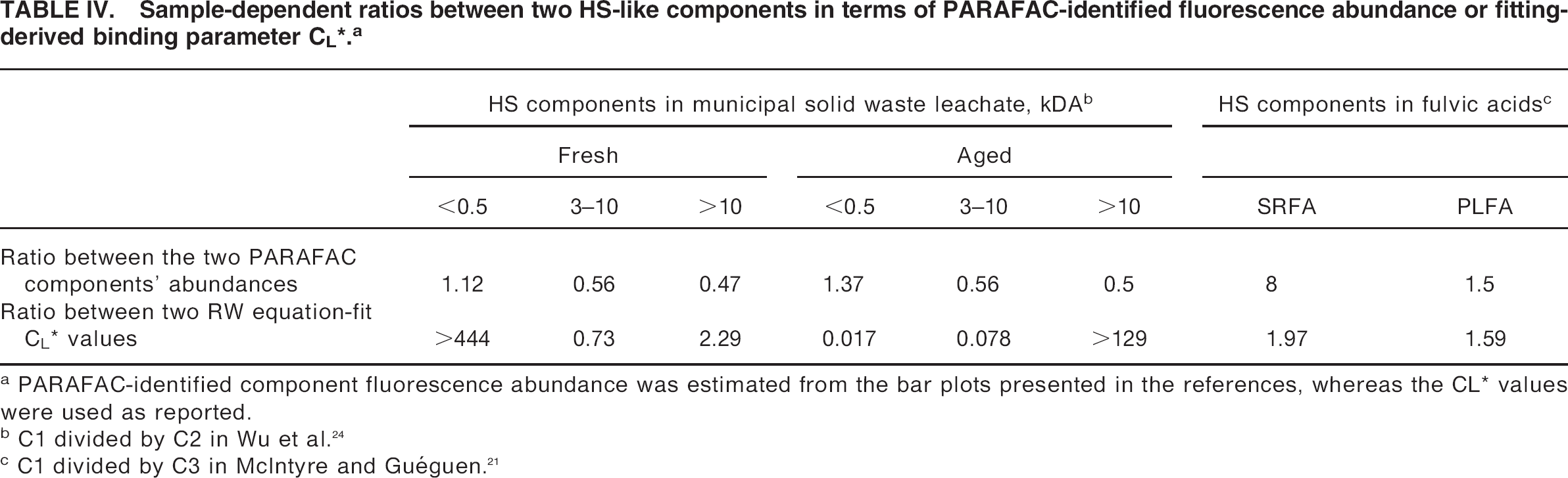
PARAFAC-identified component fluorescence abundance was estimated from the bar plots presented in the references, whereas the CL* values were used as reported.

C1 divided by C2 in Wu et al.²⁴

C1 divided by C3 in McIntyre and Guéguen.²¹

As shown in Table IV, the fluorescence ratios in the fresh waste were estimated to be 1.12, 0.56, and 0.47 for the size fraction of <500 Da, 3–10 kDa, and >10 kDa, respectively; these ratios shifted to ∼1.37, 0.56, and 0.5 in the aged waste. Accordingly, the C_L* ratios shifted from >444, 0.73, and 2.29 to 0.017, 0.078, and >129. The fluorescence ratios did not show a significant difference (p > 0.358, paired t-test) between the fresh and aged samples, whereas the C_L* ratios did (p < 0.01, paired t-test). It was evident that these two types of ratios did not show mutual coupling, indicating that the HS component fluorescence abundance was not directly linked to the model-recovered C_L*.

The other report was by McIntyre and Guéguen,²¹ in which two fulvic acids were isolated by the same procedures and then their fluorescences were decomposed by PARAFAC into the same set of components. As shown in Table IV, the fluorescence ratio of two HS-like components (C1 and C3 as termed in that study) shifted remarkably from 8 to 1.5 from one fulvic acid to another, whereas the C_L* ratios shifted slightly from 1.97 to 1.59.

DISCUSSION

In Fig. 1a, the curve became steeper with the decrease of C_A. This may be accounted for by the competitive binding of Cu²⁺ by organic molecule A, a competing process that “delayed” the depletion of [L] relative to the accumulation of [LCu]; a fixed ratio of I/I₀ ratio therefore was observed at higher C_Cu in the presence of higher C_A than in the presence of lower C_A. On the contrary, as shown in Fig. 1b, an opposite trend was observed in case 2, in which higher C_A led to steeper fluorescence–response curves, indicating a faster depletion of [L] relative to accumulation of [LM] than in case 1.

The discrepancy among the fluorescence–response curve shapes may be better accounted for by the different values of log K_VII in the two cases. In case 2, the formation constant (10¹²) of the mixed ligand complex formation was more than three orders of magnitude greater than that (10^8.9) in case 1; as such, the mixing binding reaction (Eq. 7) was presumably more efficient in case 2 than in case 1 for depleting [L] relative to [LCu]. Therefore, the differing shapes of the fluorescence–response curves clearly demonstrated that concentrations of competing binding ligands (e.g., A) relative to the target component (i.e., L) and mixed ligand binding constants jointly played a role in “tuning” fluorescence–response curves in experiments.

Although K* was operationally defined in such a way (see Supplemental Material) that precluded recovering the underlying true binding parameters K, log K* in case 1 was consistently smaller than but comparably close to the true value (i.e., log K = 5 for LCu; Table I). However, in case 2, data fitting in the case of C_A = 10 μM and C_A = 50 μM resulted in large log K* values of 6.21 ± 0.06 and 6.95 ± 0.02, respectively, all of which were remarkably higher than the theoretically true value of 5. Despite the incorrectly high values of log K*, all of the fitting was equally good (R² = 0.9971–1.0), implying that other binding parameters, e.g., C_L* or φ, would also be biased for compensation.

Extremely low values of fitting-derived C_L* were sometimes observed for experimental data in previous studies^18,23 that did not consider the values to be chemically feasible in relation to the acidic group content of the samples. The appearance of low C_L* remains poorly understood,^18,23 but it may be better understood via this simulation that implies that fitting-derived C_L* is prone to high variability, largely dependent on the solution composition and the C_Cu range used for the fitting. Therefore, appearance of low C_L* (e.g., as low as 6.72 μM, 32.8% lower than the theoretically true value of 10 μM in this study) is possible for real titration data.

Compared with log K* and C_L*, the parameter φ does not have direct environmental implications to metal binding and metal speciation and thus has rarely been evaluated for the data reliability. The simulation in this study implied that the reliability of reported φ values in the literature is problematic.

As clearly shown by the simulation study, R² is not a reliable indicator for the validity of the assumptions of RW equation. The fluorescence–response curve of target ligand L was well fit to the RW equation, although the investigated system did not meet the assumptions. The failure of R² as a reliable indicator was further substantiated by an additional simulation study (see Supplemental Material), in which the metal binding constants of the ligand L and A were set to differ by two orders of magnitude (Table S1) to reflect the fact that different binding sites could show large differences in binding constants.¹⁸ Moreover, the additional simulation study showed that the fluorescence–response curves (F/F0 vs. C_Cu) during the copper titration did not necessarily show monotonically decreasing slopes with increasing C_Cu, as indicated in the top panel (see C_A = 10 and 50 μM) of Fig. S1. Similar fluorescence–response curves were implicated in an early real experimental study on fluorometric titration¹⁸ and were more clearly presented in the experimental study by Mounier et al.,²² who used the PARAFAC approach to resolve spectrally overlapping components. The additional simulation study also showed that fitting the classical RW equation to such type of fluorescence–response curves resulted in incorrect binding parameters and relatively low R² values (Tables S2–S5). Presumably realizing the failure of the RW model in curve fitting, Mounier et al.²² turned to fit a given component curve to a summation of multibinding site present in the component. However, our simulation study indicated that the multibinding site model may not be necessarily invoked to account for such “curved” plots.

The failure of R² as a reliable indicator was also indicated by the re-evaluation of some real experimental data reported previously. The decoupling between the two type of ratios calculated either from fluorescence intensity or from fitting-derived C_L*, as revealed by the re-evaluation, presented an “independent” evidence (in addition to the simulation results) that a good fit (as denoted by high R²) to the RW equation did not necessarily lead to chemically consistent results. Restriction to two types of organic molecules greatly simplified the simulation. A higher number of organic molecules will lead to a larger number of chemical equilibria involving the formation of a mixed ligand organic Cu²⁺ complex, thereby presenting a mathematical challenge to compute C_Cu. Note that the “mixed” binding is not always considered in commercial speciation modeling software, e.g., WHAM7, which does not take into account the mixed binding of a metal by two different HS components (e.g., fulvic or humic acid). WHAM2 only considers metal binding by discrete binding sites (mono-, bi-, or tridentate sites) located on each component.³²

It is difficult in practice to know the types and number of the binding ligands (e.g., acetate) that exist in environmental samples but that do not fluorescence, thus they are undetectable by fluorescence techniques. Therefore, the mass balance of the cupric species across the binding sites (organic plus inorganic ligands) in a given sample is difficult to describe in terms of mathematical expressions. This generates a problem when using the RW equation to determination of metal binding parameters specific to HS components.

Alternatively, free Cu²⁺ concentration [Cu²⁺] can be readily monitored by an ion-selective electrode during the Cu²⁺ titration experiments.³³ Given direct knowledge of [Cu²⁺] at each titration step, determination of metal binding parameters specific to PARAFAC-identified HS components will become much easier, and this approach is worthy of further work. The potential of the combination of both spectroscopic and potentionmetric measurements has been implicated by Benedetti et al.,^34,35 who have used the combination of luminescence (not the fluorescence of the HS) of rare-earth elements (e.g., europium) and potentiometric measurements to determination of sorption of the elements to a given sorbent (e.g., α-Al₂O₃ or humic acid).

CONCLUSIONS

Taken together, the findings in this study proved that fitting with success (denoted by high R²) to the classical RW equation cannot be used alone to verify the validity of the 1:1 binding stoichiometry and single binding site assumption when studying metal binding by HS. Re-evaluation of literature data supported this conclusion by showing decoupling between fluorescence abundance of HS and fitting-derived total binding ligand abundance. Such decoupling was unable to be accounted for based on the above-mentioned assumptions. An alternative to the current titration approach may be a joint application of an ion-selective electrode, fluorometric titration, and PARAFAC modeling, as well as a proper data analysis strategy in which free metal ions can be directly measured rather than computed or modeled based on complicated mathematical equations that are usually not applicable to unknown environmental samples.

Footnotes

ACKNOWLEDGMENTS

This work was supported by the National Scientific Support Program of China and the intramural funding of State Key Laboratory of Environmental Criteria and Risk Assessment.

Notes

References

Rocker

Kisand

Scholz-Böttcher

Kneib

Lemke

Rullkötter

Simon

. “Differential Decomposition of Humic Acids by Marine and Estuarine Bacterial Communities at Varying Salinities”. Biogeochemistry. 2012. 111(1–3), 331–346.

Tipping

. Cation Binding by Humic Substances. Cambridge, UK: Cambridge University Press, 2002.

De Schamphelaere

K.A.

Janssen

C.R.

. “Effects of Dissolved Organic Carbon Concentration and Source, pH, and Water Hardness on Chronic Toxicity of Copper to Daphnia magna”. Environ. Toxicol. Chem. 2004. 23(5): 1115–1122.

Ryan

A.C.

Tomasso

J.R.

Klaine

S.J.

. “Influence of pH, Hardness, Dissolved Organic Carbon Concentration, and Dissolved Organic Matter Source on the Acute Toxicity of Copper to Daphnia magna in Soft Waters: Implications for the Biotic Ligand Model”. Environ. Toxicol. Chem. 2009. 28(8): 1663–1670.

Lamelas

Pinheiro

J.P.

Slaveykova

V.I.

. “Effect of Humic Acid on Cd(II), Cu(II), and Pb(II) Uptake by Freshwater Algae: Kinetic and Cell Wall Speciation Considerations”. Environ. Sci. Technol. 2009. 43(3): 730–735.

Di Toro

D.M.

Allen

H.E.

Bergman

H.L.

Meyer

J.S.

Paquin

P.R.

Santore

R.C.

. “Biotic Ligand Model of the Acute Toxicity of Metals. 1. Technical Basis”. Environ. Toxicol. Chem. 2001. 20(10): 2383–2396.

Paquin

Gorsuch

Apte

Batley

Bowles

Campbell

Delos

Di Toro

Dwyer

Galvez

Gensemer

R.W.

Goss

G.G.

Hostrand

Janssen

C.R.

McGreer

J.C.

Naddy

R.B.

Playle

R.C.

Santore

R.C.

Schneider

Stubblefield

W.A.

Wood

C.M.

K.B.

. “The Biotic Ligand Model: A Historical Overview”. Comp. Biochem. Physiol. C Toxicol. Pharmacol. 2002. 133(1–2), 3–35.

Chen

Zhu

Wilkinson

. “Validation of the Biotic Ligand Model in Metal Mixtures: Bioaccumulation of Lead and Copper”. Environ. Sci. Technol. 2010. 44(9): 3580–3586.

Peters

Merrington

De Schamphelaere

Delbeke

. “Regulatory Consideration of Bioavailability for Metals: Simplification of Input Parameters for the Chronic Copper Biotic Ligand Model”. Integr. Environ. Assess. Manage. 2011. 7(3): 437–444.

10.

Wood

C.M.

Al-Reasi

Smith

D.S.

. “The Two Faces of DOC”. Aquat. Toxicol. 2011. 105(3-4 Suppl): 3–8.

11.

Ryan

D.K.

Weber

J.H.

. “Fluorescence Quenching Titration for Determination of Complexing Capacities and Stability Constants of Fulvic Acid”. Anal. Chem. 1982. 54(6): 986–990.

12.

Ryan

D.K.

Thompson

C.P.

Weber

J.H.

. “Comparison of Mn2+, Co2+, and Cu2+ Binding to Fulvic Acid as Measured by Fluorescence Quenching”. Can. J. Chem. 1983. 61(7): 1505–1509.

13.

Ryan

D.K.

Weber

J.H.

. “Copper(II) Complexing Capacities of Natural Waters by Fluorescence Quenching”. Environ. Sci. Technol. 1982. 16(12): 866–872.

14.

Plaza

Brunetti

Senesi

Polo

. “Molecular and Quantitative Analysis of Metal Ion Binding to Humic Acids from Sewage Sludge and Sludge-Amended Soils by Fluorescence Spectroscopy”. Environ. Sci. Technol. 2006. 40(3): 917–923.

15.

Hernández

Plaza

Senesi

Polo

. “Detection of Copper(II) and Zinc(II) Binding to Humic Acids from Pig Slurry and Amended Soils by Fluorescence Spectroscopy”. Environ. Pollut. 2006. 143(2): 212–220.

16.

Hays

M.D.

Ryan

D.K.

Pennell

. “A Modified Multisite Stern–Volmer Equation for the Determination of Conditional Stability Constants and Ligand Concentrations of Soil Fulvic Acid with Metal Ions”. Anal. Chem. 2004. 76(3): 848–854.

17.

Hays

M.D.

Ryan

D.K.

Pennell

. “Multi-Wavelength Fluorescence-Quenching Model for Determination of Cu2+ Conditional Stability Constants and Ligand Concentrations of Fulvic Acid”. Appl. Spectrosc. 2003. 57(4): 454–460.

18.

Luster

Lloyd

Sposito

Fry

I.V.

. “Multi-Wavelength Molecular Fluorescence Spectrometry for Quantitative Characterization of Copper(II) and Aluminum(III) Complexation by Dissolved Organic Matter”. Environ. Sci. Technol. 1996. 30(5): 1565–1574.

19.

Ohno

Amirbahman

Bro

. “Parallel Factor Analysis of Excitation-Emission Matrix Fluorescence Spectra of Water Soluble Soil Organic Matter as Basis for the Determination of Conditional Metal Binding Parameters”. Environ. Sci. Technol. 2008. 42(1): 186–192.

20.

Zhang

P.J.

Shao

L.M.

. “Insight into the Heavy Metal Binding Potential of Dissolved Organic Matter in MSW Leachate Using EEM Quenching Combined with PARAFAC Analysis”. Water Res. 2011. 45(4): 1711–1719.

21.

McIntyre

Guéguen

. “Binding Interactions of Algal-Derived Dissolved Organic Matter with Metal Ions”. Chemosphere. 2013. 90(2): 620–626.

22.

Mounier

Zhao

Garnier

Redon

. “Copper Complexing Properties of Dissolved Organic Matter: PARAFAC Treatment of Fluorescence Quenching”. Biogeochemistry. 2011. 106(1): 107–116.

23.

Yamashita

Jaffe

. “Characterizing the Interactions Between Trace Metals and Dissolved Organic Matter Using Excitation–Emission Matrix and Parallel Factor Analysis”. Environ. Sci. Technol. 2008. 42(19): 7374–7379.

24.

Zhang

Shao

L.-M.

P.-J.

. “Fluorescent Characteristics and Metal Binding Properties of Individual Molecular Weight Fractions in Municipal Solid Waste Leachate”. Environ. Pollut. 2012. 162: 63–71.

25.

Berkovic

Einschlag

F.G.

Gonzalez

M.C.

Diez

R.P.

Martire

. “Evaluation of the Hg²⁺ Binding Potential of Fulvic Acids from Fluorescence Excitation–Emission Matrices”. Photochem. Photobiol. Sci. 2013. 12(2): 384–392.

26.

B.-D.

X.-S.

Wei

Z.-M.

Jiang

Y.-H.

Pan

H.-W.

Liu

H.-L.

. “The Composition and Mercury Complexation Characteristics of Dissolved Organic Matter in Landfill Leachates with Different Ages”. Ecotoxicol. Environ. Saf. 2012. 86: 227–232.

27.

Chen

Smith

Guéguen

. “Influence of Water Chemistry and Dissolved Organic Matter (DOM) Molecular Size on Copper and Mercury Binding Determined by Multiresponse Fluorescence Quenching”. Chemosphere. 2013. 92(4): 351–359.

28.

Cuss

C.W.

Guéguen

. “Impacts of Microbial Activity on the Optical and Copper-Binding Properties of Leaf-Litter Leachate”. Front. Microbiol. 2012. 3(166): doi:10.3389/fmicb.2012.00166.

29.

Masini

J.C.

. “Evaluation of Neglecting Electrostatic Interactions on the Determination and Characterization of the Ionizable Sites in Humic Substances”. Anal. Chim. Acta. 1993. 283(2): 803–810.

30.

Masini

J.C.

Abate

Lima

E.C.

Hahn

L.C.

Nakamura

M.S.

Lichtig

Nagatomy

H.R.

. “Comparison of Methodologies for Determination of Carboxylic and Phenolic Groups in Humic Acids”. Anal. Chim. Acta. 1998. 364(1–3), 223–233.

31.

Craven

A.M.

Aiken

G.R.

Ryan

J.N.

. “Copper(II) Binding by Dissolved Organic Matter: Importance of the Copper-to-Dissolved Organic Matter Ratio and Implications for the Biotic Ligand Model”. Environ. Sci. Technol. 2012. 46(18): 9948–9955.

32.

Lofts

Tipping

. “Assessing WHAM/Model VII Against Field Measurements of Free Metal Ion Concentrations: Model Performance and the Role of Uncertainty in Parameters and Inputs”. Environ. Chem. 2011. 8(5): 501–516.

33.

Cabaniss

S.E.

Shuman

M.S.

. “Combined Ion Selective Electrode and Fluorescence Quenching Detection for Copper-Dissolved Organic Matter Titrations”. Anal. Chem. 1986. 58(2): 398–401.

34.

Marang

Reiller

P.E.

Eidner

Kumke

M.U.

Benedetti

M.F.

. “Combining Spectroscopic and Potentiometric Approaches to Characterize Competitive Binding to Humic Substances”. Environ. Sci. Technol. 2008. 42(14): 5094–5098.

35.

Janot

Benedetti

M.F.

Reiller

P.E.

. “Colloidal α-Al2O3, Europium (III) and Humic Substances Interactions: A Macroscopic and Spectroscopic Study”. Environ. Sci. Technol. 2010. 45(8): 3224–3230.