The Impact of Customer Relationship Characteristics on Profitable Lifetime Duration

Abstract

The authors develop a framework that incorporates projected profitability of customers in the computation of lifetime duration. Furthermore, the authors identify factors under a manager's control that explain the variation in the profitable lifetime duration. They also compare other frameworks with the traditional methods such as the recency, frequency, and monetary value framework and past customer value and illustrate the superiority of the proposed framework. Finally, the authors develop several key implications that can be of value to decision makers in managing customer relationships.

Relationship marketing—the establishment and maintenance of long-term buyer–seller relationships—has profoundly influenced marketing theory and practice. Although the concept of relationship marketing is not new, organizations have recently started to focus on identifying and retaining long-term customers. Managers profess to do it in new and better ways every day (Fournier, Dobscha, and Mick 1998). Consider the following example: Before the 1990s, AT&T spent hundreds of millions of dollars per year trying to attract prospects to use its longdistance telephone service. Most prospects received similar offerings regardless of their specific needs. As a result, AT&T sent out millions of pieces of largely undifferentiated direct mail solicitations several times a year. In spite of this, less than 5% of the cases resulted in conversions, and even worse, many of these conversions were lost because of a high rate of churn (Grant and Schlesinger 1995). Today, AT&T analyzes its relationships with its customers and tracks in particular retention and termination characteristics. In 1994, through conscientious modeling efforts, AT&T attracted seven times as many customers as it did in 1990. Even more important, these customers have a different quality in their retention behavior. By analyzing the factors that drive retention, AT&T is much more efficient in (1) keeping customers who are at risk of defection and (2) better pinpointing the customers who are likely to be long-life customers in its acquisition campaigns (Li 1995). Thus, AT&T has embraced the core of relationship marketing: It is considerably more profitable to keep and satisfy existing customers than to renew a strongly churning customer base constantly.

To make relationship marketing work, marketers have started to adopt a customer management orientation, which emphasizes the importance of customer lifetime analysis, retention, and the dynamic nature of a person's customer–firm relationship over time (Kotler 1994). Given the discrepancies between concept and reality in relationship marketing, it is important to study the concept of customer management and customer lifetime for two reasons.

First, a better understanding is needed of the facets of a customer management orientation. For example, firms that adopt a customer management orientation need to consider how their activities impact their relationship with different customers. Anderson and Narus (1991) note that every industry is characterized by its own bandwidth of transactional and relational exchanges. Garbarino and Johnson (1999) show that short- and long-term–oriented customers differ in the factors that determine their future exchanges. Their results imply that a focus on customer satisfaction is likely to be effective for weak relational customers whereas marketing that is focused on building trust and commitment is more effective for the long-term relational group. Likewise, given the need to cater to specific customers rather than all possible customers (Dowling and Uncles 1997), an analysis of the relationship dynamics over time, such as lifetime activity patterns, becomes of paramount importance (Reichheld and Teal 1996). The results of Jap and Ganesan's (2000) study highlight the need to incorporate dynamic effects over the duration of the customer–firm relationship. Specifically, they find that the differential efficacy of various relationship management mechanisms changes over the course of a relationship.

The need for research in this domain also finds its expression in the Marketing Science Institute's research priorities. It has elevated the topic of customer management and the analysis of surrounding issues (e.g., value of loyalty, measuring lifetime value) to one of its capital research priorities.

Second, although the importance of an analysis of the dynamic customer–firm relationship is hardly disputed, empirical evidence is scarce. In particular, areas in need of research are noncontractual relationships—relationships between buyers and sellers that are not governed by a contract or membership. Specifically, how can the length of a customer's relationship with a firm be measured, given that the customer “never signs off?” How can the relationship be managed? Given that switching costs are low and customers choose to interact with firms at their own volition, this is a nontrivial question for noncontractual relationships. What is the strength and directional impact of the antecedent factors on the duration of a customer's relationship with a firm? If managers can understand the temporal dynamics involved in a customer's relationship with the firm, they can, for example, predict a customer's intention to leave the relationship. Consequently, they can spend marketing dollars more effectively either by not chasing customers “whose time has come” or by employing judicious marketing actions to save customers who are at risk. This issue gains added importance given Reinartz and Kumar's (2000) findings that both long-term and short-term customers can be profitable. Thus, it is imperative to develop a framework that incorporates customers’ projected profitability in the computation of lifetime duration. Furthermore, this framework should also identify factors under managers’ control that could increase the value of each customer for the firm. In other words, in the case of a noncontractual setting, it is a two-step process. First, we must measure lifetime duration that incorporates projected profits, and second, we must identify factors that can explain the variation in duration.

From a managerial standpoint, it would be desirable to know, at any given time, whether it would be profitable to mail a catalog or send a salesperson to a given customer. If it is profitable, the manager decides to mail the catalog or initiate a personal contract. On the basis of this decision framework, it is possible to compute lifetime durations for each customer. After profitable lifetime duration is obtained for each customer, managers are interested in knowing the factors or antecedents that drive the profitable lifetime duration. In response to this phenomenon, we present an integrated framework for measuring profitable customer lifetime duration and assessing antecedent factors. The key research objectives are to

•

Empirically measure lifetime duration for noncontractual customer–firm relationships, incorporating projected profits;

•

Demonstrate the superiority of our proposed framework by comparing it with the widely used recency, frequency, and monetary value (RFM) framework using the criterion of generated profits;

•

Understand the structure of profitable relationships and test the factors that affect a customer's profitable lifetime duration; and

•

Develop managerial implications for building and managing profitable relationship exchanges.

Our research takes place in the context of the direct marketing industry. This industry is important because in 1999, U.S. sales revenue attributable to direct marketing was estimated to reach close to $1.6 trillion. Approximately 15 million workers were employed throughout the U.S. economy as a result of direct marketing activity (Direct Marketing Association 1999). Specifically, we conducted our research for one of the leading general merchandise direct marketers (business-to-consumer [B-to-C] setting) in the United States. Furthermore, we validated the results with a customer sample from a high-technology firm (business-to-business [B-to-B] setting) selling computer hardware and software.

Review of Lifetime Duration Research

Several studies (Allenby, Leone, and Jen 1999; Bolton 1998; Dwyer 1997; Schmittlein and Peterson 1994) that are concerned with the empirical aspects of customer lifetime duration are somewhat limited because of the general lack of customer purchase history data. Given this historical lack of longitudinal customer information, researchers have predominantly focused on the retention construct (Crosby and Stephens 1987). Nevertheless, researchers have increasingly started to take a longitudinal perspective in their empirical work. Given the exploding managerial interest in how to manage the customer–firm relationship and the increasing availability of longitudinal customer databases, researchers have focused increasingly on empirically measuring and modeling a customer's relationship with a firm (Bolton 1998; Reinartz and Kumar 2000; Schmittlein and Peterson 1994). Although some researchers have analyzed lifetime behavior in contractual contexts (Allenby et al. 1999; Bolton 1998), findings from noncontractual settings (Reinartz and Kumar 2000; Schmittlein, Morrison, and Colombo 1987) require further investigation. In Table 1, we give a brief review of the academic literature concerned with customer lifetime duration as the focal construct. As can be seen from Table 1, research on customer lifetime duration and in particular profitable lifetime duration is scarce.

Table 1

Major Findings of Studies Concerned with Customer Lifetime Duration Modeling

Study	Nature of Study	Data	Highlights of Key Results/Remarks
Dwyer (1997)	• Description of the nature of customer lifetime and the procedures for lifetime estimation.	• n.a.	• Differentiation of always-a-share and lost-for-good customers. • Author proposes taxonomy for lifetime value estimation.
Crosby and Stephens (1987)	• Modeling satisfaction with service provider. • DV: satisfaction, retention.	• Life insurance	• Nonlapsing customers report higher satisfaction than lapsed customers (customers followed for 13 months only).
Schmittlein and Peterson (1994)	• Individual level analysis of purchase history.	• DV: probability of being alive.	• Office products in B-to-B context • Model can be used to infer the likelihood of a customer of being still active in a noncontractual context. • Model enables inferences about purchase and dropout process.
Li (1995)	• Proportional hazard model of customer tenure.	• Long-distance telephone service	• Model identifies variables (usage, marketing, and demographic variables) that affect length of customer subscription. • Build profile of customers with high and low lifetime.
Bolton (1998)	• Model of the duration of customer's relationship with firm (proportional hazard approach). • DV: customer tenure.	• Cellular phone service	• Customer satisfaction is related positively to subscription duration. • Prior cumulative satisfaction is weighted more heavily than recent satisfaction in decision to continue or not. • Because satisfaction plays a large role in explaining subscription duration, understanding and managing satisfaction becomes important.
Allenby, Leone, and Jen (1999)	• Bayes model of customer interpurchase time.	• Financial brokerage services	• The model allows managers to recognize when a customer is changing his or her purchase patterns (i.e., showing signs of defection). This prediction can be used managerially as a signal for the firm to employ some kind of intervention. • Individual customer level prediction.
Reinartz and Kumar (2000)	• Customer lifetime duration in a noncontractual setting.	• U.S. catalog retailer	• Both, long and short lifetime duration customers can be profitable to the firm. • “It is better to let go of some customers.”
Present Study	• Measuring profitable lifetime duration. • Explaining the variation in profitable lifetime duration.	• U.S. catalog retailer • High-tech B-to-B	• Model uses time-varying variables for explaining the impact of relationship characteristics on profitable lifetime duration. • Tells which customers to let go and when to let go of those customers.

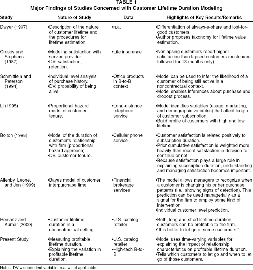
Notes: DV = dependent variable; n.a. = not applicable.

Specifically, the characteristics of a noncontractual setting, as explained previously, result in both long and short lifetime customers being profitable to the firm. Thus, there exists a need for conceptual and empirical exploration of the antecedent variables that can characterize profitable customers and not just the longer lifetime customers—thereby advancing our relationship management understanding.

A Dynamic Model of the Antecedents of Profitable Lifetime Duration

Reinartz and Kumar (2000) provide a descriptive model of the lifetime duration–profitability relationship. In this study, we attempt to build on their results and furnish new understanding in two key areas. First, the primary objective of our study is to show how an analysis of the antecedents of lifetime duration can help explain systematic differences in profitable customer lifetime duration. The goal is twofold: to better understand the structure of profitable relationships and to deduce implications for managers to better manage a customer's profitable tenure with the firm.

Second, our study builds on Reinartz and Kumar's (2000, p. 28) key finding that there exists “a substantial group of intrinsically short-lived customers, [and] it is necessary to identify this profitable yet short-lived group as early as possible and then stop chasing these customers” even though they may be contributing to the current sales. Their study does not tell the manager at what point the customers should not be pursued and which customers to let go. In this study, we attempt to provide managers with the framework to determine this information (based on their expected contribution margin [ECM]). Although a customer may be buying from the firm, it is in the firm's best interest to stop contacting that customer if the firm is losing money because of his or her transactions. In other words, our study offers a framework to identify the time periods beyond which customers may not be profitable. Niraj, Gupta, and Narasimhan (2001) also argue that estimating profitability at the individual level is important to distinguish the more profitable customers from the less profitable ones.

The modeling process of a customer's lifetime is contingent on a valid measurement framework that adequately describes the process of birth, purchase activity, and defection. The situation is far more difficult for noncontractual settings in which a customer purchases completely at his or her discretion. To our knowledge, no study has devised and tested a framework for measuring a customer's lifetime duration that considers projected profitability in a noncontractual context. Toward that end, we suggest a procedure for estimating the lifetime of customers and implement this procedure empirically.

The goal of this section is to conceptualize a model of profitable duration of the customer–firm relationship that is theoretically and empirically defendable. This model describes and analyzes how and why duration times differ systematically across customers. Thus, it is a customer-level analysis. An important aspect is that the customer's tendency to maintain a relationship is reflected in the evolutionary characteristics of his or her exchange with the firm over time (Ganesan 1994). Because our approach exploits longitudinal information obtained within customers, we refer to it as a dynamic model (see also Bolton 1998).

Figure 1 details the conceptual framework that centers on the focal construct of customers’ profitable lifetime duration. Profitable lifetime duration is conceptualized as a function of the characteristics of the relationship. In the hypotheses section, we discuss the exact nature of these influences. Figure 1 not only illustrates how our study differs from Reinartz and Kumar's (2000) study but also shows how our study incorporates their findings in the proposed framework, through the incorporation of revenues and cost in measuring lifetime duration. In summary, Reinartz and Kumar (2000) focus on the consequences of lifetime duration, whereas our study focuses on the antecedents of profitable lifetime duration. Managers understand the important consequences of both longer and shorter lifetime duration from Reinartz and Kumar's (2000) study. However, our study tells managers how to incorporate those findings in determining when to stop contacting customers.

Figure 1

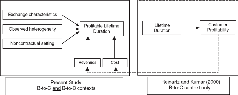
Conceptual Model of Profitable Customer Lifetime

The focus of our inquiry is on variables that determine the nature of the customer–firm exchange. Exchange characteristics encompass the variables that define and describe relationship activities in the broadest sense. First, the basic building blocks of any exchange can probably be characterized as the timing, scope, and depth of buying (Blattberg, Getz, and Thomas 2001; Neslin, Henderson, and Quelch 1985). For example, there is ample evidence in the marketing literature that behavioral exchange characteristics, such as past purchases, are strong predictors of future customer behavior (Dwyer 1997; Rossi, McCulloch, and Allenby 1996). In managerial practice, the key exchange characteristics reflect themselves in traditional customer scoring models that primarily take into account information on purchase frequency and purchase amount (Hughes 1996). In addition to these basic behavioral exchange variables, we consider other characteristics that are relevant to the growth or decline of a relationship. For example, this includes the communication between the firm and the customer in the form of not only marketing efforts but also signaling dissatisfaction (e.g., through product returns) or signaling commitment (e.g., through participation in loyalty programs).

Second, accounting for observed customer heterogeneity is clearly warranted. Observed customer heterogeneity is the degree to which customers differ on observed characteristics, for example, demographic or psychographic descriptives. It is important to consider these differences because demographic and psychographic indicators are most commonly used for segmentation purposes. For example, demographic information has been traditionally used in modeling customer response (Rossi, McCulloch, and Allenby 1996). Schmittlein and Peterson (1994) advocate the use of demographic information, though they point out that past purchase behavior (i.e., core exchange) generally outpredicts geodemographic information.

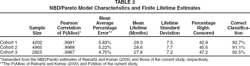
In general, the antecedents that are included in our model have received broad support in the relationship marketing literature (Sheth and Parvatiyar 1995). Because our effort deals with a single firm, we do not include competitive information. Specifically, we postulate that the profitable duration of a customer–firm relationship depends, differentially, on the exchange characteristics at time t and customer heterogeneity. Conceptually,

\begin{matrix} {Profitable lifetime duration}_{i} = f ({exchange characteristics}_{it}, \\ {customer heterogeneity}_{i}) . \end{matrix}

We capture the dynamic nature of the customer–firm relationship through the time varying nature of the independent variables. Although the impact of these variables has been studied in a response-modeling context (e.g., brand choice, interpurchase time), we are not aware of any study that assesses their impact on profitable lifetime duration (or on lifetime duration itself) in a noncontractual lifetime context.

Development of Hypotheses

In this section, we advance expectations about the effects of exchange characteristics on profitable lifetime duration. We form these expectations from theoretical and empirical knowledge from the relationship marketing paradigm, the social exchange paradigm, and loyalty and satisfaction-related research. Given the lack of research in the lifetime duration area in general and more so with respect to profitable lifetime duration, we also draw on the evidence available in related contexts (e.g., contractual settings, B-to-B settings) for developing the hypotheses.

When customers enter into commercial relationships, they seek to maximize their expected utility from the entirety of the exchange (Oliver and Winer 1987). The overall derived utility is a function of a multitude of factors, which varies across customers. However, in most cases, the substance of the expected utility is derived from the goods or services themselves.

Exchange Characteristics

Any given spending of a customer with the focal firm over time can be decomposed into three components: purchase frequency, purchase amount per incidence, and purchase composition (single or cross-category). This notion is also reflected in the generalized context of personal relationships that Kelley and Thibaut (1978) bring forward. They suggest that the interaction between two parties manifests itself in frequency of interaction, depth of interaction, and scope of interaction. Relationships intensify as exchange parties communicate more often, more deeply, and across a larger scope of issues. Thus, the argument brought forth from the social exchange domain suggests that as customers buy more, buy more frequently, and buy more across different categories, the relationship between them and the vendor becomes more durable. Oliver and Winer's (1987) utility framework supports the same logic and suggests that buyers who buy more, buy more frequently, and buy more across different categories have a better fit with the vendor's product and positioning and receive greater utility from it. Therefore, the relationship between the two parties is prolonged.

Purchase amount

Specifically, with respect to the purchase amount, Bendapudi and Berry (1997) argue that customers who have a higher commitment are also likely to seek greater relationship expansion and enhancement. There is empirical evidence in a contractual context that more satisfied customers have longer relationships with their service providers (Bolton 1998) and higher usage levels of services (Bolton and Lemon 1999). In a financial services context, Storbacka and Luukinen (1996) find that satisfaction is a function of relationship volume. Thus, a positive correlation can be expected between the relationship duration and the purchase volume. In other words, if a consumer devotes a larger share-of-wallet to a firm, the bond should be stronger. Consequently, we expect that long duration customers will, on average, have higher spending levels than those with a shorter duration.

H₁:

Profitable customer lifetime duration is positively related to the customer's spending level.

Cross-buying

Assuming that the firm offers products or services in different categories, consumers can purchase products in a focused manner or purchase across a variety of different categories. Cross-buying refers to the degree to which customers purchase products or services from a set of related or unrelated categories of the company. For example, in a general merchandise context, one customer might buy only women's shoes and formal wear, whereas another customer might purchase shoes, high-fashion, formal wear, sports wear, accessories, and textiles. In the latter case, the scope of interaction with the firm is rather broad, whereas in the former case, it is focused. With respect to scope of purchases (operationalized as cross-buying), there is little empirical evidence that links cross-buying with a customer's tenure. The few existing studies in the marketing domain have focused on the related, yet different, construct of cross selling (Chen et al. 1999; Drèze and Hoch 1998)—in particular on the direct effect of cross-selling on aggregate level outcomes, such as store sales or store choice. As compared with the cross-selling construct, far fewer studies deal with the cross-buying construct. According to Coughlan (1987), the benefits of one-stop shopping are the key drivers of customers engaging in cross-buying. What remains open in the literature is the effect of cross-buying on individual level outcomes such as customer retention or lifetime duration.

With respect to the impact of cross-buying on retention, our reasoning is as follows: In the context of contractual relations, customer retention is enhanced with cross-selling of multiple accounts or services as customer switching costs increase with multiple relationships (Srivastava and Shocker 1987). Although these switching costs do not exist in a noncontractual setting, customers benefit from knowing the retailers’ product range, the quality levels, and interaction processes (Reichheld and Teal 1996). Evidence for this contention also comes from the B-to-B context in which O'Neal and Bertrand (1991) find that customers who are in long-term relationships with their suppliers are characterized by a greater scope of the relationship (measured in terms of products supplied). Likewise, Hoch, Bradlow, and Wansink (1999) state that variety in offerings is viewed as the entry fee for maintaining future customer loyalty. Thus, it is believed that the consumers who consume from a variety of product lines are less prone to terminate the relationship.

H₂:

Profitable customer lifetime duration is positively related to the degree of cross-buying behavior that customers exhibit.

Focus of buying

In addition to the reasoning that lifetime duration increases as the degree of cross-buying increases, we can make a qualifying argument that is specific to a focused buyer.¹ For example, a customer may buy a specific item, such as jeans, on a regular basis from the retailer. Even if the customer does not buy any other product from the retailer, this would suggest something about that customer's desire to be a long lifetime customer. In contrast, we could argue that the wear-off of involvement with the firm and decrease in excitement about the product are greater when there is only limited interaction. Unlike the cross-buying hypothesis, this suggests a negative effect on lifetime duration. Because of the conflicting argument, we test the specific effect of much focused buying (i.e., one single department/category) versus nonfocused buying (i.e., anything more than a single department/category). Because of the previous reasoning, we do not posit a directional hypothesis. Instead, we test empirically for the effect.

We thank a reviewer for suggesting this possible effect.

H₃:

Profitable customer lifetime duration is related to focused buying behavior that customers exhibit.

Average interpurchase time (AIT)

The variable AIT has been used in the context of modeling purchase events—representing the frequency of interaction. The impact of a customer's AIT on lifetime duration can be argued from two perspectives. Lower AIT (i.e., more frequent purchasing given that the customer is alive) could be associated with longer lifetime because this would be an indicator of a strong relationship. Morgan and Hunt (1994) argue that to the extent that interactions are satisfactory, frequency of interactions might lead to greater trust, which should in turn lead to a longer relationship duration. This argument is in line with Kelley and Thibaut's (1978) social-exchange perspective and the person-perception literature (Neuberg and Fiske 1987), which suggests a stronger link between people when their interaction frequency increases. These arguments favor a negative relationship between AIT and lifetime (i.e., the longer a customer's interpurchase time, the shorter is his or her lifetime).

The previous argument purports that an extremely frequent buyer (low AIT) should have the longest lifetime. However, sustaining a high purchase frequency over a long life seems unreasonable, in particular for the general merchandise category. We might reasonably argue that there seems to be a lower limit for interpurchase time because purchases might occur on a regular basis. For example, it is unlikely that a customer purchases many different clothes at one time and then pauses to buy for several years. Rather, apparel is bought on a continuous, yet intermittent, cycle. This argument suggests that a long customer life is associated with an intermediate length of interpurchase time. Furthermore, if a customer buys with a short burst of high intensity (low AIT given the customer is alive), it would seem that this customer has a rather low lifetime because the customer has stocked up on items that should last for an extended time. In addition, sustaining low AIT over the long run seems rather improbable given finite income resources.

Both of these arguments seem to have merit, and the only way to reconcile them is by way of accommodating an inverse U-shaped relationship between AIT and lifetime duration. Consequently, we propose that AIT and lifetime duration are related in an inverse U-shaped fashion, whereby intermediate AIT is associated with the longest lifetime. We note that the construct AIT is not tantamount to modeling frequency of purchases. Although these two constructs are related, frequency is an absolute measure and AIT is a relative measure. Thus,

H₄:

Profitable customer lifetime duration is related to AIT in an inverse U-shaped manner, whereby intermediate AIT is associated with the longest profitable lifetime.

From a managerial standpoint, we note that the variables of purchase frequency and purchase amount are key input to traditional scoring models for customer evaluation. Furthermore, these variables are also reflected in customer valuation models, such as the customer equity model by Blattberg, Getz, and Thomas (2001)—thus adding face validity to the conceptualization of our exchange variables.

Returns

Merchandise returns pose a significant problem for direct marketers (Hess and Mayhew 1997). It is suggested that increasing returns are associated with increasing dissatisfaction. Customers return merchandise because they are dissatisfied with one or more attributes of the product, such as quality, fit, or performance. This is particularly true in the direct marketing context, in which the evaluation of the product attributes cannot be performed directly, but only through reading the catalogs or the product descriptions over the Internet. If we accept an inverse relationship of proportion of returns and overall satisfaction, then we would deduce that high returns should also be associated with shorter lifetimes. There is conceptual and empirical evidence that cumulative satisfaction/dissatisfaction leads to higher/lower repurchase intentions (Anderson and Sullivan 1993) and that cumulative satisfaction is associated with longer lifetimes for a long-distance telephone service (Bolton 1998). However, Gruen (1995) notes that though research generally supports the link between dissatisfaction with a relationship and the propensity to leave that relationship, the link is weak at best. Nevertheless, if return behavior is evidence of dissatisfaction with the firm's merchandise, we would consequently argue for lower lifetime duration expectations for those customers who return proportionally more.

H₅:

Profitable customer lifetime duration is inversely related to the proportion of merchandise that customers return.

Loyalty instrument

Another variable that should have an impact on characteristics of the exchange is whether a customer subscribes to the loyalty instrument of the focal firm. The firm's loyalty instrument takes the form of a charge card for which customers can sign up. The charge card itself is a free service, though customers must go through a credit rating process. Furthermore, the charge card is vendor specific, thus it cannot be used at other stores. Although the charge card performs a function in itself (i.e., the payment function), from a theoretical perspective, ownership of a charge card can also be explained through the process of identification with the firm. This is because customers must spend additional efforts (e.g., application process, danger of rejection due to credit rating) to obtain the card. Given that purchase payments can be managed in multiple ways (e.g., credit card, check), the identification with the focal firm seems to be a substantive driver behind the ownership. Customers typically use the firm's loyalty instrument to receive some discount or accumulate points to redeem in the future. Given that card programs come at a significant cost, it seems imperative to assess their impact on relevant outcomes, one of which is customer tenure. The empirical evidence is quite mixed. Hartnett (1997) points out that store card programs are associated with increased sales in the form of higher average purchases and more frequent store visits. However, Sharp and Sharp (1997) and Crié, Meyer-Waarden, and Benavent (2000) find that loyalty programs in the grocery context have only a marginal effect on customer loyalty. In this study, we are not examining a classical loyalty program in which customers can redeem loyalty incentives. Consequently, there is no question whether the loyalty program creates loyalty toward the firm or program itself. We believe that it is the identification with the firm that drives adoption of the card. As such, this suggests a positive association between company-specific credit card ownership and lifetime duration. Besides the directional impact, it will also be useful to assess the size of the impact of card ownership on lifetime duration.

H₆:

Profitable customer lifetime duration is positively related to the customer's ownership of the company's loyalty instrument.

Mailings

In general merchandise direct marketing, the prime communication channel from firm to customer is the product catalog. In our case, the company engages in virtually no broadcast advertising, but relies almost exclusively on list rental and mail solicitation (e.g., promotions, catalogs). Therefore, the inclusion of mailing efforts into the model represents the major marketing component of the firm. An impediment to the straightforward inclusion of mailing efforts into the model is the inherent complexity of the simultaneous nature of marketing effort and customer response probability. This simultaneity in modeling response is caused through the application of customer scoring models, and the problem is widely known in the direct marketing field (Dwyer 1997). Nevertheless, we suggest that the effect of mailings should be taken into account. We do this by including the company's marketing effort as a lagged variable in the model. Therefore, we avoid causal misinterpretation of the effect of marketing efforts by removing the associated variance from the model. Similar to Bult and Wansbeek (1995), we operationalize mailings by the number of efforts/mail pieces sent to the customer. Overall, we expect a positive impact of mailings on a customer's lifetime duration.

H₇:

Profitable customer lifetime duration is positively related to the number of mailing efforts of the company.

Product category

We classify general merchandise products customarily into two broad categories—soft goods and hard goods. Soft goods include all types of apparel, clothes, and fashion. Hard goods comprise all nonfashion items, such as small electronics, houseware, kitchenware, gifts, and the like. To control for potential systematic lifetime differences associated with one or the other category, we introduce a dummy variable that characterizes a buyer as either a soft good or a hard good purchaser depending on his or her majority of purchases. Because the variable is introduced for control purposes only, no directional hypothesis is advanced.

Customer Heterogeneity

Demographic variables that capture observed customer heterogeneity have been used consistently in response modeling. The main motivation to include these variables is for statistical control purposes and potential segmentation purposes. According to Zeithaml (2000), firms need to characterize attractive segments into identifiable and measurable groups of customers. There exists ample empirical evidence that demographic variables can be related significantly to the response variable (e.g., sales, choice, interpurchase time), yet the portion of explained variation is somewhat low (Rossi, McCulloch, and Allenby 1996). In this context, we specifically examine heterogeneity in terms of the customer's spatial location, age, and income.

Spatial location of consumer

The maintenance of relationships can be argued from a (customer's) economic perspective. It has been shown that the continuance of a relationship is a function of the cost and the benefits that accrue from the relation. Thus, this view emphasizes switching cost and dependence as key drivers of relationship maintenance (Dwyer, Schurr, and Oh 1987; Williamson 1975). For example, for grocery purchases, it has been consistently shown that store location is a key driver of store choice (Craig, Gosh, and McLafferty 1984). Thus, from an economic perspective, if a more expensive store is conveniently located to the buyer's location, ceteris paribus, the customer might still establish a relationship with that store because the customer minimizes overall cost (purchasing plus travel cost). Similarly, in our case, we expect that customers in rural areas, which are characterized by a lower population density, have fewer options in choosing their most preferred store. Fewer store options in the customer's local environment will translate, ceteris paribus, into a higher level of mail-order shopping. Consequently, because of the cost minimization argument, we expect a higher proportion of long lifetime customers to live in low-density areas than high-density areas (e.g., cities).

H₈:

Profitable customer lifetime duration is higher for customers living in areas with lower population density.

Age and income

Age and income are used as individual level control factors. We do not propose directional hypotheses for the age variable because of a lack of an appropriate theory. However, we posit a directional hypothesis for income. High-income households have high opportunity costs of time. They tend to substitute time by buying goods that will save time and are willing to pay for the added convenience. Therefore, high-income households tend to spend more money for the same bundle of products than low-income households. In general, customers with higher incomes are less susceptible to higher prices (Kumar and Karande 2000) and are expected to continue buying from the firm for the added convenience. Thus,

H₉:

Profitable customer lifetime duration is positively related to customers’ income.

Research Methodology

The data (B-to-C setting) for our study are the same as the data used by Reinartz and Kumar (2000). The use of the same data set is critical because we are trying to evaluate whether the findings from Reinartz and Kumar's (2000) study can be implemented successfully to determine which customers to let go of and when to let go of them. In addition to the two cohorts used in Reinartz and Kumar's (2000) study, an additional cohort of data was used from the data set provided to us. Thus, we can validate the results across three different sets of customers. Although the data are partially the same for both studies, the studies have different objectives. Furthermore, for this type of research, it is worthwhile to highlight that it is imperative to use cohort data (Parasuraman 1997; Reichheld and Teal 1996).

Database

We used data from a U.S. general merchandise catalog retailer for the empirical estimation in our article. The firm offers a broad assortment of products year round (e.g., apparel, gift items, decorative items, small electronics, kitchenware). We do not disclose the name of the company for reasons of maintaining confidentiality per the agreement. We describe the data here for the purpose of clarity and continuity. For this study, we recorded data that cover a three-year window on a daily basis. The database for the three cohorts consists of a total number of observations of 11,992 households. We tracked the customers from their first purchase with the firm. These households have not been prior customers of the company (i.e., no left-censoring). The sample of households belongs to three different cohorts; the structure is depicted in Figure 2.

Figure 2

Database Structure for B-to-C Setting

The customer–firm interaction of Cohort 1 households was tracked for a 36-month time period, the behavior of Cohort 2 households for a 35-month time period, and the behavior of Cohort 3 households for a 34-month time period. We randomly sampled households from all households that started in January, February, and March 1995, respectively. The number of purchases ranges from 1 to 46 across the sample with a median number of 5 purchases; the median interpurchase time is 117 days, and the median transaction amount is $91 for each purchase.

Estimation of P(Alive)

We replicated the estimation of the negative binomial distribution (NBD)/Pareto model used by Reinartz and Kumar (2000) to obtain the necessary parameter estimates for this study. In contrast to Reinartz and Kumar's (2000) study, we obtained the distribution parameters of the NBD/Pareto model for the entire sample through the maximum likelihood estimation (MLE; see details in the Technical Appendix). An added benefit of using MLE in this study is that we can compare the results with the method-of-moment estimates that are available from Reinartz and Kumar (2000).

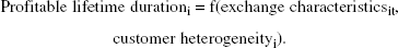
A key finding from the parameter estimation is that the method-of-moments and the MLE yield similar results (see Table 2). We also calculated the Pearson product moment correlation between the P(Alive) estimate from the MLE estimates and the P(Alive) estimates resulting from Reinartz and Kumar (2000). The correlation is greater than .99 for all three cohorts (Table 2), which also shows the convergent validity between the MLE and method-of-moment estimates. Given the convergent validity of the estimation method, we used the result of the NBD/Pareto model estimated by MLE. Specifically, we calculated the probability of being alive from month 4 to month 36 of the observation window. In Figure 3, we plot the resulting average probability for Cohorts 1 to 3. In the next section, we use P(Alive) and propose a rule for obtaining a finite lifetime estimate based on the expected future contributions of a customer. The procedure suggested subsequently is different from the one Reinartz and Kumar (2000) suggest. However, it integrates the knowledge gained from their study.

Table 2

NBD/Pareto Model Characteristics and Finite Lifetime Estimates

	Sample Size	Pearson Correlation of P(Alive)^*	Mean Average Percentage Error^**	Mean Lifetime (Months)	Lifetime Standard Deviation	Percentage Right-Censored	Correct Classification
Cohort 1	4202	.9981	5.83%	29.3	7.5	42.9	92.7%
Cohort 2	4965	.9988	5.22%	28.6	7.7	45.6	91.1%
Cohort 3	2825	.9987	4.75%	27.8	7.2	47.2	92.5%

Generated from the NBD/Pareto estimates of Reinartz and Kumar (2000) and those of the current study, respectively.

The P(Alive) of Reinartz and Kumar (2000) and P(Alive) of the current study.

Figure 3

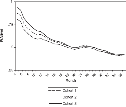
Average P(Alive) for Cohorts 1–3

Measuring Profitable Customer Lifetime Duration

Lifetime Duration Calculation

We suggest a four-step process for obtaining individual lifetime duration estimates that integrates projected profitability:

Calculate net present value (NPV) of ECM_it,

Decide relationship termination by comparing NPV of ECM_it with cost of mailing (i.e., if NPV of ECM_it < cost of next mailing_i, then terminate),

Calculate finite lifetime estimates, and

Conduct back-end performance analysis of the suggested procedure.

In the noncontractual setting, measuring lifetime duration becomes a nontrivial case. Here, customers are subject to “silent” attrition and firms can only infer when a customer has left the relationship. For example, even though a customer makes no purchase for a much longer period than the AIT, he or she might still have some nonzero probability of purchasing again. This spirit is captured by the NBD/Pareto model that reflects the probability of the customer being alive, given his or her particular purchase history. However, even though a customer might have a small probability of being alive (and thus to potentially purchase), this might not justify investing in this customer, for all practical purposes. For example, in the direct mail context, firms must optimize their resource allocation across customers because mail is sent out to customers regularly. Therefore, given that customers reach a low activity level at some point, the firm must make a decision whether to let this customer go. This managerial viewpoint reflects the spirit of our suggested procedure. If we want to determine the factors that have an impact on the length of a customer's tenure with the firm, we must establish a finite lifetime estimate, which in turn critically depends on our capability to determine the “death event.” Therefore, we argue that our suggested procedure of converting the continuous customer-specific P(Alive) estimate into a customer-specific finite lifetime estimate is fully compatible with the managerial decision-making process of retaining customers in the database and, at the same time, is a necessary intermediate step for our key modeling effort (i.e., hazard model).

Having established the raison d'être for our process, the next question is how to determine the lifetime estimate. In this section, we show how the expected future income stream can be used to determine the cutoff for the computation of profitable lifetime duration.

Calculate NPV of ECM_it

Given the nature of our data (and the data structure in the direct marketing industry in general), managers can easily determine past purchase and spending activity for each customer. Likewise, managers can obtain an estimate of the P(alive) status using the NBD/Pareto model for both past and future periods. This enables us to establish the following decision rule: If the sum of the expected discounted future contribution margin is smaller than a currently planned marketing intervention, we can establish the death event for the customer (e.g., a managerial consequence would be to stop mailing to that customer, even though this is not our primary concern). More formally, we compute the estimated future contribution margin as

{NPV of ECM}_{it} = \sum_{n = t + 1}^{t + 18} P {(Alive)}_{in} \times {AMCM}_{it} {(\frac{1}{1 + r})}^{n},

(1)

where ECM_it is the estimated ECM for a given month t, AMCM_it is the average contribution margin in month t based on all prior purchases since birth (updated dynamically), r is the discount rate (15% on a yearly basis), i is the customer, t is the month in which NPV is estimated, n is the number of months beyond t, and P(Alive)_in is the probability that customer i is alive in month n.²

Note that AMCM_it is the unconditional expectation of the contribution margin in a future period. Because the contribution margin is not conditional on purchase incidence, it is calculated from past periods—averaging over both, purchase and nonpurchase periods. This approach is applicable when the goal is to calculate the NPV of all future contribution margins, as is the case in our situation. Another possibility would be to use the conditional contribution margin [E(CM|Buy)]. This approach is particularly suitable if the goal is to predict discrete purchase incidences and expenditures per incidence (e.g., whenever decision makers want to optimize time and degree of marketing intervention). However, this is not the goal of our study.

For example, the NPV of ECM for customer i in month 18 is calculated as follows: For each month and for each customer, we observe the total purchases made in dollars. Then, we multiply that purchase amount by .3 to reflect the gross margin. In other words, the cost of goods sold is accounted for, and what we have is gross profit. Next, we subtract the cost of actual marketing efforts (in this case, the cost of catalogs plus the mailing costs) to obtain the monthly contribution margin. If a decision is made at the end of month 18, we take the average (AMCM_i) of months 1 through 18 by summing up all the 18 contribution margins and dividing it by 18. If we are at the end of time period 36, we take the average (AMCM) of the previous 36 months’ contribution margins by summing up all the 36 contribution margins and dividing it by 36.

It is possible that a customer might exhibit certain upward or downward trends. Any trend becomes incorporated into the AMCM_t and will lead to an upward or downward shift for a given period t. Nevertheless, the more we move through time, the more this trend becomes dampened because we divide by a growing number of periods. We believe this is a fair description of the actual process in which individual purchases represent shocks to the system but in which stationarity is achieved over time—representing that customer's purchase process. Furthermore, we would expect, on average, a general downward trend in the AMCM_t over time because of the ubiquitous attrition effect.

Thus, the AMCM estimate is updated on a monthly basis—in other words, dynamically modeled and used as a baseline for future purchases (i.e., purchases between t and N). The past purchase level at time t is projected into the future and multiplied monthly with the predicted P(Alive) estimate. Thus, it contains endogenously the information about the mailing process as well. The future time horizon is limited to 18 months because the associated P(Alive) estimate becomes only marginally different from zero after 18 months. For example, according to the NBD/Pareto model, if a customer has not purchased in a long time, his or her probability of being alive is small. Because the predicted P(Alive) for the next 18 months will be even smaller, the NPV of the expected future contribution margin stream will be low. Thus, for a manager who must decide whether to invest in this customer (i.e., marketing intervention), chances are that this customer would not be deemed as a lucrative future customer, given the cost of mailing.

Is a formal model needed for our purpose in the first place? With the use of the proposed model, it is possible to predict the value of P(Alive) beyond the range of the data. The key contribution of the model is a decision rule that is based on an assessment of the future value of a customer. Based on an extrapolation of the two components, P(Alive) and AMCM_it, the model allows for the construction of a score (NPV of ECM). This score can be constructed at any given t without having any knowledge of future customer behavior. Thus, the model is clearly aligned with the managerial decision-making process.

Decide relationship termination

Formally, if NPV of ECM_it < cost of mailing, the firm would decide to terminate the relationship. Using this decision rule, we establish for every customer at what point he or she is subjected to the proposed termination policy. The decision rule incorporates the cost of mailings and an average flat contribution margin before mailings of 25%. We assume the discount rate to be 15%, which is in the range of what has been used by other researchers (e.g., Berger and Nasr 1998).

Calculate finite lifetime estimates

Based on the decision of relationship termination, the average lifetime across Cohort 1 is 29.3 months, across Cohort 2 is 28.6 months, and across Cohort 3 is 27.8 months (see Table 2). The consistency among the three cohorts is high. In all the cohorts, little more than 60% of the samples have a lifetime that is less than the observation window. Households clearly show variability in lifetime duration. This is evidenced through several factors such as the wide range between lowest and highest lifetime estimate, the standard deviation of the lifetime estimate, and the relatively small value of s in the NBD/Pareto model. Thus, we expect considerable scope for exploring the factors that have an impact on lifetime duration. Note that the lifetime duration estimates that incorporate projected profits are different from the estimates that do not incorporate profits (as in the Reinartz and Kumar [2000] study)

Conduct back-end performance analysis of the suggested procedure

We assessed the performance of the proposed method by performing three different tests. First, we assessed the quality of classification. For that purpose, we computed the proportion of customers who were misclassified, that is, whose relationships were declared as terminated, however, they purchased at least once after the lifetime event. We present the results in Table 2. Slightly more than 90% of the subjects were classified correctly within the three-year observation window. This result underlines the strength of the expected future contribution margin method.

Second, we compared the proposed method to the widely used RFM framework. Most direct marketing firms use the RFM method as a scoring method for customers and as a method for determining the mailing status of customers. Although classical RFM analysis is based on the customer's past purchase behavior along the three dimensions (Hughes 1996), we employed an advanced form of RFM scoring. Specifically, we used a regression analysis that contains the RFM variables as well as measures on cross-buying, depth of buying, and observed heterogeneity.³ Reinartz and Kumar (2000) do not provide any explicit comparison of their method with the RFM framework. We compared for two different time periods (18 and 30 months) the prediction of the NBD/Pareto model with the prediction resulting from the advanced RFM model. To make the results as comparable as possible, we assume that the firm spends a fixed mailing budget at each of the two dates. We sorted the sample according to the score, and given the fixed budget, we selected the top 30%, 50%, and 70%, respectively, of the customers for targeting. We then compared the total actual revenues generated for those customers from months 18 and 30, respectively, onwards, until the end of the observation window for the two methods.⁴ Table 3 shows that the proposed framework is superior to the RFM decision rule.

We thank a reviewer for suggesting the benchmark comparisons with the state-of-the-art RFM scoring and past customer value scoring.

The dependent variable for the RFM regression is the purchase amount in season 3 (i.e., month 13–18) and season 5 (i.e., month 25–30) to reflect two different time periods. The eight independent variables are measures for R (whether customer bought in previous season), F (number of times bought in previous season), M ($ purchases in previous season), cross-buying (in previous season), depth of buying (up to focal period), spatial location (population density), income, and age. After estimating the coefficients, customers are scored on their purchase behavior in the current season (i.e., season 3 and 5). The score is used to determine the selection.

For example, the proposed framework selection method yields revenues of $590,452 (see Table 3), whereas the corresponding result using the RFM method yields $442,534. In every case, the proposed framework selection approach yields higher revenues as compared with the RFM selection approach. Similarly, the proposed framework selection method yields a profit of $123,076, whereas the RFM selection method yields only $78,555. Although we obtained this result for 30% of customers selected from the top, the findings hold across the percentages of customers selected and across the different points in time. This finding is a remarkable support for the performance of the suggested framework, which uses the estimates of P(Alive) from the NBD/Pareto model in combination with the NPV of the ECM.

Third, we compared our method with another classification benchmark. We used cumulative past customer value as the variable to determine mailing status of the customer. The reason for choosing lifetime value is that managers expend significant efforts to retain high lifetime value customers. Similar to the RFM model, we compared for the same two time periods (18 and 30 months) the prediction of the NBD/Pareto model; the prediction resulted from the past customer value benchmark. We report the results in Table 3. The results show that our model, which is based on the dynamic NBD/Pareto model, performs better than the traditional methods. Thus, including the dynamics of the customer lifetime value evolution seems to hold considerable potential in terms of customer scoring and customer selection.

Table 3

Actual Revenues and Profits for the Selected Group of Customers Based on NBD/Pareto, RFM, and Past Customer Value Selection (Cohort 1)

Customer selection based on	Percentage of Cohort (Selected from Top)	Evaluation at 18 Months ($)	Evaluation at 30 Months ($)
NBD/Pareto with ECM	30 (n = 1260)	590,452 (123,076)	318,831 (62,991)
	50 (n = 2101)	756,321 (148,922)	361,125 (61,636)
	70 (n = 2941)	864,114 (165,735)	380,855 (60,305)
Advanced RFM	30 (n = 1260)	442,534 (78,555)	140,781 (27,582)
	50 (n = 2101)	599,100 (99,831)	186,267 (36,380)
	70 (n = 2941)	687,163 (110,244)	216,798 (42,839)
Past Customer Value	30 (n = 1260)	508,997 (86,820)	179,665 (35,916)
	50 (n = 2101)	648,772 (112,723)	210,860 (41,729)
	70 (n = 2941)	789,526 (138,124)	225,910 (44,738)

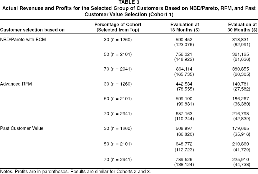
Notes: Profits are in parentheses. Results are similar for Cohorts 2 and 3.

The realized profits across the entire customer database could be of the order of millions of dollars, thereby enhancing the utility of our framework. Thus, although our suggested procedure is a theoretically sound procedure for the profitable lifetime calculation, it is also extremely well aligned with the actual managerial decision-making process. In and of itself, the result is useful to managers for optimizing mailing decisions.

In summary, we suggest a procedure for transforming the continuous NBD/Pareto outcome into a dichotomous “alive/dead” variable, which integrates projected profitability into a finite lifetime calculation. Recall that Reinartz and Kumar (2000) classify consumers with a greater than probability value of .5 for P(alive) as being alive and otherwise dead, without any consideration for profits. Our procedure improves on their heuristic. The NBD/Pareto framework could also be compared with a customer migration model (see, e.g., Dwyer 1997). Although a migration is based on average transition probabilities, our suggested framework allows for heterogeneity across customers. Even though the NBD/Pareto model might still be limited in capturing heterogeneity across the customer base, it appears to be an improvement over static approaches such as migration models.

Analysis

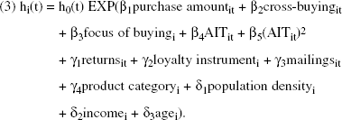
We used survival analysis for the analysis of profitable customer lifetime durations. It is the method of choice in dealing with duration data because it is well suited for the handling of censoring. We used the proportional hazard model, which assumes a parametric form for the effects of the explanatory variables but allows for an unspecified form for the underlying survivor function (Cox 1972). In the proportional hazard model, the hazard rate h_i(t) for individual i is assumed to take the following form:

h_{i} (t) = h_{0} (t) e^{x}_{it} β,

(2)

where h₀(t) is the baseline hazard rate and (x_itβ) is the impact of the independent variables.

We estimated the hazard model with the semiparametric partial likelihood method (Helsen and Schmittlein 1993). The partial likelihood considers the probability that a customer experiences the lifetime event, of all customers that are still considered alive. We used the PHREG procedure in SAS for the estimation; we handled ties using the exact likelihood instead of the more commonly used, yet less precise, Breslow approximation.

Variable Operationalization

The criterion variable is the household-specific estimate of profitable lifetime duration. Thus, there is only a single event associated with each household. We measured the length of the duration in months. The predictor variables in the model comprise both constant and time-varying variables. Time-varying variables may change during the course of a customer's lifetime spell, and they are measured and updated for each month. This procedure is exemplified with the returns variable. For example, a customer makes purchases worth $100 in month 1 and returns $20 worth of goods. Then, the customer does not purchase in month 2. Subsequently, the customer buys products for $60 in month 3 and returns nothing, and finally, in month 4, the customer buys products for $40 and returns 50%. Thus, the proportion of goods returned would be dynamically updated for every month such that the customer's returned proportion would be .2 for month 1 (because 20% is returned), .2 for month 2 (because nothing is bought), .125 for month 3 (because $20 is returned/$160 is purchased), and .2 for month 4 (because $40 is returned/$200 is purchased). We perform this updating for all time-varying variables, and this updating lies at the heart of the proportional hazard model. We do not provide means for the time-varying variables, because a simple mean statistic has limited value as a result of its averaging across time periods and individuals. (The detailed means report for every time period is available from the authors.)

The time-varying variable purchase amount_it enters the model as the monthly spending level ($). The time-varying variable cross-buying_it is operationalized as the number of different departments shopped in a given six-month period. There is a total of 90 different merchandise departments. The focus-of-buying variable is operationalized as a dummy variable. The percentage of customers who are coded as “1” (buying consistently in one department) is .04, .05, and .04 across the three cohorts. We measure the time-varying variable AIT_it in number of days between purchases. The AIT_it² is the square of the AIT_it variable. The return_it variable is the ratio of returned goods ($ value) to purchased goods ($ value). We operationalized the loyalty instrument_i variable as a dummy variable indicating ownership of the corporate charge card.

The proportion of customers holding a charge card is .39, .52, and .59 across the three cohorts. The effect of mailings_it is operationalized as a lagged finite exponential decay of past marketing efforts, similar to procedures in advertising–sales relationship literature. Because the merchandise changes on a continuous basis, the use of a finite decay period is more realistic than an infinite period. We measured the variable by the number of efforts or mail pieces sent to the customer. The dummy variable product category_i describes whether a buyer predominantly shops in hard goods or in soft goods. The proportion of customers buying predominantly hard goods is .50, .49, and .45 across the three cohorts. The variable population density enters the model as the absolute population number in a given two-digit zip code into the model. We obtained these numbers from the 2000 U.S. Census. The variable income_i comes from the firm's database and is coded on a scale from 1 to 7 (1 = “yearly income of lesser than $10,000” and 7 = “yearly income of more than $150,000”). The mean rating is 5.19, 4.88, and 5.01 across the three cohorts. Finally, we measured the age_i variable as the age of the individual in years, which was calculated from birth date information from the database. The mean rating is 34.4, 34.8, and 35.2 years across the three cohorts. We summarize all variables in Table 4.

Table 4

Variables for Profitable Lifetime Model

Dependent Variable	Measured as
Profitable Lifetime_i^*	Months
Independent Variables	Measured as	Hypothesized Directional Impact on Profitable Lifetime
Purchase amount_it^**	Monthly spending level ($), moving average over six-month period.	+
Cross-buying_it	Number of departments shopped in	(+)
Focus of buying_i	Dummy: 1 = buys consistently in single department only 0 = all other	Nondirectional hypothesis
AIT_it	Number of days	(+) Inverse U-shaped relationship for AIT and AIT²
(AIT_it)²	(Number of days)²	(-) Inverse U-shaped relationship for AIT and AIT²
Returns_it	Proportion of returns (of sales)	(-)
Loyalty instrument_i	Ownership of charge card. Dummy variable, 1 = owns card, 0 = no card	(+)
Mailings_it	Number of mailings sent in last six months (= 1 season) since current t, exponential decay, one month lag	(+)
Product category_i	1 = more then 50 % of purchases in soft goods, 0 = more then 50 % of purchases in hard goods	No directional hypothesis
Population density	Number of people in two-digit zip code	(-)
Income_i	Scale from 1 to 9 (1 is < $10,000 and 9 is > 150,000)	(+)
Age_i	Age of individual in years	No directional hypothesis

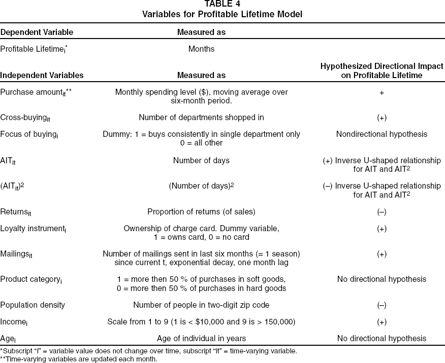
Subscript “i” = variable value does not change over time, subscript “it” = time-varying variable.

Time-varying variables are updated each month.

The complete model specification is given in Equation 3. The hazard of a lifetime event of a household i at time t is given as follows:

\begin{matrix} h_{i} (t) = & h_{0} (t) EXP (β_{1} {purchase amount}_{it} + β_{2} {cross-buying}_{it}) \\ + β_{3} {focus of buying}_{i} + β_{4} {AIT}_{it} + β_{5} {({AIT}_{it})}^{2} \\ + γ_{1} {returns}_{it} + γ_{2} {loyalty instrument}_{i} + γ_{3} {mailings}_{it} \\ + γ_{4} {product category}_{i} + δ_{1} {population density}_{i} \\ {+δ}_{2} {income}_{i} + δ_{3} {age}_{i}) . \end{matrix}

(3)

We estimated the model for each cohort in three steps to judge the incremental variance explained by the three models. First, we modeled the traditional key exchange variables (βs), second, we added the additional exchange variables (γs), and third, we entered the observed heterogeneity variables (γs).

Results

We report the results of the profitable lifetime duration model for the three cohorts in Table 5. The table contains the final model parameters, including an interaction term (returns x purchase amount), which was added post hoc.

Table 5

Coefficients (Standard Errors) for Profitable Lifetime Duration Model

		Cohort 1	Cohort 2	Cohort 3
Purchase amount_it	β₁	.0497^* (.00209)	.0360^* (.00212)	.0354^* (.00213)	.0486^* (.00186)	.0373^* (.00192)	.0364^* (.00192)	.0433^* (.00228)	.0341^* (.00240)	.0324^* (.00239)
Cross-buying_it	β₂	1.389^* (.0407)	1.293^* (.0417)	1.276^* (.0419)	1.226^* (.0327)	1.172^* (.0338)	1.154^* (.0340)	.970^* (.0346)	.908^* (.0356)	.912^* (.0360)
Focus of buying_i	β₃	-.315^* (.0647)	-.257^* (.0660)	-.270^* (.0662)	-.297^* (.0624)	-.306^* (.0630)	-.269^* (.0632)	-.289^* (.0841)	-.213^** (.0862)	-.177^** (.0865)
AIT_it	β₄	.0121^* (.000521)	.0133^* (.000521)	.0127^* (.000521)	.0146^* (.000515)	.0153^* (.000517)	.0147^* (.000519)	.0171^* (.000718)	.0178^* (.000724)	.0171^* (.000726)
(AIT_it)²	β₅	-8.994 E-6^* (6.276 E-7)	-9.880 E-6^* (5.900 E-7)	-9.487 E-6^* (5.892 E-7)	-.0000121^* (6.243 E-7)	-.0000123^* (6.013 E-7)	-.0000119^* (6.046 E-7)	-.0000151^* (8.912 E-7)	-.0000154^* (8.660 E-7)	-.0000147^* (8.747 E-7)
Returns_it	γ₁		-2.214^* (.222)	-2.050^* (.226)		-1.690^* (.214)	-1.557^* (.215)		1.323^* (.320)	1.323^* (.320)
Loyalty instrument_i	γ₂		.666^* (.0577)	.685^* (.0577)		.745^* (.0482)	.753^* (.0484)		.598^* (.0618)	.614^* (.0622)
Mailings_it	γ₃		.00552^* (.00153)	.00686^* (.00154)		.00628^* (.00148)	.00712^* (.00148)		.00610^* (.00224)	.00898^* (.00229)
Product category_i	γ₄		-.0278 (.0437)	-.0554 (.0438)		-.0360 (.0414)	-.0476 (.0414)		-.0422 (.0556)	-.0740 (.0558)
Returns x purchase amount_it	γ₅		.221^* (.0188)	.208^* (.0189)		.148^* (.0155)	.134^* (.0155)		.105^* (.0186)	.0985^* (.0183)
Population density_i	δ₁			-3.475 E-8^* (1.252 E-8)			2.23 E-8^** (1.196 E-8)			5.305 E-9 (1.584 E-8)
Income_i	δ₂			.124^* (.00863)			.111^* (.00805)			.133^* (.0104)
Age_i	δ₃			4.032 E-7 (4.668 E-6)			3.628 E-6 (4.123 E-6)			4.684 E-6 (5.446 E-6)
-2 Log-Likelihood R²		13728.6 .697	13337.7 .727	13126.8 .743	15.678.0 .684	15200.7 .719	15004.6 .730	9089.4 .652	8807.7 .672	8639.2 .693

Cohort 1

Cohort 2

Cohort 3

Independent Variables

Parameter

Model 1^†

Model 2

Model 3

Model 1

Model 2

Model 3

Model 1

Model 2

Model 3

Purchase amount_it

β₁

.0497^*

(.00209)

.0360^*

(.00212)

.0354^*

(.00213)

.0486^*

(.00186)

.0373^*

(.00192)

.0364^*

(.00192)

.0433^*

(.00228)

.0341^*

(.00240)

.0324^*

(.00239)

Cross-buying_it

β₂

1.389^*

(.0407)

1.293^*

(.0417)

1.276^*

(.0419)

1.226^*

(.0327)

1.172^*

(.0338)

1.154^*

(.0340)

.970^*

(.0346)

.908^*

(.0356)

.912^*

(.0360)

Focus of buying_i

β₃

-.315^*

(.0647)

-.257^*

(.0660)

-.270^*

(.0662)

-.297^*

(.0624)

-.306^*

(.0630)

-.269^*

(.0632)

-.289^*

(.0841)

-.213^**

(.0862)

-.177^**

(.0865)

AIT_it

β₄

.0121^*

(.000521)

.0133^*

(.000521)

.0127^*

(.000521)

.0146^*

(.000515)

.0153^*

(.000517)

.0147^*

(.000519)

.0171^*

(.000718)

.0178^*

(.000724)

.0171^*

(.000726)

(AIT_it)²

β₅

-8.994 E-6^*

(6.276 E-7)

-9.880 E-6^*

(5.900 E-7)

-9.487 E-6^*

(5.892 E-7)

-.0000121^*

(6.243 E-7)

-.0000123^*

(6.013 E-7)

-.0000119^*

(6.046 E-7)

-.0000151^*

(8.912 E-7)

-.0000154^*

(8.660 E-7)

-.0000147^*

(8.747 E-7)

Returns_it

γ₁

-2.214^*

(.222)

-2.050^*

(.226)

-1.690^*

(.214)

-1.557^*

(.215)

1.323^*

(.320)

1.323^*

(.320)

Loyalty instrument_i

γ₂

.666^*

(.0577)

.685^*

(.0577)

.745^*

(.0482)

.753^*

(.0484)

.598^*

(.0618)

.614^*

(.0622)

Mailings_it

γ₃

.00552^*

(.00153)

.00686^*

(.00154)

.00628^*

(.00148)

.00712^*

(.00148)

.00610^*

(.00224)

.00898^*

(.00229)

Product category_i

γ₄

-.0278

(.0437)

-.0554

(.0438)

-.0360

(.0414)

-.0476

(.0414)

-.0422

(.0556)

-.0740

(.0558)

Returns x purchase amount_it

γ₅

.221^*

(.0188)

.208^*

(.0189)

.148^*

(.0155)

.134^*

(.0155)

.105^*

(.0186)

.0985^*

(.0183)

Population density_i

δ₁

-3.475 E-8^*

(1.252 E-8)

2.23 E-8^**

(1.196 E-8)

5.305 E-9

(1.584 E-8)

Income_i

δ₂

.124^*

(.00863)

.111^*

(.00805)

.133^*

(.0104)

Age_i

δ₃

4.032 E-7

(4.668 E-6)

3.628 E-6

(4.123 E-6)

4.684 E-6

(5.446 E-6)

-2 Log-Likelihood R²

13728.6

.697

13337.7

.727

13126.8

.743

15.678.0

.684

15200.7

.719

15004.6

.730

9089.4

.652

8807.7

.672

8639.2

.693

Significant at p < .01.

Significant at p < .05.

†

Signs of coefficients have been reversed to reflect effect on lifetime.

The effective sample size for Cohort 1 is 3692 households, for Cohort 2 is 4323 households, and for Cohort 3 is 2491 households. We excluded 510 observations (12.1%), 642 observations (12.9%), and 334 observations (11.8%), respectively, because of missing values for the demographic variables. We rejected a chi-square likelihood ratio test of the hypothesis that the vector of independent variables is jointly equal to zero for all models (p < .0001).

As in all regression analyses, a measure analogous to R² is of interest as a measure of model performance. In a detailed study, Schemper and Stare (1996) show that there is not a single, easy to estimate, and useful measure for the proportional hazard model. In this context, we use the statistic proposed by Cox and Snell (1989) and endorsed by Magee (1990): R² = 1 – exp(–G²/n), where G² is the likelihood ratio chi-square statistic and n is the sample size. We give the R² estimates in Table 5 for all models. The increment in the proportion of variance explained in the more complex models is significant for all models and for all cohorts (p < .01).

Effects of Exchange Variables

Purchase amount

We hypothesized that the level of spending for merchandise (β₁) is positively related to profitable lifetime duration. We find support for this hypothesis across all three cohorts and across all three models (p < .01). Thus, H₁ is supported. Because of the strong association between these two measures, it is important to take information on amount of purchases into account when profitable lifetime duration is managed.⁵

Conceptually and empirically, it is important to include information on purchase amount in the duration model. Nevertheless, it could be argued that purchase amount is potentially correlated with AMCM. The reason it does not represent an endogeneity is because the purchase amount variable represents a revenue figure, whereas the AMCM variable represents a profit figure. It has been well established through previous research (Mulhern 1999; Niraj, Gupta, and Narasimhan 2001) that customer profitability varies tremendously through the simultaneous variation of revenues and cost per account. The second point of difference comes in through the measurement. Whereas purchase amount is measured as a six-month moving average, the AMCM is measured over the customer's lifetime. Although the time periods may have some overlap, the value of purchase amount that goes into the computation of contribution margin is different from the value of purchase amount used for the purchase amount measure. Empirically, we tested for the correlation between purchase amount and AMCM and found it to be moderate (.41–.52) across data sets. Thus, the magnitude of the correlation between purchase amount and AMCM does not pose a threat to the validity of the analysis. We thank a reviewer for bringing this issue to our attention.

We analyze the risk ratio to better understand the relative impact of this variable on the hazard of relationship termination. From a managerial standpoint, the risk ratio helps in gauging the impact of the drivers of profitable lifetime duration. We can interpret the risk ratio as the percent change in the hazard for each one-unit increase in the independent variable—controlling for all other independent variables. We calculated the risk ratio as {[exp(-β) – 1] x 100}. When applied to the purchase amount variable, a change of only $10 in the monthly spending results in a decrease in the hazard of termination of between 31 and 35%, depending on cohort.

Cross-buying

We argued that the degree of buying across departments (β₂) is positively related to profitable lifetime duration, because a broader scope of interaction constitutes a stronger relationship. This contention is supported for all models and for all cohorts in our model (p < .01). It appears that a long customer life is sustained by a higher degree of purchasing across departments. Given a certain income, people need a longer time to fill their needs if they purchase across the board rather than in a focused manner. When calculating the risk ratio for this variable, we found that purchases in an additional department are associated with a decreasing hazard of between 59.6 and 72.8%, depending on cohort. Thus, it seems to be desirable for the firm to induce customers to engage in cross-departmental shopping. Therefore, H₂ and H₃ are supported. This is an important finding because the effect of cross-buying on lifetime duration has not yet been documented.

Focus of buying

We did not advance a directional hypothesis with respect to focus of buying (β₃) because of conflicting arguments. The empirical test resulted in a negative relationship between focused buying behavior and lifetime duration. Thus, the result is in line with the results of the cross-buying construct—that is, broader buying is generally associated positively with an increase in lifetime duration.

AIT

We hypothesized that the AIT (β₄) is related to profitable customer lifetime duration in an inverse U-shaped fashion. That is, the longest profitable lifetime should be associated with intermediate interpurchase times. We tested for this relationship by introducing a nonlinear term AIT² (β₅). We find support for our hypothesis with both terms being significant at p < .01 and having the hypothesized sign (β₄ positive and β₅ negative). That is, lifetime tends to be shorter when interpurchase times are either short or long, and lifetime is longest with an intermediate value of AIT. Therefore, H₄ is supported.

Altogether, the impact of the core exchange variables on profitable lifetime duration is substantial. Between 65.2 and 69.7% of the variance is explained by this group of variables. Again, this demonstrates that the exchange variables dominate even in a noncontractual situation.

Returns

Regarding the proportion of returned goods (γ₁), we assumed a negative association of returns and profitable lifetime. That is, the higher the proportion of returned goods, the lower is the associated profitable lifetime duration. Our original results (not shown in Table 5) show that the effect was significant at p < .01 but had a positive sign for all three cohorts. Thus, our hypothesis that higher returns are a sign of greater dissatisfaction and lead to shorter lifetimes is not supported (H₅). A possible explanation for this outcome could be that customers who returned merchandise had a positive encounter with the firm's service representatives, which then might affect their future purchase behavior (Hirschman 1970).

Managers told us (on further inquiry) that heavy buyers tend to return proportionately more. A possible reason for this could be that these buyers are accustomed to the procedures of returning merchandise and that they are able to do it efficiently. Thus, it might be that these customers perceive the return process as part of the mail-order buying process. If this effect dominates, a positive relationship would be expected. Likewise, this would probably mean that as customers spend more with the firm, the effect should be stronger.⁶ To pursue this line of thought, we added, post hoc, an interaction between amount of purchases and the proportion of returns to the model. We present the final results including the interaction in Table 5. The interaction is significant for all three cohorts (p < .01).

We thank a reviewer for suggesting this interaction effect.

Thus, we find evidence for the conjecture that the degree of returns depends on the degree of spending. Thus, the positive impact on lifetime duration is greatest when the level of purchases and level of returns are high. Figure 4 depicts this situation graphically. Clark, Kaminski, and Rink (1992) show evidence of the impact of positively disconfirming complainants’ expectations to achieve (restore) satisfaction. Moreover, the impact of this response seems to be maintained over time. Therefore, we believe that proportionally higher returns might be an indication of this positive disconfirmation. For example, if the firm has a no-hassle return policy and customers have come to accept the technical return procedures, greater satisfaction with the exchange can result and therefore greater profitable lifetime duration. It would be desirable to have stated satisfaction measures at hand to add additional validity to our results. Similar empirical support for our finding comes from Kesler (1985) who states that Omaha Steaks, a mail-order supplier of high-quality meat, found higher profitability for the customers for whom it had quickly resolved complaints.

Figure 4

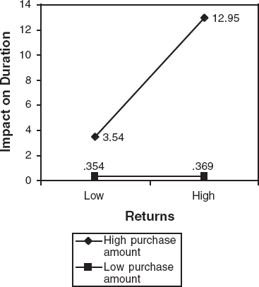
Interaction Between Proportion of Returns and Purchase Amount

Loyalty instrument

The loyalty instrument (γ₂) is significantly related to profitable lifetime duration (p < .01). According to our hypothesis, the use of the charge card as a loyalty instrument leads to a higher lifetime. Thus, in our sample, issuing a charge card appears to be successful as a loyalty instrument because it seems to be associated with longer customer lifetime. Thus, H₆ is supported. Note that the findings in the literature so far are not favorable in terms of loyalty instrument efficiency. However, in this case, it seems at least successful with respect to profitable lifetime duration. Nevertheless, we cannot make a statement about the cost-effectiveness of the program. This is in line with Day (2001) who suggests that though investments in relationship building programs result in relationship advantages, the effect on profits is far from clear. Although we find support for Day's first contention, his second proposition is much more difficult to test. In terms of magnitude of effect, the risk ratio analysis indicates that adopting the loyalty instrument is associated with a 45%–52% decrease in hazard of relationship termination—a substantive amount.

Mailings

We introduced the mailing variable (γ₃) as an important control variable specified as a lagged effect. Recall that mailings and sales are typically not independent in a direct marketing context. The hypothesized effect on lifetime duration is positive. We find a positive, significant effect (p < .01) for all three cohorts, thus our decision to control for the variable is correct. Therefore, H₇ is supported in that the mailing effort is significantly related to profitable customer lifetime duration.

Product category

We were concerned in our modeling effort that the choice of product category (γ₄) could have a systematic effect on a customer's lifetime. For example, it could be that durable goods (i.e., hard goods) have a potentially long lifetime, and thus there is little need for replacement, leading to a potentially shorter customer lifetime. However, this concern is not substantiated because the parameter γ₄ for the dummy variable is not significant (p >.1) for any cohort.

Effects of Observed Heterogeneity

Spatial location of customer

We argued that the spatial location is linked to a customer's tenure with a direct marketer (δ₁) such that the population density is inversely associated with customer lifetime duration. Our results confirm this hypothesis (H₈) for two of the three cohorts (p < .05), thus underlining the need (1) to account for observed heterogeneity in duration modeling and (2) to demonstrate support for the transaction- cost minimization argument.

Income and age

In terms of the two demographic variables income (δ₂) and age (δ₃), we find that age is not related to profitable lifetime duration (p > .05), but income is related (p < .01). Our model indicates that higher income is associated with longer lifetime. Thus, H₉ is supported. Overall, the information on observed customer heterogeneity adds explanatory power to the duration model, above and beyond the exchange variables.

Model Validation

The data for validating the proposed framework are obtained from a high-technology firm located in the United States. The organization sells computer-related products to both small and large businesses. The product range includes personal computers, printers, software, networking equipment, servers, storage, e-business applications, and so forth. The data cover an eight-year period from 1993 to 2000. Given the product category, the eight-year period gives multiple opportunities for the businesses to purchase from this firm repeatedly. From this database, we chose a cohort of customers such that their first purchase occurred in the first quarter of 1993. We tracked these customers from their first purchases for a period of eight years. These customers had not purchased anything from this firm before this date. This resulted in a sample size of 4128 businesses. The number of purchases ranges from 4 to 39 across the sample with a median number of 11 purchases; the median interpurchase time is 179 days, and the median transaction amount is $18,481 for each purchase. Unlike the catalog industry, in which customers are contacted through mailing the catalog, in this firm, businesses are contacted through tele-salespeople (i.e., salespeople contact the businesses over the telephone). The details on the cost of each contact and the frequency of contact are also available at the firm level.

We estimated the NBD/Pareto model parameters, as before, using the MLE procedure and computed estimates for P(Alive). We obtained the profitable lifetime duration estimates using the first three of the four steps described previously. We used the lifetime estimates in the calibration of the hazard model (see Equation 5). The majority of the variables in Equation 5 are common to both the B-to-C and the B-to-B settings. A few points of differences between these two settings are worth noting. We replaced the loyalty instrument variable with a dummy variable whether a line of credit was available or not. Similarly, we replaced the mailings variable with the number of contacts and operationalized the product category variable as hardware versus software. In terms of heterogeneity variables, we replaced the age and the income variables with the age of the firm and the average annual revenue of the firm.

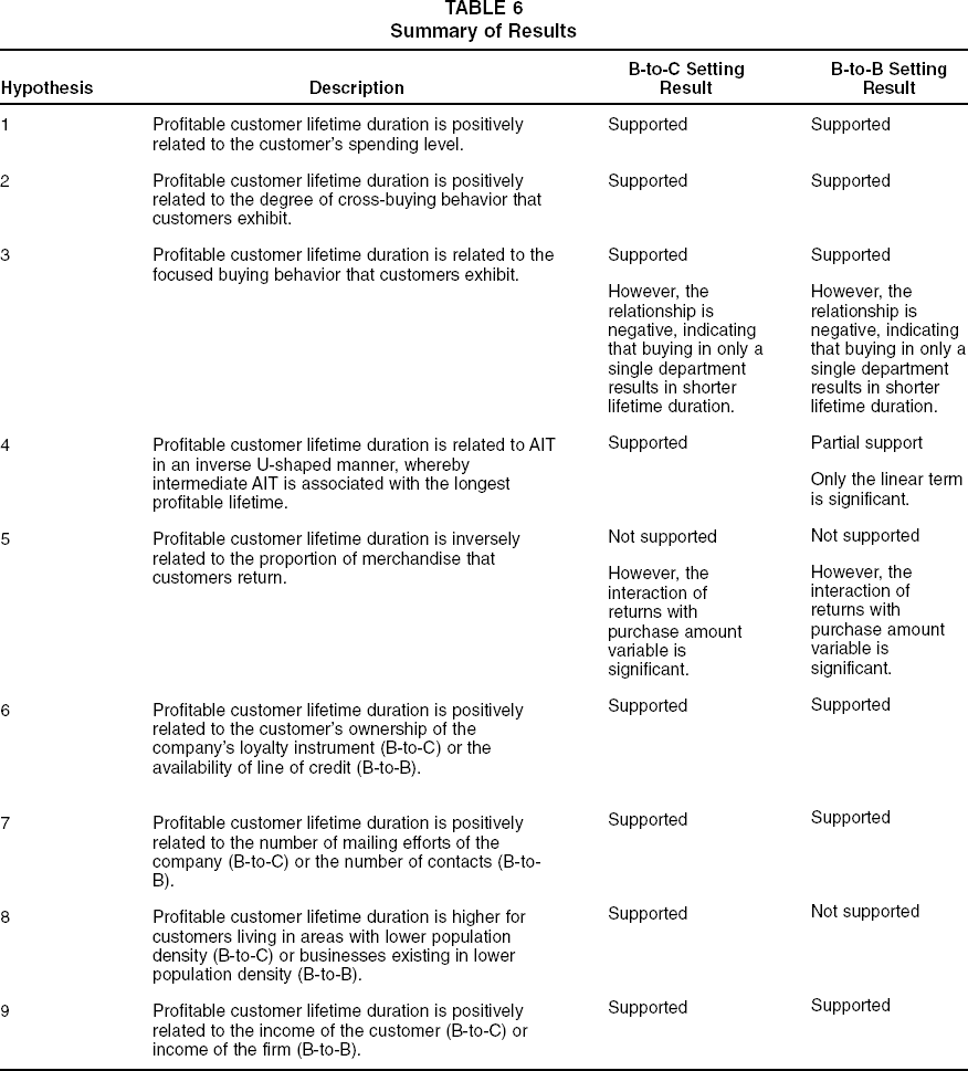
The results for the B-to-B case are similar to that of the B-to-C catalog industry. The most notable observations are that the variance explained by the key exchange, other exchange, and customer heterogeneity variables are 59%, 11%, and 4%, respectively. The businesses buying in only one department such as personal computer or networking equipment have shorter lifetime duration, firms with larger revenues have longer lifetime duration, and age of the firm was not significant. The AIT variable is significant but not the square of the AIT. However, the coefficient for AIT is negative, which indicates that shorter AIT is associated with longer profitable lifetime duration. It is possible that the range of the data is such that only a linear relationship is observed. Overall, there are more similarities than differences between the two settings (see Table 6). The findings indicate that the proposed theoretical framework holds across settings, providing evidence for generalizability of the results.

Table 6

Summary of Results

Hypothesis	Description	B-to-C Setting Result	B-to-B Setting Result
1	Profitable customer lifetime duration is positively related to the customer's spending level.	Supported	Supported
2	Profitable customer lifetime duration is positively related to the degree of cross-buying behavior that customers exhibit.	Supported	Supported
3	Profitable customer lifetime duration is related to the focused buying behavior that customers exhibit.	Supported However, the relationship is negative, indicating that buying in only a single department results in shorter lifetime duration.	Supported However, the relationship is negative, indicating that buying in only a single department results in shorter lifetime duration.
4	Profitable customer lifetime duration is related to AIT in an inverse U-shaped manner, whereby intermediate AIT is associated with the longest profitable lifetime.	Supported	Partial support Only the linear term is significant.
5	Profitable customer lifetime duration is inversely related to the proportion of merchandise that customers return.	Not supported However, the interaction of returns with purchase amount variable is significant.	Not supported However, the interaction of returns with purchase amount variable is significant.
6	Profitable customer lifetime duration is positively related to the customer's ownership of the company's loyalty instrument (B-to-C) or the availability of line of credit (B-to-B).	Supported	Supported
7	Profitable customer lifetime duration is positively related to the number of mailing efforts of the company (B-to-C) or the number of contacts (B-to-B).	Supported	Supported
8	Profitable customer lifetime duration is higher for customers living in areas with lower population density (B-to-C) or businesses existing in lower population density (B-to-B).	Supported	Not supported
9	Profitable customer lifetime duration is positively related to the income of the customer (B-to-C) or income of the firm (B-to-B).	Supported	Supported

Managerial Implications

The research objectives of this study are fourfold. First, we wanted to empirically measure customer lifetime duration that integrates projected profitability in a noncontractual setting. Second, we demonstrated the superiority of the proposed framework over the commonly used RFM framework and customer value framework. Third, we attempted to show how an analysis of certain factors (the antecedents) could help explain systematic differences in profitable customer lifetime duration, both in a B-to-C and a B-to-B setting. Fourth, we wanted to discuss how managers can use this knowledge in their decision making.

The use of a proportional hazard framework with finite lifetime estimates obtained from the combination of NBD/Pareto framework and expected NPV allows for a comprehensive and accurate analysis. We show that the model has a substantive explanatory power. Specifically, our analysis leads to the following implications:

The proportion of variance explained in the dependent variable rests to a large degree in the exchange variables. Thus, we find that the information that is quite easily available in the form of purchase history data is also strongly associated with customers’ profitable lifetime duration. In terms of actionable results, this is good news for the manager who can draw on an existing set of well-known variables to start managing profitable customer lifetime.

The B-to-C data support our assertion that the AIT is related in an inverse U-shaped fashion to profitable customer lifetime. Both long and short interpurchase times are seemingly associated with lower overall lifetime durations, however, for different reasons. The common view is that the higher the buying frequency, the “better” is the customer. This might be true if managers take a short-term cash-flow perspective. Traditional promotion-oriented marketing has clearly focused on this short-term response. However, what becomes clear here is that the evaluation of success depends much on the short- and long-term stance. In this context, the real impact of buying frequency is revealed only by examining the impact on lifetime duration. For many reasons (e.g., data availability, methodological issues), managers could not make a valid judgment about the long-term impact of relationship characteristics simply because it could not be measured. Given the available knowledge (i.e., about the short-term behavior and response), we implemented short-term actions. Our approach shows that, with respect to lifetime duration, it might mislead managers to regard high-frequency purchasers as the most attractive. The results show that if managers take a long-term (lifetime) perspective, it is the buyers with intermediate frequency that are most likely to be long duration customers.

Building on this reasoning, we conducted additional analyses on the drivers of this phenomenon. Specifically, why is it that buyers with a low AIT are not as profitable? In other words, is their profitability score low because of fewer purchase incidences or because of low expenditures given their buying frequency? It is the fewer purchase occasions (albeit high frequency) that distinguish this segment. Although their spending level is not much different from the overall average, these buyers are characterized by a sequence of fewer closely pulsed purchases. This behavior is consistent with that of a variety-seeker who does not stop buying because of dissatisfaction, but rather leaves the relationship because of the increased utility of variety.

A key implication is that managers are most likely successful in maximizing the customer's value to the firm if they fully understand the impact of specific relationship characteristics on short- and long-term success measures. Thus, our empirical finding is an important contribution to the managerial toolkit of actively managing customer equity. In terms of actionable results, this means that managers can now optimize their marketing efforts with respect to traditional short-term as well as new long-term objectives. There is no doubt that some traditional marketing practices will be questioned in the future. Concretely, the results enable managers to compare a customer's current interpurchase times with lifetime duration maximizing interpurchase times and adjust their solicitation plans accordingly. This should result in longer lifetime customers as well as higher customer satisfaction because the benefit to the customer is a communication policy, which is more consistent with his or her real needs. The insight in lifetime maximizing interpurchase times can and should be combined with other key long-term measures such as customer profitability.

The results enable managers to reassess their perceptions about the reasons for product returns. It was shown that longer lifetime customers have proportionally higher returns than shorter lifetime customers. The implications are twofold. First, it establishes that higher returns can be a symptom of a durable relationship and, thus, that the firm can use the information about return behavior to infer lifetime affinity. Clearly, the argument is only one way. There could be many reasons customers do not return what they bought—they are not dissatisfied, they are not accustomed to the return process, or they are dissatisfied and do not want to deal with the firm anymore. In this case, all the managers know is that the likelihood of being a long-term customer is lower. This knowledge might lead a manager to conduct more in-depth investigations such as customer feedback surveys to assess their state-of-the-relationship. If the customer returns merchandise, it shows that the customer does not shy away from the procedural hassle. Also, it gives the firm a further opportunity to interact and bond with the customer. This is also empirically supported by the findings of Bowman and Narayandas (2001) who find that loyal customers value how they have been treated (in a customer-initiated contact) more highly than whether they walked away from the contact having not received something valuable from the company. We are not suggesting that the firm should promote returns (as if it would make customers stay longer). However, managers should not necessarily be concerned about the relationship quality if returns from long duration customers are higher.

The second implication is that managing the cost component of the firm's return policy becomes highly critical. For example, a customer might order two different sizes of the same shirt with the purpose of trying on each and returning the one that fits worse. This behavior is more compatible with that of a regular, long lifetime client than that of a new client. If the client knows that the return process is hassle-free, he or she might as well use it. Thus, the managerial challenge is to satisfy the important client while containing operational cost.

The implication on the loyalty instrument policy is somewhat similar to the returns variable. From a response perspective, the loyalty instrument seems to be associated with longer lifetime customers, whichever way the causality works. By signing up to the card program, customers indicate that they are committed for the long haul. This is an important early signal for the manager, given that predictions on future lifetime duration are not easy to make. Thus, a manager can take this information and start treating this client as a likely long-term customer with all the relevant marketing-mix offers he or she deems appropriate. Besides the loyalty instrument's impact on exchange characteristics, cost management seems to be a major factor. Although an overall consensus on the effectiveness of loyalty programs is still not clear, the cost implications remain large (Day 2001).

Demographics matter not only with respect to purchase response and choice but also with respect to a long-term objective such as lifetime duration. In particular, we find that the higher the income and lower the population density, the greater is the likelihood of being a long-term customer. The overall incremental variance explained is relatively low, which is in line with other published research (Gupta 1991; Rossi, McCulloch, and Allenby 1996). However, the notion that an increasingly diversified and individualized population renders the value of demographics less useful (Sheth, Mittal, and Newman 1999) does not appear to hold. Thus, segmentation exercises based on demographic characteristics of the target customer groups still seem warranted. A significant advantage of the findings related to spatial location and demographics is regarding the acquisition of customers. If managers in the catalog industry are interested in recruiting new customers, a potential fertile group would be higher income people in lower population density areas.

Besides these substantive conclusions, our model provides the manager with a comprehensive general framework to analyze the role of antecedent factors in profitable customer lifetime duration. The time-varying nature of our model captures dynamic purchase behavior and is an advancement over many static approaches. Specifically, the model enables managers to dynamically update and quantify the direction and degree of impact on lifetime in a noncontractual context—something that has not been established so far. Thus, the model can be used as a tool for making profitability-based retention decisions. For example, as new data become available, managers can reestimate the model and identify customers who are likely to be profitable in the future but who stopped purchasing from the firm. Consequently, appropriate retention actions can then be taken to induce repeat purchases from these customers. In addition, the model enables managers to identify the point when a relationship turns unprofitable—even though these relationships might generate revenues. This is certainly advancement over other methodologies that focus on revenue as the key dependent variable. Thus, the model allows for selecting customers when lower levels of investments or no investment at all are more appropriate marketing decisions.

The firm that provided the B-to-B database actually collects data on share-of-wallet from the buying firms’ universe. This information can be combined with the profitable lifetime duration measure that is obtained in this study to create a 2 × 2 matrix as shown in Figure 5. The information in the figure should help managers deal with the existing customer. As indicated in Figure 5, if a customer belongs to the high share-of-wallet and high profitable lifetime duration, marketing strategies should aim at nurturing, defending, and retaining existing customers along with rewarding them for being such loyal customers. In contrast, if a customer belongs to a low–low segment in Figure 5, the focus could be on reducing marketing expense, considering divesting, or even outsourcing those customers for servicing by an outside agency that can operate on a percentage basis.

Figure 5

Firm's Strategy Based on Share-of-Wallet Versus Profitable Lifetime Duration

If a customer has high share-of-wallet but low profitable lifetime duration, the firm can use selective or optimal mailing/contract strategy to reduce cost, ensuring up-selling and cross-selling to increase the profit potential. Finally, if a customer's share-of-wallet is low but has high profitable lifetime duration, marketing strategies that focus on luring customer dollars from competition should be developed along with strategies for up-selling or cross-selling to encourage higher spending and lucrative loyalty programs. In summary, the findings in our study support the strategies suggested here.

In general, our analysis shows the relevance and importance of establishing customer relationship management capabilities. Our study shows that customers are heterogeneous on an important relationship characteristic—lifetime duration. We have documented how this heterogeneity can be measured and what the drivers of this heterogeneity are. Managers must take this knowledge and initiate systematic and appropriate supply-side responses. An appropriate firm response would be to develop customer management capabilities in situations in which customer behavior heterogeneity is present. Besides establishing the appropriate data recording, duration measurement, and profitability analysis capabilities, managers must develop systematic response procedures toward short- and long-life customers. For example, long-life customers can have access to more expensive but also more effective customer support. Alternatively, this can mean that short-life customers are subject to relationship enhancing activities. Regardless, of the specific marketing tactics, what is common to this kind of response is that firms must build their capabilities of handling an increasingly diverse customer base. In line with Day (2001), we believe that these are first and foremost strategic capabilities. Also, we believe that building these new customer management capabilities, which enable firms to establish competitive advantage, is one of the next frontiers of modern management. Given the importance of actively managing the customer base, our suggested framework provides an important tool toward this end.

Limitations and Suggestions for Further Research

It is important to point out the limitations of this study, some of which could be worthwhile topics for further research. Our empirical setting provides ways of testing previously unexplored issues in lifetime duration modeling, but it also limits the generalizability of the study. Although our data come from established companies in important industries, further empirical analyses in other noncontractual settings are necessary. Thus, although we implement a framework for analysis, other applications of this framework to cohort databases should yield fruitful insights.

Our procedure of calculating individual-level future contribution margin is based on a static extrapolation of a customer's ECM. Given the purpose of this study, and that the number of observations per household is limited, this measure seems adequate. Furthermore, we did not observe any trend in the purchase amount after the initial purchase in all of our datasets. Therefore, the use of an average measure is adequate. However, if enough purchase history observations are available, we could argue that incorporating any trend in purchase behavior is informative as well.

Another possible shortcoming could be the operationalization of the exchange construct. We use exclusively behavioral measures for operationalizing the duration antecedents. Although they provide for a strong and rich explanation, we could argue that attitudes such as satisfaction or attitudinal loyalty might interact with these behavioral constructs. However, we must leave this test to future inquiries because of the unavailability of appropriate data. Furthermore, if the correlation between the purchases amount variable and the AMCM is found to be high, the purchase amount variable can be removed from the analysis to avoid the problem of endogeneity.

In our calculation of a customer's NPV, we incorporate future marketing-mix costs implicitly by mirroring marketing-mix expenditures during the observation period. Although this is an important characteristic of the process, there are two aspects that are not fully considered. First, changing the amount of the marketing mix in the future might alter purchase behavior such that unprofitable customers become profitable (and vice versa). Second, our approach does not incorporate the quality of the marketing mix. For example, although our model might recommend letting a customer go, a different, better marketing mix for that customer would actually enable him or her to be profitable. Making a prediction conditional on marketing-mix expenditures would be an advancement over the current approach. We do not consider these conditional effects because both future marketing costs and purchase behavior are unknown. Also, Dwyer (1997) highlights the vexing difficulty of separating the two effects in a holdout scenario. Further research could focus on different patterns of expected marketing-mix costs in the holdout period to consider the consequences of varying the marketing-mix elements across customers.

From a technical perspective, the use of a two-step procedure of our model could be considered a limitation. However, the two-step modeling process is not particularly new to our problem but has been used and applied to many other marketing situations (e.g., Takada and Jain 1991). A well-known example is the new product diffusion context in which the first step consists of estimating the diffusion parameters and the second step regresses these parameters on a set of certain independent variables. Furthermore, although it has been shown that the benefit of integrating the two estimation procedures yields a gain in efficiency, this gain is typically small (Krishnamurthi and Raj 1988). The two-step approach also has an interesting precedent in a Grangerian sense in the econometrics literature. Our approach calculates and removes the effect of the recency of the last purchase in the NBD/Pareto model. Because the outcome variable P(Alive) has been prewhitened of the former variable's effect, the second step examines only the effect of what is left.

Footnotes

Technical Appendix

References

Allenby

Greg M.

, Leone

Robert P.

, and Jen

Lichung

, (1999), “A Dynamic Model of Purchase Timing with Application to Direct Marketing,” Journal of the American Statistical Association, 94(446), 365–74.

Anderson

Eugene W.

, and Sullivan

Mary

, (1993), “The Antecedents and Consequences of Customer Satisfaction for Firms,” Marketing Science, 12(2), 125–43.

Anderson

James

, and Narus

James A.

, (1991), “Partnering as a Focused Market Strategy,” California Management Review, 33(Spring), 95–113.

Bendapudi

Neeli

, and Berry

Leonard L.

, (1997), “Customers’ Motivation for Maintaining Relationships with Service Providers,” Journal of Retailing, 73(1) 15–37.

Berger

Paul D.

, and Nasr

Nada I.

, (1998), “Customer Lifetime Value: Marketing Models and Applications,” Journal of Interactive Marketing, 12(Winter), 17–30.

Blattberg

Robert C.

, Getz

Gary

, and Thomas

Jacquelyn S.

, (2001), Customer Equity: Building and Managing Relationships as Valuable Assets. Boston: Harvard Business School Press.

Bolton

Ruth N.

, (1998), “A Dynamic Model of the Duration of the Customer's Relationship with a Continuous Service Provider: The Role of Satisfaction,” Marketing Science, 17(1), 45–65.

Bolton

Ruth N.

, and Lemon

Katherine N.

, (1999), “A Dynamic Model of Customers’ Usage of Services: Usage as An Antecedent and Consequence of Satisfaction,” Journal of Marketing Research, 36(May), 171–86.

Bowman

Douglas

, and Narayandas

Das

, (2001), “Managing Customer-Initiated Contacts with Manufacturers: The Impact on Share-of-Category Requirements and Word-of-Mouth Behavior,” Journal of Marketing Research, 38(August), 281–97.

10.

Bult

Jan Roelf

, and Wansbeek

Tom

, (1995), “Optimal Selection for Direct Mail,” Marketing Science, 14(4), 378–94.

11.

Chen

Yuxin

, Hess

James D.

, Wilcox

Ronald T.

, and John Zhang

, (1999), “Accounting Profit Versus Marketing Profits: A Relevant Metric for Category Management,” Marketing Science, 18(3), 208–29.

12.

Clark

Gary L.

, Kaminski

Peter F.

, and Rink

David R.

, (1992), “Consumer Complaints: Advice on Companies Should Respond Based on an Empirical Study,” Journal of Consumer Marketing, 9(Summer), 5–14.

13.

Coughlan

Anne T.

, (1987), “Distribution Channel Choice in a Market With Complementary Goods,” International Journal of Research in Marketing, 4(2), 85–97.

14.

Cox

David R.

, (1972), “Regression Models and Life Tables,” Journal of the Royal Statistical Society, 34(2), 187–220.

15.

Cox

David R.

, and Snell

E. J.

, (1989), The Analysis of Binary Data, 2d ed. London: Chapman & Hall.

16.

Craig

C. Samuel

, Gosh

Avijit

, and Lafferty

Sara Mc

, (1984), “Models of Retail Location Process: A Review,” Journal of Retailing, 1, 5–36.

17.

Crié

Dominique

, Meyer-Waarden

Lars

, and Benavent

Christophe

, (2000), “Analysis of the Efficiency of Loyalty Programs,” working paper, Department of Marketing, University of Pau, France.

18.

Crosby

Lawrence

, and Stephens

Nancy

, (1987), “Effects of Relationship Marketing on Satisfaction, Retention, and Prices in the Life Insurance Market,” Journal of Marketing Research, 24(November), 404–11.

19.

Day

George S.

, (2001), “Capabilities for Forging Customer Relationships,” MSI Working Paper No. 00-118. Cambridge, MA: Marketing Science Institute.

20.

Direct Marketing Association (1999), Economic Impact: U.S. Direct Marketing Today/1998 Update. Chicago: The WEFA Group.

21.

Dowling

Grahame R.

, and Uncles

Mark

, (1997), “Do Customer Loyalty Programs Really Work?” Sloan Management Review, 38(Summer), 71–82.

22.

Drèze

Xavier

, and Hoch

Stephen

, (1998), “Exploiting the Installed Base Using Cross-Merchandising and Category Destination Programs,” International Journal of Research in Marketing, 15(December), 459–71.

23.

Dwyer

F. Robert

, (1997), “Customer Lifetime Valuation to Support Marketing Decision Making,” Journal of Direct Marketing, 11(Fall), 6–13.

24.

Dwyer

F. Robert

, Schurr

Paul H.

, and Oh

Sejo

, (1987), “Developing Buyer–Seller Relations,” Journal of Marketing, 51(April), 11–28.

25.

Fournier

Susan

, Dobscha

Susan

, and Mick

David G.

, (1998), “Preventing the Premature Death of Relationship Marketing,” Harvard Business Review, 76(January–February), 42–51.

26.

Ganesan

Shankar

, (1994), “Determinants of Long-Term Orientation in Buyer-Seller Relationships,” Journal of Marketing, 58(April), 1–19.

27.

Garbarino

Ellen

, and Johnson

Mark S.

, (1999), “The Different Roles of Satisfaction, Trust, and Commitment in Customer Relationships,” Journal of Marketing, 63(April), 70–87.

28.

Grant

Alan

, and Schlesinger

Leonard A.

, (1995), “Realize Your Customers’ Full Profit Potential,” Harvard Business Review, 73(September–October), 59–72.

29.

Gruen

Thomas

, (1995), “The Outcome Set of Relationship Marketing in Consumer Markets,” International Business Review, 4(4) 447–69.

30.

Gupta

Sunil

, (1991), “Stochastic Models of Interpurchase Time with Time-Dependent Covariates,” Journal of Marketing Research, 28(February), 1–15.

31.

Gupta

Sunil

, and Morrison

Donald

, (1991), “Estimating Heterogeneity in Consumers’ Purchase Rates,” Marketing Science, 10(3), 264–69.

32.

Hartnett

Michael

, (1997), “Private Label Credit Programs Enjoy Discount Store Boom,” Stores, 79(7), 44–46.

33.

Helsen

Kristiaan

, and Schmittlein

David C.

, (1993), “Analyzing Duration Times in Marketing: Evidence for the Effectiveness of Hazard Rate Models,” Marketing Science, 11(Fall), 395–414.

34.

Hess

James D.

, and Mayhew

Glenn

, (1997), “Modeling Merchandise Returns in Direct Marketing,” Journal of Direct Marketing, 11(2), 20–35.

35.

Hirschman

Albert O.

, (1970), Exit Loyalty and Voice. Cambridge, MA: Harvard University Press.

36.

Hoch

Stephen

, Bradlow

Eric T.

, and Wansink

Brian

, (1999), “The Variety of an Assortment,” Marketing Science, 18(4), 527.

37.

Hughes

Arthur M.

, (1996), The Complete Database Marketer, 2d ed. New York: McGraw-Hill.

38.

Jap

Sandy

, and Ganesan

Shankar

, (2000), “Control Mechanisms and the Relationship Lifecycle: Implications for Safeguarding Specific Investments and Developing Commitment,” Journal of Marketing Research, 27(May), 227–45.

39.

Kelley

Harold H.

, and Thibaut

John

, (1978), Interpersonal Relations: A Theory of Independence. New York: John Wiley & Sons.

40.

Kesler

Lori

, (1985), “Steak Company Welcomes Customer Grilling,” Advertising Age, 17(October), 36–37.

41.

Kotler

Philip

, (1994), Marketing Management. Upper Saddle River, NJ: Prentice Hall.

42.

Krishnamurthi

Lakshman

, and Raj

S.P.

, (1988), “A Model of Brand Choice and Purchase Quantity Price Sensitivities,” Marketing Science, 7(Winter), 1–20.

43.

Kumar

, and Karande

, (2000), “The Effect of Retail Store Environment on Retailer Performance,” Journal of Business Research, 49(August), 167–81.

44.

Shaomin

, (1995), “Survival Analysis,” Marketing Research, 7(Fall), 17–23.

45.

Magee

Lonnie

, (1990), “R² Measures Based on Wald and Likelihood Ratio Joint Significance Tests,” The American Statistician, 44(3), 250–53.

46.

Morgan

Robert M.

, and Hunt

Shelby D.

, (1994), “The Commitment–Trust Theory of Relationship Marketing,” Journal of Marketing, 58(July), 20–38.

47.

Morrison

Donald

, and Schmittlein

David C.

, (1981), “Predicting Future Random Events Based on Past Performance,” Management Science, 27(September), 1006–23.

48.

Neslin

Scott

, Henderson

Caroline

, and Quelch

John

, (1985), “Consumer Promotions and the Acceleration of Product Purchases,” Marketing Science, 4(2), 147–65.

49.

Neuberg

Steven L.

, and Fiske

Susan T.

, (1987), “Motivational Influences on Impression Formation: Outcome Dependency, Accuracy-Driven Attention, and Individuating Processes,” Journal of Personality and Social Psychology, 53(3), 431–44.

50.

Niraj

Rakesh

, Gupta

Mahendra

, and Narasimhan

Chakravarthi

, (2001), “Customer Profitability in a Supply Chain,” Journal of Marketing, 65(July), 1–16.

51.

Oliver

Richard

, and Winer

Russell S.

, (1987), “A Framework for the Formation and Structure of Consumer Expectations: Review and Propositions,” Journal of Economic Psychology, 8(4), 469–99.

52.

O'Neal

Charles

, and Bertrand

Kate

, (1991), “Developing a Winning J.I.T. Marketing Strategy,” Small Business Reports, 16(October), 68–71.

53.

Parasuraman

, (1997), “Reflections on Gaining Competitive Advantage Through Customer Value,” Journal of the Academy of Marketing Science, 25(2), 154–61.

54.

Reichheld

Frederick

, and Teal

Thomas

, (1996), The Loyalty Effect. Boston: Harvard Business School Press

55.

Reinartz

Werner J.

, and Kumar

, (2000), “On the Profitability of Long-Life Customers in a Noncontractual Setting: An Empirical Investigation and Implications for Marketing,” Journal of Marketing, 64 (October), 17–35.

56.

Rossi

Peter E.

, McCulloch

Robert

, and Allenby

Greg M.

, (1996), “The Value of Purchase History Data in Target Marketing,” Marketing Science, 15(4), 321–40.

57.

Schemper

Michael

, and Stare

Janez

, (1996), “Explained Variation in Survival Analysis,” Statistics in Medicine, 15(19), 1999–2012.

58.

Schmittlein

David C.

, Morrison

Donald G.

, and Colombo

Richard

, (1987), “Counting Your Customers: Who Are They and What Will They Do Next?” Management Science, 33(January), 1–24.

59.

Schmittlein

David C.

, Morrison

Donald G.

, and Colombo

Richard

, and Peterson

Robert A.

, (1994), “Customer Base Analysis: An Industrial Purchase Process Application,” Marketing Science, 13(1), 41–67.

60.

Sharp

Byron

, and Sharp

Anne

, (1997), “Loyalty Programs and Their Impact on Repeat-Purchase Loyalty Patterns,” International Journal of Research in Marketing, 14(5), 473–86.

61.

Sheth

Jagdish N.

, Mittal

Banwari

, and Newman

Bruce I.

, (1999), Customer Behavior. Fort Worth, TX: The Dryden Press.

62.

Sheth

Jagdish N.

, Mittal

Banwari

, and Newman

Bruce I.

, and Parvatiyar

Atul

, (1995), “Relationship in Consumer Markets: Antecedents and Consequences,” Journal of the Academy of Marketing Science, 23(4), 255–71.

63.

Srivastava

Rajendra

, and Shocker

Allan

, (1987), “Strategic Challenges in the Financial Services Industry,” in The Management of Strategic Change, Pettigrew

Andrew

, ed. Oxford, England: Basil Blackwell.

64.

Storbacka

, and Luukinen

, (1996), “Managing Customer Relationship Profitability—Case Swedbank,” in Proceedings from Banking and Insurance. Amsterdam: ESOMAR, 79–93.

65.

Takada

Hirokazu

, and Jain

Dipak

, (1991), “Cross-National Analysis of Diffusion of Consumer Durable Goods in Pacific Rim Countries,” Journal of Marketing, 55(April), 48–54.

66.

Williamson

Oliver E.

, (1975), Markets and Hierarchies. New York: The Free Press.

67.

Zeithaml

Valarie

, (2000), “Service Quality, Profitability, and the Economic Worth of Customers: What We Know and What We Need to Learn,” Journal of the Academy of Marketing Sciences, 28(1), 67–85.

The Impact of Customer Relationship Characteristics on Profitable Lifetime Duration

Abstract

Review of Lifetime Duration Research

A Dynamic Model of the Antecedents of Profitable Lifetime Duration

Development of Hypotheses

Exchange Characteristics

Purchase amount

Cross-buying

Focus of buying

Average interpurchase time (AIT)

Returns

Loyalty instrument

Mailings

Product category

Customer Heterogeneity

Spatial location of consumer

Age and income

Research Methodology

Database

Estimation of P(Alive)

Measuring Profitable Customer Lifetime Duration

Lifetime Duration Calculation

Calculate NPV of ECMit

Decide relationship termination

Calculate finite lifetime estimates

Conduct back-end performance analysis of the suggested procedure

Analysis

Variable Operationalization

Results

Effects of Exchange Variables

Purchase amount

Cross-buying

Focus of buying

AIT

Returns

Loyalty instrument

Mailings

Product category

Effects of Observed Heterogeneity

Spatial location of customer

Income and age

Model Validation

Managerial Implications

Limitations and Suggestions for Further Research

Footnotes

Technical Appendix

References

Calculate NPV of ECM_it