Expanding the Role of Marketing: From Customer Equity to Market Capitalization

Abstract

Can a marketer drive the stock price of the firm? Yes, it should be possible. Toward this endeavor, the authors develop a framework to link customer equity (CE) (as determined by the customer lifetime value metric) to market capitalization (MC) (as determined by the stock price of the firm). The authors test the framework in an empirical field experiment with two Fortune 1000 firms in the business-to-business and business-to-consumer contexts, respectively. The findings show that (1) a CE-based framework can reliably predict the MC of the firm and (2) marketing strategies directed at increasing the CE not only increase the stock price of the firm but also beat market expectations. Furthermore, the results indicate that the relationship between CE and MC is moderated by risk factors in the form of volatility and vulnerability of cash flows from customers. By accounting for these factors, the authors improve the association between CE and MC. The findings broaden the scope and role of marketing while reinforcing the importance of the marketer to any organization.

Keywords

shareholder value customer lifetime value market capitalization marketing accountability customer management

The world has become customer centric, in which firms are increasingly aligning their organizations around customers. Of late, this trend has gathered momentum with chief executive officers (CEOs) of many firms, who are expressing their intent to put customers at the top of the long list of issues they must focus on for growth (see The NYSE Euronext CEO Report 2008). These developments put marketing in the limelight—the function that best knows and understands the firm's customers. In such a scenario, the chief marketing officer (CMO) should be the most sought-after executive in the boardroom. In reality, however, the CMO is currently the most frequently fired C-level executive, with an average tenure of less than 24 months (see Welch 2004). More than half of all companies recently surveyed claimed that the marketing and the CEO agenda are not aligned in their organization (see ANA & Booz Allen Hamilton 2004). Clearly, there is a serious disconnect here. While an overwhelming majority of CEOs consider the marketing function of an organization “highly influential and strategic in the enterprise,” a large majority still believe that CMOs do not demonstrate adequate return on investment and thus fail to show the true potential of marketing (see The CMO Council Report 2007). Chief executive officers need CMOs to drive marketing strategies to obtain the maximum value from customer relationships. At the same time, the chief financial officer (CFO) needs to see the financial accountability of these strategies (Doyle 2000). To date, the marketing function across firms seems to be falling short on both imperatives. Rust, Lemon, and Zeithaml (2004) note that there is a perceived lack of marketing accountability, which has undermined marketing's credibility, threatened marketing's standing in the firm, and even threatened its existence as a distinct capability within the firm. The ominous premonition in Rust, Lemon, and Zeithaml's study resonates with the concerns raised in Webster, Malter, and Ganesan's (2003, p. 29) study, in which a CMO was quoted as saying, “Marketing has lost its seat at the (boardroom) table.” More damaging evidence comes from Nath and Mahajan's (2008) study, which analyzes a multi-industry sample of 167 firms and concludes that the CMO presence in top management teams has almost no impact on firm performance. Is marketing losing its clout? The answer lies in the marketers' ability to shake off the image of being tacticians rather than strategists capable of helping the CEO drive growth and profitability (Kumar 2004). This entails relating marketing performance to a higher-level financial metric that is of concern to the CEO. Toward this end, we propose a framework to link the outcome of marketing initiatives (as measured by customer equity [CE]) to the firm's market capitalization (MC) (as determined by the stock price of the firm). The intuition is that the stock price of the firm is based on the expected future cash flows of the firm. If cash flow is primarily generated from customers, an increase in CE (or cash flow from customers) should relate to an increase in MC (or the stock price of the firm).

Several managerially relevant questions emerge: Can CE really predict the MC of the firm? If so, can marketing strategies that increase CE also increase the stock price of the firm? In such a scenario, can the marketer predict and claim responsibility for the lift in the firm's stock price through appropriate marketing strategies? We attempt to answer these questions through an empirical application of our framework, which involves real-world data from a business-to-business (B2B) and a business-to-consumer (B2C) firm. Our results indicate that the CE metric can be used to reliably predict the average MC, or the stock price of the firm, within a maximum deviation range of 12%–13%. We further demonstrate how marketing managers can leverage appropriate marketing strategies not only to lift the stock price of the firm but also to beat market expectations. The results from our study hold implications for redefining the role of marketing as an organizational function that is capable of augmenting firm value through strategic customer management initiatives.

Theory

How is marketing related to firm value? Previous studies have investigated different ways of linking marketing activities and metrics to firm value. For example, researchers have shown relationships between satisfaction and firm value (e.g., Anderson, Fornell, and Mazvancheryl 2004; Fornell et al. 2006), brand and firm value (e.g., Kerin and Sethuraman 1998; Mizik and Jacobson 2008; Rao, Agarwal, and Dahloff 2004), advertisement and firm value (e.g., Joshi and Hanssens 2009), new product announcements and firm value (Sorescu, Shankar, and Kushwaha 2007), and so on (for a detailed review, see Srinivasan and Hanssens 2009). In this study, we focus our attention on how CE (as determined from customer lifetime value [CLV]) is related to firm value.

Understanding the CLV Concept

In recent years, the idea of managing customers on the basis of the CLV (or CE) metric has emerged as the most popular and efficient way of doing business. The appeal of the CLV metric lies in its ability to foster profitable customer relationship management (CRM) through appropriate marketing interventions (Villanueva and Hanssens 2007). Several approaches have been suggested to compute CLV (e.g., Fader, Hardie, and Lee 2005; Gupta, Lehmann, and Stuart 2004; Kumar, Luo, and Rao 2008; Lewis 2004; Reinartz and Kumar 2000; Rust, Lemon, and Zeithaml 2004; Venkatesan and Kumar 2004; Venkatesan, Kumar, and Bohling 2007). In essence, the CLV computation entails predicting the future cash flow from each customer by incorporating into a single equation the elements of revenue, expense, and customer behavior that drive customer profitability. This is then discounted by the cost of capital to arrive at the net present value of all future cash flows expected from a customer or the lifetime value of the customer. The sum total of lifetime value of all customers of the firm represents the CE of the firm. In other words, CLV is a disaggregate measure of customer profitability, and CE is an aggregate measure. Notably, CLV computation is conceptually analogous to the discounted cash flow method used in the accounting discipline to value firms. In such a scenario, can CLV be extended to relate to the MC of the firm?

Customer Value and Firm Value

Several researchers in the recent past have proposed strong theoretical arguments in favor of linking customer value to firm value, shareholder value, or the MC of the firm (Bauer, Hammerschmidt, and Braehler 2003; Berger et al. 2006; Srivastava, Shervani, and Fahey 1998). Consistent with these theoretical arguments, empirical studies have validated the claim that customer value can be used as a proxy for a firm's market value. For example, Kim, Mahajan, and Srivastava (1995) use the popular discounted cash flow method to estimate the value of business in the wireless communications industry. Gupta, Lehmann, and Stuart (2004) conduct an analysis across multiple firms to show that customer value can be as good as or a better method of firm valuation than traditional accounting. Rust, Lemon, and Zeithaml (2004) show that when they multiplied the average CLV of American Airlines' customer by the total number of airline passengers in the United States, the total customer value was more or less consistent with the MC of the firm. Libai, Muller, and Peres (2006) estimate the firm value from customer-based measures for five different companies and find that for four of the five, they could correctly estimate the firm value within an average deviation of 11.5%. Furthermore, prior studies have reported substantive findings that underscore the link between marketing and firm value. For example, Gupta, Lehmann, and Stuart (2004) quantify the impact on firm value resulting from improvement in retention, margin, and acquisition cost. Similarly, Rust, Lemon, and Zeithaml (2004) show how their CE framework can be applied to project return on investment from marketing expenditures. Not surprisingly, Wiesel, Skiera, and Villanueva (2008) extend a strong argument urging firms to report CE on their financial statements.

Collectively, these findings contribute to a growing and exciting stream of research that demonstrates the power of customer-based measures in shaping firm value. Our study proposes to advance these findings in several important ways. We take the CLV computation to the customer level rather than the industry level (Kim, Mahajan, and Srivastava 1995) or the firm level (Gupta, Lehmann, and Stuart 2004; Libai, Muller, and Peres 2006). By doing so, our study allows firms to differentiate the lifetime value across each customer and thus deploy differentiated marketing strategies that are relevant to each customer according to his or her lifetime value. For example, Gupta, Lehmann, and Stuart (2004) show that, on average, a 1% improvement in retention cost improves firm value by 5%. By implementing customer-level data, our study proposes to advance these findings by showing that a 1% improvement in retention cost can have a varying outcome on different customers ranging from a positive to a negative impact, depending on whether the 1% improvement in retention cost is directed toward highly profitable customers, less profitable customers, or unprofitable customers. Consequently, firms can be discretionary in terms of which specific customers to retain. This is imperative for firms that have a highly skewed distribution of lifetime value across customers. Indeed, most firms agree with the 80–20 Pareto principle (i.e., the top 20% of the customers usually provide close to 80% of the overall revenue and/or profits for the firm). This notion is consistent with the findings from recent empirical studies that have reported a highly skewed distribution of customer profitability (e.g., Kumar, Shah, and Venkatesan 2006; Rust, Lemon, and Zeithaml 2004). In such a scenario, marketing initiatives (e.g., improvement in retention) would be wasteful (or less efficient at best) if they were uniformly applied across all customers of the firm.

An important constituent of firm valuation is future cash flows. Studies on CLV to date have shown how to compute the value of future cash flows. However, they do not provide any insight into the nature of cash flows. Srivastava, Shervani, and Fahey (1998) contend that any firm's future cash flow is susceptible to inherent risks that can make the future revenue stream vulnerable and/or volatile, thus affecting firm valuation. In other words, given the same value of future cash flows for two firms, the firm with lower risk (i.e., lower volatility and vulnerability of future cash flows) can obtain a higher market valuation than the firm with higher risk. The vulnerability of cash flows is reduced when customer stickiness to the firm increases (as indicated by higher customer satisfaction, loyalty, and retention). Similarly, the volatility of cash flow is reduced when revenue streams from customers become more stable (Srivastava, Shervani, and Fahey 1998). We account for measures of volatility and vulnerability in our framework and empirically demonstrate that excluding these measures can attenuate the link between CE and MC of the firm (i.e., firm value determined from the stock price of the firm).

Finally, to date, studies have focused their attention only on linking customer value to firm value. To the best of our knowledge, there has been no prospective research study that has continuously tracked the impact of marketing strategies on the stock price of the firm over time. In this study, we empirically demonstrate which differentiated customer management strategies can be deployed and how the subsequent outcome may be tracked in the form of an increase in the stock price of the firm over time.

Conceptual Framework

In Figure 1, we illustrate how the CE metric used in marketing may be linked to the MC of the firm. After this link is established, we illustrate how customer management strategies (that drive CLV/CE) can be leveraged to increase the MC, or the stock price of the firm. Discussion of the building blocks of Figure 1 follows.

Figure 1

Linking CE and MC

Establishing the Relationship between CE and MC

Customer-centric measures

What drives CLV? Managers are interested in uncovering and measuring these drivers so that they can deploy appropriate CRM strategies to influence CLV. Previous research has shown that these drivers comprise exchange characteristics and customer heterogeneity variables (Reinartz and Kumar 2003). Exchange characteristics consist of variables such as purchase propensity, contribution margin (including past customer spending level), cross-buying behavior, purchase frequency, recency of purchase, past buying behavior, and marketing contacts by the firm (Reinartz and Kumar 2003). For retail customers, customer heterogeneity variables comprise demographic variables, such as age, income, gender, place of residence, type of residence, and marital status (Kumar, Shah, and Venkatesan 2006). For business customers, customer heterogeneity variables consist of firmographic variables, such as industry type, number of employees, annual revenue, annual growth, number of branch offices, and indicators for domestic or multinational operations (Venkatesan and Kumar 2004). Collectively, these drivers offer variability at the individual customer level and thus help measure CLV.

Measuring CLV

Several methods have been proposed in prior research to estimate CLV. However, given the objectives of this study, we need a CLV computation approach that can (1) estimate the lifetime value of each customer separately by accounting for customer-level heterogeneity, (2) specify CLV as a function of customer-centric drivers that may be controlled by the firm through appropriate marketing interventions, and (3) be feasible to implement in the real world. Recently, Kumar and colleagues (2008) computed the CLV of IBM's customers using a system of seemingly unrelated regression equations whose parameters were estimated using a Bayesian methodology. IBM successfully implemented the model in a pilot study with 35,000 customers. Encouraged by this real-world case study, we adapt and extend Kumar and colleagues' approach to compute CLV. We extend their approach by accounting for customer-level heterogeneity in covariates and by inferring customer transactions with competitors using share-of-wallet (SOW) information.

Calculating CE

We calculate CE as the sum of CLVs of all existing customers as well as the new customers the firm is expected to acquire in the future.

Calculating MC

A popular measure of firm valuation is MC, which is based on the stock price of the firm. Under this approach, firm value is computed as the product of the stock price of the firm and the number of outstanding shares in the market. According to the efficient market theory, stock prices incorporate all information about the expected future earnings (Fama 1970). Thus, measures based on stock price can be assumed to be a good proxy for the long-term performance of the firm.

Linking CE to MC

The ultimate objective of Figure 1 is to establish the link between the CE and the MC of the firm. Before we establish this relationship, it is important to understand conceptually that though stock price (assuming efficient market theory) is risk adjusted, cash flow from CLV computation is not. Ignoring this aspect of firm valuation could attenuate the relationship between CE and MC. Srivastava, Shervani, and Fahey (1998) contend that risks associated with future cash flows can be addressed through customer-based measures related to the volatility and vulnerability of cash flows from customers. Toward this end, we use the variance in CE computation as a proxy variable to capture the volatility of cash flows from individual customers and the customer's SOW as a measure of vulnerability of future cash flows.

The variance in CE computation can be defined as a measure of the level of uncertainty with which firms can estimate the total lifetime value of their customers. Customer SOW is defined as the approximate proportion of relevant business between a customer and a firm. For example, if Customer A has a SOW of 100% with Firm X that sells apparels, Customer A buys all apparel only from Firm X. A customer with a high SOW is likely to exhibit a high likelihood of repurchase, high retention, and high overall customer satisfaction (Perkins-Munn et al. 2005). Consequently, high SOW implies high stability and, thus, low vulnerability of future cash flows. In summary, low volatility (or variance in CE computation) and low vulnerability (or high SOW) imply a strong association between the CE and the MC of a firm.

Leveraging Customer Management Strategies to Increase Stock Price

A concept that is popular with the notion of shareholder value is shareholder value creation. The primary agenda of CEOs is typically to create shareholder value, which is achieved when the shareholder return exceeds the cost of capital (i.e., the required return on equity). Consequently, a firm can create shareholder value if its stock price outperforms market expectations, which are typically based on historic performance and expected future returns. In this section, we discuss how firms can increase stock price (and potentially create shareholder value) by applying CLV-based customer management strategies (Figure 2).

Figure 2

Leveraging Customer Management Strategies to Increase Stock Price

As we discussed previously, the CLV of each customer is driven by a set of customer-specific drivers. From a managerial standpoint, these drivers can be considered customer-specific levers that may be influenced through appropriate marketing interventions in the form of customer management tactics and strategies. Because our modeling framework and data set facilitate the computation of lifetime value of each customer of the firm, firms can deploy different marketing tactics and strategies for different customers (or customer segments) based on each customer's lifetime value (or the average CLV of a customer segment). For example, the manager may want to increase the marketing resources for a high-CLV customer (or segment) while curtailing resources for a negative-CLV customer (or segment). Such marketing interventions will increase the overall lifetime value of the firm's customers (i.e., CE, as shown in Figure 2) and may also help lower the cash flow risk by stabilizing the future expected cash flows. The increase in the CE of the firm's customers can be used to predict the increase in the MC of the firm by applying the CE-MC relationship developed in the previous section (see Figure 1). We define the resultant MC as augmented MC in Figure 2. If the augmented MC exceeds market expectations, it will result in shareholder value creation. By dividing the augmented MC by the number of outstanding shares of the firm, we can estimate the lift in the firm's stock price.

Our modeling framework can help quantify which marketing activity directed toward which customer (or customer segment) can lead to how much change in the firm's stock price or the MC of the firm. Toward this end, we operationalize the conceptual frameworks of Figures 1 and 2 by dividing our methodology and analysis into two parts. In Part 1, we provide model details for computing the CLV/CE and linking it to the MC of the firm (as Figure 1 illustrates). In Part 2, we apply the results from Part 1 to increase the MC (or the stock price) of the firm.

Part 1: Linking CE and MC

Methodology

We adapt Kumar and colleagues' (2008) approach to compute the lifetime value of each customer and add two important extensions to their methodology: First, we allow all parameters (pertaining to CLV prediction) to be customer specific to capture the heterogeneity of customer responses (in comparison, Kumar and colleagues [2008] allow only the intercept terms to be customer specific), and second, we use SOW information to impute customers' transactions with competitors. These refinements improve the accuracy of CLV prediction.

Computing CLV for each customer

We define the CLV as the net present value of cash flows provided by a customer over a future time horizon of three years (or 36 months). The prediction horizon is held at three years and not the natural lifespan of the customer as the term “lifetime value” may imply. This is because given the dynamic environment in which firms typically operate, a prediction window of three years offers a good trade-off between prediction accuracy and prediction horizon when computing the CLV at an individual customer level. Several prior studies have used a similar time horizon when estimating the CLV at the individual customer level (e.g., Kumar et al. 2008; Venkatesan and Kumar 2004; Venkatesan, Kumar, and Bohling 2007). Furthermore, in general, the concept of discounting future cash flows results in a majority of the customers' lifetime value being captured within the first three years (Gupta and Lehmann 2005). Thus, we can specify the CLV for customer i as follows:

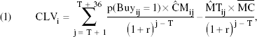
{CLV}_{i} = \sum_{j = T + 1}^{T + 36} \frac{p ({Buy}_{ij} = 1) \times \hat{C} M_{ij}}{{(1 + r)}^{j - T}} - \frac{\hat{M} T_{ij} \times \bar{MC}}{{(1 + r)}^{j - T}},

(1)

where

CLV_i

= lifetime value for customer i,

p(Buy_jj = 1)

= predicted probability that customer i will purchase in period j,

ĈM_ij

= predicted contribution margin provided by customer i in period j,

\hat{M} T_{i j}

= predicted level of marketing contacts (or touches) directed toward customer i in period j,

\bar{M C}

= average cost for a single marketing contact,

= index for future periods (months in this case),

= the end of the calibration or observation time frame, and

= monthly discount factor (.0125 in this case, equivalent to 15% annual rate).

Such a formulation assumes the “always-a-share” approach. In other words, every customer is assumed to be always associated with the firm. Any time interval when the customer does not transact with the firm is assumed to be a period of temporary dormancy. Such an approach is appropriate for noncontractual settings (Rust, Lemon, and Zeithaml 2004; Venkatesan and Kumar 2004), as is the case with the two firms used in this study. For contractual settings, firms can employ the “lost-for-good” approach to compute the CLV (e.g., Berger and Nasr 1998; Lewis 2005). Equation 1 contains the following three terms that must be predicted for each customer:

•

The expected level of marketing contacts, or $\hat{M} T_{ij}$ ;

•

The probability of purchase, or p(Buy_ij = 1); and

•

The contribution margin, or ĈM_ij.

We model the log of the level of marketing contacts for a customer i in time j as follows:

l o g (1 + \hat{M} T_{ij}) = α_{1i} + x_{1ij}^{T} β_{1i} + u_{1ij},

(2)

where x_1ij, β_1i, α_1i, and u_1ij are a vector of predictor variables, a vector of corresponding customer-level coefficients, a customer-level intercept, and an error term, respectively. Use of a logarithmic form of marketing contacts helps account for the diminishing returns of marketing efforts (Venkatesan and Kumar 2004).

To model the probability of purchase, we specify the latent utility for a customer i from the firm in period j as a linear function of predictor variables:

{Buy}_{ij}^{*} = α_{2 i} + x_{2 ij}^{T} β_{2 i} + u_{2 ij},

(3)

where x_2ij, β_2i, α_2i, and u_2ij are a vector of predictor variables, a vector of corresponding customer-level coefficients, a customer-level intercept, and an error term, respectively.

We assume that a customer i purchases from the firm only when his or her latent utility for purchasing from the firm, Buy_ij^*, exceeds a certain threshold, which is set to zero in this case. We do not observe the latent utility of the customer but rather a binary outcome variable, Buy_ij, indicating whether the customer purchased or did not purchase in period j. Consequently, we map the latent utility onto the observed binary outcome variable Buy_ij as follows:

\begin{matrix} \begin{array}{l} {Buy}_{ij}^{*} > 0, {if Buy}_{ij} = 1, \\ {Buy}_{ij}^{*} \leq 0, {if Buy}_{ij} = 0. \end{array} \end{matrix}

Finally, we model the contribution margin from a customer i in period j as follows:

C M_{ij}^{*} = α_{3 i} + x_{3 ij}^{T} β_{3 i} + u_{3 ij},

(4)

where x_3ij, β_3i, α_3i, and u_3ij are a vector of predictor variables, a vector of corresponding customer-level coefficients, a customer-level intercept, and an error term, respectively.

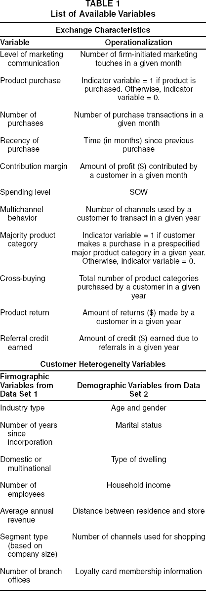
In Equations 2, 3, and 4, the intercept and the other coefficients are specified as customer-specific parameters. In other words, they vary by customer. The variability in parameters is induced by customer heterogeneity, as captured by select firmographic and demographic variables (for the complete list of variables used in this study, see Table 1).

Table 1

List of Available Variables

Exchange Characteristics
Variable	Operationalization
Level of marketing communication	Number of firm-initiated marketing touches in a given month
Product purchase	Indicator variable = 1 if product is purchased. Otherwise, indicator variable = 0.
Number of purchases	Number of purchase transactions in a given month
Recency of purchase	Time (in months) since previous purchase
Contribution margin	Amount of profit ($) contributed by a customer in a given month
Spending level	SOW
Multichannel behavior	Number of channels used by a customer to transact in a given year
Majority product category	Indicator variable = 1 if customer makes a purchase in a prespecified major product category in a given year. Otherwise, indicator variable = 0.
Cross-buying	Total number of product categories purchased by a customer in a given year
Product return	Amount of returns ($) made by a customer in a given year
Referral credit earned	Amount of credit ($) earned due to referrals in a given year

Customer Heterogeneity Variables
Firmographic Variables from Data Set 1	Demographic Variables from Data Set 2
Industry type	Age and gender
Number of years since incorporation	Marital status
Domestic or multinational	Type of dwelling
Number of employees	Household income
Average annual revenue	Distance between residence and store
Segment type (based on company size)	Number of channels used for shopping
Number of branch offices	Loyalty card membership information

Accounting for Missing Transactions

For a given firm (Firm A), the contribution margin from a customer is realized only when Firm A's database records a purchase incidence (i.e., Buy_ij = 1). However, there may be instances when the customer does not make any purchase with Firm A. This could be either because the customer does not have any need to make a purchase or because the customer chooses to buy from a competitor firm. In either case, the proprietary database of Firm A will not record CM_ij when Buy_ij = 0. Equation 4a summarizes this:

\begin{array}{l} C M_{ij} = {CM}_{ij}^{*}, {if Buy}_{ij} = 1, \\ C M_{ij} = {unobserved, if Buy}_{ij} = 0. \end{array}

(4a)

The unobserved CM_ij may include missed purchase incidences when the customer chooses to buy from competitor firms. The lack of information of a customer's transactions with competitors can result in an estimation bias (of customer response elasticity) due to missing data. Kumar and colleagues (2008) address this issue by imputing the missing contribution margin (for customers whose purchase incidence does not occur as expected) on the basis of the historic average interpurchase time of the customer. In such a scenario, the missing contribution margin is imputed as random realizations of a normally distributed prior distribution. However, Kumar and colleagues' approach assumes that the customer will have the same spending level with Firm A as the competitor. In reality, the customer's spending level with the competitor will depend on the customer's SOW with Firm A. For example, a 70% SOW for Firm A implies that the customer spends the remaining 30% of the total category spending with the competitor firms. Consequently, in this study, we assume that the mean of the prior distribution is the product of the customer's average overall contribution margin and the share of the competitor's purchase (as inferred from the observed average contribution margin with Firm A and the SOW data). Kumar and colleagues and Cowes, Carlin, and Connett (1996) discuss the details of the data augmentation process for imputing missing values, and thus we do not repeat it here. However, note that the data augmentation process is used only for obtaining nonbiased estimates of response elasticities. It is not used for the CLV prediction.

The three terms of Equations 2, 3, and 4 are related to the same customer and, as such, are inherently correlated. Thus, we model these three terms jointly as a system of equations. The corresponding likelihood function is as follows:

\begin{matrix} L (MT, Buy, CM) \propto \prod_{i = 1}^{N} \prod_{j = 1}^{T} \Pr {({Buy}_{ij}^{*} \leq 0, {MT}_{ij})}^{1 - {Buy}_{ij}} \\ \times \Pr {(C M_{ij}^{*} = C M_{i j}, {Buy}_{ij}^{*} > 0, {MT}_{ij})}^{{Buy}_{ij}}, \end{matrix}

(5)

where Buy_ij* = customer i's latent utility for purchasing in period j. We estimate the likelihood function using the Bayesian estimation procedure. Technical details of the estimation procedure are in the Appendix.

Segmentation and Profiling

After the CLV scores are computed, managers want to maximize the CE. Computation of the CLV at the individual level offers the flexibility of aggregating customers to virtually any number of discrete segments. In this study, we employ data from two firms—a manufacturing firm catering to business customers and an apparel retail chain catering to retail consumers. The manufacturing firm prefers to create customer segments of size one because each customer represents a business establishment with a relatively high volume of business. Consequently, the manufacturing firm prefers to customize its marketing touches and customer relationship efforts for each of its customers. In contrast, the retail firm has millions of customers with a relatively low volume of business per customer. Consequently, the retail firm prefers to manage its customer base as discrete segments. In either case, for the purpose of this study, we represent the database of both firms as comprising three discrete segments—high CLV, medium/low CLV, and negative CLV—to convey the heterogeneity of customer profitability. After the segments are defined, it is managerially useful to profile the segments to evaluate which demographic (or firmographic) variables vary significantly across segments. We can empirically determine the probability of a customer i belonging to segment q by employing a multinomial logit:

{prob}_{iq} = \frac{\exp (δ_{iq})}{\sum_{q = 1}^{Q} \exp (δ_{iq})}, where δ_{iq} = β_{0} + \sum_{k = 1}^{K} β_{k} X_{iqk},

(6)

where

prob_iq

= the probability of a customer i being in segment q,

δ_iq

= the latent utility of a customer i belonging to segment q,

X_iqk

= the K demographic/firmographic variables corresponding to customer i of segment q, and

β₀, β_k

= coefficients estimated from the data.

Computing CE at the Firm Level

After estimating the CLV for each customer i of the firm, we calculate the CE of N existing or retained customers (CE_R) as the summation of each customer's lifetime value:

{CE}_{R} = \sum_{i = 1}^{N} {CLV}_{i} \cdot

(7)

Another important source of customer value is the new customers the firm expects to acquire in the future. One way to account for this is by predicting the growth of the customer base by applying a diffusion-based model (e.g., Gupta, Lehmann, and Stuart 2004; Kim, Mahajan, and Srivastava 1995). Such an approach can account for nonlinear growth rates and diminishing returns, which is observed as a result of market saturation over time. In the context of our study, we are dealing with two large corporations and predicting the future value of their customers over a relatively short time horizon of three years (as opposed to the infinite time horizon of Gupta, Lehmann, and Stuart's [2004] study). Furthermore, both firms are highly diversified in their respective businesses and are growing over time. Consequently, we apply the average annual growth rate of 6% and 3% for the B2B firm and the B2C firm, respectively. These growth rates of new customers were deemed to be appropriate by both firms for the next three years on the basis of their future business growth plans in terms of acquisitions (for the B2B firm) and opening of new stores (for the B2C firm). Consequently, if M customers are expected to be acquired over the next three years (i.e., 36 months), CE_A represents the CE from M newly acquired customers:

{CE}_{A} = \sum_{k = 1}^{M} \sum_{j = T + 1}^{T + 36} \frac{{CLV}_{kj} - A_{kj}}{{(1 + r)}^{j - T}},

(8)

where

CLV_kj

= the lifetime value for customer k expected to be acquired at time j,

A_kj

= the acquisition cost corresponding to customer k expected to be acquired at time j,

= index for future periods (months in this case),

= the end of the observation time frame, and

= monthly discount factor (.0125 in this case, equivalent to 15% annual rate).

We assume that CLV_kj is equal to the average CLV of the existing customers of the firm (as of time T). Consequently, we need to subtract the acquisition cost A_kj from CLV_kj in Equation 8. For the purpose of computation, we assume that A_kj is equal to the average acquisition cost per customer. These assumptions may not be an accurate representation of CLV_kj for each customer k. However, because this information is eventually aggregated (in the form of CE_A), average CLV measures suffice as a convenient way to compute the CE of new customers for the purpose of this study. Alternatively, some sophistication can be introduced in this computation depending on the firm's sales cycle, nature of business, industry, and availability of data pertaining to customers in the prospect pool. For example, B2B firms typically have long sales cycles, and many B2B firms maintain a sales pipeline report that contains details about each prospective customer. In such a scenario, probability of acquisition can be assigned to each customer and multiplied by the expected CLV. The expected CLV can be determined by matching the profile of the prospective customer with the average CLV of all retained customers of the firm with a similar profile.

The overall CE of all customers of the firm will be the summation of the CE of N retained customers (CE_R) and M newly acquired customers (CE_A), as we depict in Equation 9:

CE = {CE}_{R} + {CE}_{A} \cdot

(9)

Computing MC

Consistent with the efficient market theory and prior research, we compute MC as the market value of the firm. For publicly listed firms, the MC of a firm at time t can be computed as the product of the average stock price (ASP) of the firm and the average number of outstanding shares P of the firm at time t:

{MC}_{t} = {ASP}_{t} \times P_{t \cdot}

(10)

Linking CE to MC

The MC of the firm is linked to the CE of the firm at time t by the following equation:¹

We also tried the logarithmic and quadratic form of CLV_T. However, the linear form of CLV_T as specified in Equation 11 provided the best fit.

{MC}_{t} = γ_{0} + γ_{1} \times {CE}_{t} + ε,

(11)

where γ₀ and γ₁ are parameters to be estimated and ∊_t is the residual term that is assumed to be normally distributed. In this study, time t represents a month.

The term ∊_t represents the difference between the actual and predicted MC in month t, and it represents aspects of firm valuation that are not accounted for by CE_t. The estimate of MC based on CE can be poor if ∊ is large. To address this issue, we let ∊ be a function of factors that are not accounted for in the CLV (and, thus, the CE) computation. As we discussed previously, some inherent risks associated with cash flows are reflected in the MC of the firm (assuming efficient market theory) but not in the CE computation. Consequently, we use the variance in the CE calculation (VAR_CE) and SOW information to capture the volatility and vulnerability in cash flow from customers.

The variance in CE represents the uncertainty in estimating the total lifetime value of customers on the basis of the parameter estimates of the drivers (or covariates) of CLV. This uncertainty arises because of the variance associated with the parameter estimates (of Equations 2, 3, and 4) that are used to compute CLV. Thus, we estimate the lifetime value of each customer by making a draw of customer-level parameter estimates. We then add up the CLV of each customer to get the total CLV (i.e., CE). If we repeat this process 10,000 times, each process/iteration will generate a different value of CE. Consequently, a distribution of CE is generated, thus facilitating the calculation of VAR_CE. On the basis of such an operationalization, we expect VAR_CE to have a negative impact on the MC of the firm.

Another dimension of risk is in the form of vulnerability of cash flows. We capture this through the SOW information. We operationalize the average SOW across customers as a weighted average (weighted by the contribution margin of the customers) to give more importance to high-value customers and less importance to low-value customers. We expect SOW to exert a positive influence on MC, as discussed previously. In other words, a high SOW implies greater stability of cash flow from customers, thus lowering the risk of the firm's operations and raising the MC of the firm.

Inclusion of these risk factors can help explain why two firms that have similar CE values can still have dissimilar market valuation because of the differences in perceived risk of the two firms. Consequently, these risks moderate the relationship between the CE and the MC of the firm and thus exert their influence as both main effects and interaction terms as specified in Equation 12.

In addition to cash flow risks, there may still be some unobserved effects related to the environment and the market (e.g., investor sentiments, macroeconomic factors) that could bias the parameter estimates. To mitigate this issue, we employ one-period lagged values of MC as a proxy for omitted variables. Therefore, we can express ∊ in time t as follows:

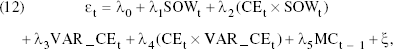
\begin{matrix} ε_{t} = λ_{0} + λ_{1} {SOW}_{t} {+ λ}_{2} ({CE}_{t} \times {SOW}_{t}) \\ + λ_{3} {VAR_CE}_{t} + λ_{4} ({CE}_{t} \times {VAR_CE}_{t}) + λ_{5} {MC}_{t - 1} + ξ , \end{matrix}

(12)

where λ is a vector of parameters to be estimated representing the effect of risk factors and unobserved factors that are accounted for in the MC value but not in the CE computation. Note that the impact of these factors on the MC of the firm is constrained by the magnitude of the residual term e_t This ensures that the relationship between the CE and the MC is maximized and not confounded by potential collinearity with terms specified in Equation 12.²

We test for issues related to autocorrelation of error terms using standard diagnostic tests and find that this does not significantly affect our results. The CE term is statistically significant even if all terms in Equations 11 and 12 were to be estimated as a single equation.

The CE_t term in Equations 11 and 12 represents the total lifetime value of customers by keeping a finite future time horizon of three years. It could be argued that some alternative future time horizon for CE computation (i.e., less than or more than three years) may provide a stronger relationship between the CE and the MC of the firm. Thus, we tested the linkage between CE and MC by plugging in the CE estimates (as per Equations 1, 2, 3, and 4) for different future time horizons.

Data Description

We employ customer transaction data sets of firms from two industries representing the B2B and the B2C settings. Both firms are large, publicly traded companies.

The B2B data set comes from a Fortune 1000 high-tech manufacturing firm that sells computer-related hardware and supporting software. The company's database focuses on business customers and contains monthly transaction data for all its customers (establishments) from January 2000 to April 2007. The product categories in the database represent different spectrums among high-technology products. For these product categories, it is the choice of the buyer and the seller to develop their relationships, and there are significant benefits to maintaining a long-standing relationship for both. Although these products are durable goods, they require constant maintenance and frequent upgrades; this provides the variance required in modeling the customer response. To help the manager make a decision, he or she has access to each customer's date of each purchase, the product category purchased (and, thus, the level of cross-buying within the firm), the channel used by the customer to transact business (e.g., online versus direct sales), and the amount spent at each purchase occasion. The SOW information is obtained from a third-party external research firm hired by the B2B high-tech firm. In addition, the high-tech firm has developed a sophisticated approach to impute the SOW for each of its customers. We use both sources of information to reconcile the differences in SOW, if any.

The B2C data set comes from a large retail chain that sells ready-to-wear clothes, shoes, and accessories for both men and women. The retailer's data set contains customer-level, monthly transaction data for all its more than one million customers who made purchases between January 2000 and April 2007. The retailer offers its customers three ways to make their purchases: (1) through any of the company's 30 retail stores in the United States, (2) through a shopping catalog, and (3) through the company's Web site. Thus, the data set captures information on multichannel shopping behavior. The data set also contains rich information on different product categories the retailer is selling. Purchase transaction details, such as frequency of purchase, average purchase value, type of product purchased, number of product categories purchased, the channel through which the purchase was made, and the number and type of marketing communications made to the customer by the firm, are available for each month. The retailer calculates the SOW information as the ratio of the total amount of dollars spent by a given customer in one year (with the retailer) to the estimated total amount of dollars the customer is capable of spending on similar products in one year. The denominator is imputed on the basis of available demographic information of the customer, such as zip code, gender, marital status, family size, income, and age.

For both data sets, we divide the customers into two samples. Sample 1, the “model-building sample,” comprises 70% of the total customers of the firm. Sample 2, the “model-validation sample,” comprises 30% of the customers of the firm. We use Sample 1 to calibrate the model and Sample 2 to validate the calibrated model. We then use the final model to compute the CLV for the entire sample set. Figure 3 depicts the data set in terms of associated timelines used for data analyses and prediction.

Figure 3

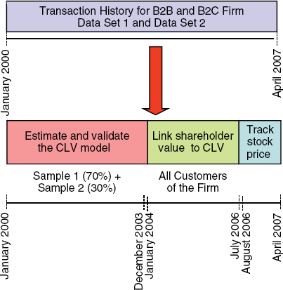
Data Analyses: Timelines

The unique strength of the two data sets lies in the availability of longitudinal transaction data for each customer of the firm. This enables us to compute CLV at the individual customer level, uncover customer-centric measures that drive CLV, and subsequently test the impact of customer-centric tactics/strategies on the MC of the firm. Most important, disaggregated data facilitate deployment of marketing strategies at customer segments even as small as size one.

Table 1 summarizes the set of customer-level variables that are employed from the two data sets to estimate the propensity to buy, the contribution margin and marketing contacts for each customer, and, thus, the lifetime value of each customer. We draw the choice of variables from prior research as well as theoretical and practical considerations that typically govern CLV prediction (for a discussion, see Kumar, Shah, and Venkatesan 2006; Venkatesan, Kumar, and Bohling 2007). The availability of firmographic (for the B2B customers) or demographic (for the B2C customers) variables corresponding to customers in data set 1 and data set 2, respectively, help in estimating customer-specific parameters of Equations 2, 3, and 4, as well as in conducting profile analyses as specified in Equation 6. For the B2B firm, we use average firm revenue, firm size (determined by the number of employees), and industry type to estimate the customer-specific coefficients. For the B2C firm, we use gender, household income, and distance from the store (as determined from zip code) to estimate customer-specific coefficients.

Estimation

The objective of our estimation is to recover two sets of parameters: Θ₁ and Θ₂. Let Θ₁ represent the set of parameters pertaining to CLV computation (i.e., customer-level parameters corresponding to Equations 2, 3, and 4), and let Θ₂ represent the set of parameters pertaining to linking CE to MC (i.e., firm-level parameters corresponding to Equations 11 and 12). The estimation procedure is carried out in a sequential manner.

We begin by dividing the firms' customers corresponding to the period January 2000 to December 2003 into two samples (see Figure 3). Sample 1 corresponds to 70% of the customers, and Sample 2 corresponds to 30% of the customers (randomly drawn from the firms' databases). We use Sample 1 to estimate Θ₁. Then, we apply the set of parameters represented by Θ₁ to estimate the CLV of customers in Sample 2. In other words, we use Sample 1 to calibrate the model and Sample 2 to validate the model. The validation sample results in a mean absolute percentage error of 17%, which is deemed to be reasonable.

To estimate Θ₂, we use Θ₁ to compute the CLV for all customers (i.e., CE) as of month t (e.g., January 2004) and then measure the MC (based on the observed stock price) as of the end of month t (i.e., January 31, 2004). We repeat this process for every month, while moving forward one month at a time for the period spanning January 2004 to July 2006. Consequently, by July 31, 2006, we obtain 31 values of CE (as predicted by the parameters in Θ₁) and 31 values of MC (as computed from the observed value of average stock price). We then use these 31 data points to regress MC on CE and variables representing cash flow risk and unobserved factors. The outcome of regression is parameter estimates for Θ₂.

For Part 2 of this study, we use Θ₁ and Θ₂ to compute CE and to predict MC, respectively, for each month during a time frame from August 2006 to April 2007. Figure 3 provides a brief overview of various timelines used for model estimation, validation, prediction, and tracking.

Results and Discussions for Part 1

For the B2C firm, we report the coefficient estimates of the drivers of CLV in Table 2. The reported values are the posterior means and variances. In the interest of space, we present the parameter estimates only for the B2C firm. For the B2B firm, the results obtained are similar to all coefficient estimates for the B2C firm, having identical signs but differing magnitudes. A parameter is considered “not significant” if a zero exists within the 2.5th percentile and the 97.5th percentile values of the posterior distribution for that parameter. Note that the inclusion of lagged values of covariates facilitates prediction and interpretation of causality. Furthermore, we include a relationship duration indicator as a binary variable in all three models. The value of this binary variable is 1 for a customer who originated with the firm before January 2000 (i.e., before the observation window used for analysis) and 0 for a customer who originated with the firm on or after January 2000 (i.e., within the observation window used for analysis). The results for all parameter estimates appear in Table 2. The direction of the sign for all variables is consistent with previous research studies on CLV computation at the individual customer level (e.g., Kumar, Shah, and Venkatesan 2006; Venkatesan and Kumar 2004).

Table 2

Parameter Estimates for the CLV Model (B2C Firm)

Independent Variables	Coefficients^a
Independent Variables	M	Variance
Level of Marketing Contacts
Relationship duration indicator	3.868	.0471
Lagged level of market communication	.682	.0212
Lagged average number of purchases	.393	.0176
Lagged spending level	.427	.0274
Loyalty program member	2.187	.0262
Lagged level of cross-buying	.312	.0481
Recency of purchase	−.162	.0168
Square of recency of purchase	.009	.0014
Lagged average contribution margin	.582	.0467
Purchase Incidence
Relationship duration indicator	.412	.0386
Lagged indicator of purchase	.676	.0526
Lagged spending level	.008	.0012
Lagged average contribution margin	.101	.0267
Log of lagged level of contacts	.007	.0014
Lagged level of cross-buying	.281	.0646
Recency of purchase	−.052	.0087
Lag of multichannel behavior	.386	.0375
Contribution Margin
Relationship duration indicator	.091	.0122
Lagged contribution margin	.729	.0395
Lagged average contribution margin	.686	.0267
Lagged level of cross-buying	.391	.0291
Loyalty program member	.137	.0156
Log of lagged level of marketing
communication	.146	.0217
Lag of multichannel behavior	.426	.0428
Lag of product returns	.153	.0354
Lag of square of product returns	−.0621	.0196

We computed mean and variance using the 5th through 95th percentiles of the posterior sample.

The results for the marketing contacts model show that the firm tends to contact a customer more frequently if that customer has historically been contacted frequently, made more purchases, spent more dollars with the firm, been a member of the loyalty program, and/or purchased a greater number of products. The recency of purchase shows an inverted U-shaped relationship to marketing contacts, indicating that the firm tends to contact a customer who has not made a purchase in the recent past. However, the firm's tendency to contact a person diminishes if the customer fails to make any purchase beyond a certain threshold.

The results for the purchase incidence model indicate that a customer is more likely to purchase if he or she has historically made a purchase, spent more dollars with the firm, been contacted by the firm through marketing initiatives, purchased a greater number of products, transacted through multiple channels, and/or not made any purchases in the recent past.

The results for the contribution margin model indicate that the expected contribution margin of the customer is high if the customer has historically spent more, purchased a greater number of products, been enrolled in a loyalty program, been contacted by the firm through direct marketing, and/or shopped through multiple channels of the firm. The contribution margin has an inverted U-shaped relationship to product returns, which is consistent with prior findings.

We use the coefficient estimates to calculate the CLV score for each customer as expressed in Equation 1. To get an idea of the distribution of CLV scores, we first rank all customers in descending order. Then, we aggregate customers into deciles so that each decile represents 10% of the customer base and the CLV corresponding to each decile is the average CLV of customers within the decile. Such a transformation aids in displaying the distribution of CLV scores across customers in a diagrammatic form (as Figure 4 shows). The distribution of CLV for both firms is heavily skewed. For the B2B firm (see Figure 4, Panel A), the top 20% of the customers account for 91% of total profits, while the bottom 20% have negative lifetime values. For the B2C firm (see Figure 4, Panel B), the top 20% of the customers account for 93% of the firm's profits, while the bottom 30% are a drain on the company's resources with negative lifetime values. For ease of explanation and further analysis, we divide the customer base of both firms into three discrete segments: high CLV (the top 20% of customers for both firms), medium/low CLV (the middle 60% and the middle 50% of customers for the B2B and B2C firms, respectively), and negative CLV (the bottom 20% and the bottom 30% of customers for the B2B and B2C firms, respectively).

Figure 4

Distribution of CLV Scores

Do customers who differ in CLV have any distinguishing demographic or firmographic characteristics? The answer lies in the results of the profile analyses. Table 3 captures the distinguishing characteristics of a typical high-CLV and a typical negative-CLV customer for the B2B firm and the B2C firm, respectively. The results indicate that for the B2B firm, a typical high-CLV customer is a well-established multinational organization from a high-technology, aerospace, or financial services industry that employs more than 500 employees, has been in business for 15–25 years, and has annual revenue in excess of $50 million. In contrast, a typical negative-CLV customer for the B2B firm is a domestic organization from the chemicals or plastics industry that employs approximately 100–300 employees, has been in business for 5–10 years, and has average annual revenue in the range of $5–$10 million. For the B2C firm, a typical high-CLV customer is a married woman, is 30–40 years of age, has a household income in excess of $95,000, lives in a house that is relatively close to the store, and is enrolled in the store's loyalty program. A typical negative-CLV customer for the B2C firm is a single man, is 20–30 years of age, earns less than $60,000, lives in a rented apartment that is relatively far from the store, and is not a member of the store's loyalty program.

Table 3

Profile of a Typical High- and Negative-CLV Customer

A: The B2B Firm
Firmographic Variable	Typical High-CLV Customer	Typical Negative-CLV Customer
Industry type	High-tech, aerospace, financial services	Chemicals and plastics
Number of years since incorporation	15–25 years	5–10 years
Domestic or multinational	Multinational	Domestic
Number of employees	>500 employees	100–300 employees
Average annual revenue	>$50 million	$5–$10 million

B: The B2C Firm
Demographic Variable	Typical High-CLV Customer	Typical Negative-CLV Customer
Age	30–40 years	20–30 years
Gender	Female	Male
Marital status	Married	Unmarried
Type of dwelling	Own	Rent
Household income	More than $95,000	Less than $60,000
Distance between residence and store	Less than 10 miles	More than 10 miles
Number of channels used for shopping	2 or 3	1 or 2
Loyalty card membership	Enrolled	Not enrolled

Note that the results from the profile analyses do not necessarily indicate that all customers having the profile of a high-CLV customer will have a high CLV, and vice versa for negative-CLV customers. The profile analyses results merely indicate that, on average, there is a relatively high probability of finding high- and negative-CLV customers with the profile description in Table 3.

After conducting profile analyses, we test the relationship of CE to MC for different time horizons of CLV computation. Essentially, we compute CLV with one-, two-, and three-year time horizons and evaluate the fit between the CE and the MC of the firm. The results in Table 4 indicate that the CLV prediction with a three-year horizon results in the best fit between CE and MC for both the B2B and the B2C firms.³ In addition, Table 4 shows the extent of improvement in the relationship between CE and MC when we include measures of risk (i.e., SOW and VAR_CE) in the analysis. The R-square for the model improves by 15% for the B2B firm and by 8% for the B2C firm when we add the measures of risk. There is a further improvement (R² = 77% for the B2B firm and 79% for the B2C firm) when we include the lag of MC in the model to account for the impact of the omitted variables. The improvement in R-square is statistically significant for all cases (after we account for changes in the degrees of freedom).

The prediction of CLV beyond three years deteriorated the relationship between CE and MC. This could be due to loss of prediction efficiency (at the individual customer level) beyond a time horizon of three years.

Table 4

Comparison of Model Performance

Measurement Condition for CE–MC Equation	Model Performance (R²)
Measurement Condition for CE–MC Equation	B2B Firm	B2C Firm
CLV computed with a one-year time horizon	.26	.28
CLV computed with a two-year time horizon	.30	.34
CLV computed with a three-year time horizon	.33	.38
Measurement Condition for CE–MC Equation with CLV Computed Over a Three-Year Time Horizon
After adding measures of volatility and vulnerability	.48	.46
After adding past shareholder value	.77	.79

Next, we evaluate whether measures of volatility, vulnerability, and past MC values are significant predictors of MC (as specified in Equation 12). The results appear in Table 5. As we expected (and discussed previously), SOW and past MC have a positive impact on MC, while VAR_CE has a negative relationship to MC. All hypothesized relationships are statistically significant.

Table 5

Results for Linking CE and MC

Variable	Parameter Estimate (SE)
Variable	B2B Firm	B2C Firm
Intercept	16.21 (2.96)	9.62 (1.81)
CE	3.47 (.68)	1.86 (.42)
SOW	1.55 (.27)	.90 (.18)
VAR_CE	−5.96 (1.33)	−3.04 (.76)
CE × SOW	.836 (.317)	.561 (.186)
CE × VAR_CE	−1.142 (.393)	−1.06 (.329)
Lag of MC	.49 (.06)	.45 (.07)

In summary, we obtain the best linkage between CE and MC when we predict the CLV for a three-year time horizon, include measures of volatility and vulnerability, and account for the effect of unobserved factors. Thus far, the results help establish that the MC of the firm is closely tied to the CE of the firm. Armed with these results, can the firm deploy marketing initiatives to increase the stock price of the firm?

Previously, we observed a heavily skewed distribution of customer profitability (see Figure 4). This implies that different customers have different impacts on the firms' bottom line. To quantify the differential impact, we perform a simulation exercise to compute the change in CE after increasing the acquisition rate of the firms' customers by 1% and increasing the cross-buy (applicable for the firms' retained customers) by one product. Next, we apply the CE–MC relationship to calculate the corresponding change in MC. Our results indicate that a 1% increase in the acquisition rate of customers could translate into a 1.4% and 1.9% increase in MC for the B2B and the B2C firm, respectively. Similarly, an increase in cross-buying by one product across all retained customers could translate into a 5.3% and a 7.5% increase in the MC for the B2B and the B2C firm, respectively (see Table 6, Panel A). We repeat the simulation by applying the 1% increase in acquisition rate and the increase in cross-buying (by one product) for the high-CLV, medium-/low-CLV, and negative-CLV customers separately. The results indicate that the lift in MC (in percentage terms) is three times as much when acquisition and cross-selling efforts are targeted only to high-CLV customers rather than to all customers of the firm. Furthermore, the MC of the firm drops if the firm acquires the wrong customers (i.e., customers who subsequently end up with negative CLV), while the MC of the firm increases only marginally when negative-CLV customers buy an additional product (see Table 6, Panel A).

Table 6

Measuring the Impact on MC

A: Expected Impact on MC due to Increase in Acquisition Rate and Cross-Sell
Increasing Acquisition Rate by 1%	Impact on MC
Increasing Acquisition Rate by 1%	B2B Firm	B2C Firm
For all customers	↑ 1.4%	↑ 1.9%
For high-CLV customers	uarr; 7.9%	uarr; 9.2%
For medium-/low-CLV customers	uarr; 0.8%	uarr; 2.0%
For negative-CLV customers	↓ 3.0%	↓ 3.1%
Increasing Cross-Buy by One Product
For all customers	↑ 07.2%	↑ 08.3%
For high-CLV customers	↑ 18.1%	↑ 21.6%
For medium-/low-CLV customers	↑ 05.1%	↑ 06.8%
For negative-CLV customers	↑ 02.1%	↑ 01.8%

B: Actual Impact on MC due to Implementation of CRM Strategies
Customer Segment	Effect of CRM Strategies (Lift in CE)
Customer Segment	B2B Firm	B2C Firm
All Segments	19.4%	23.3%
High CLV	44%	41%
Medium/low CLV	20%	18%
Negative CLV	8%	7%

The results in Table 6, Panel A, underscore the importance of customer heterogeneity in driving firm value. Therefore, it would be more impactful for the firm to improve acquisition and cross-selling for only the high-CLV customers rather than extending those improvements across all customers of the firm. Marketing resources are potentially wasted when directed toward the wrong customers (e.g., customers with a negative CLV).

In Part 2 of our study, we advance the results of Part 1 to demonstrate how the two real-world firms deploy CLV-based differentiated customer management tactics and strategies. We track the outcome in terms of the actual stock price movement of the firms.

Part 2: Lifting the Stock Price of the Firm

Methodology and Results

In our previous discussions, we showed the conceptual link between our key input, marketing interventions, and our key outcome, the stock price of the firm (see Figure 2). To put that concept into practice, any marketing manager who wants to implement the proposed framework would need to deploy marketing initiatives that are directed at increasing the CE of the firm. We collectively refer to these marketing initiatives as CRM strategies. We presented different CRM strategy options (see Kumar 2008) to the B2B and B2C firms used in this study and asked for their cooperation in implementing one or more of these strategies to allow us to track the outcome in terms of the stock value of the firm.

Strategy implementation

The B2B firm implemented the following CRM strategies: (1) resource reallocation, (2) selective acquisition, and (3) multichannel behavior. The B2C firm implemented the following strategies: (1) customer selection (2) cross-selling, and (3) multichannel behavior.

The B2B firm implemented the resource reallocation strategy by reallocating a portion of marketing resources from the medium-/low-CLV and the negative-CLV customers to the high-CLV customers. It implemented the selective acquisition strategy by focusing customer acquisition resources on prospective customers that matched the profile of the high-CLV customers. The multichannel behavior strategy that both firms implemented entailed offering special incentives to the high-CLV and the medium-/low-CLV customers to shop from more than one channel while directing negative-CLV customers to transact (including customer service) only through the online channel. The B2C firm implemented the customer selection strategy by selecting customers on the basis of their CLV score for proactive relationship-building initiatives, such as special rewards and shopping privileges. The B2C firm implemented the cross-selling strategy by sending promotion incentives (through direct marketing) to relevant customers to induce cross-buying. The firm used proprietary cross-selling models to determine which product to offer to which customer. The nature of the promotion incentives offered varied by the type and lifetime value of each customer. For example, high-CLV customers were offered unconditional incentives to purchase a new product category, while some medium-/low-CLV customers and all negative-CLV customers were offered cross-buying incentives contingent on minimum spending ($30 on average). Implementation of these CRM strategies had a direct influence on the principal drivers of CLV—namely, contribution margin, number of purchases, recency of purchase, cross-buying, and so on—thus increasing the overall CE of the firm. As Table 6, Panel B, shows, the various CRM strategies showed an average CE lift of 19.4% for the B2B firm and 23.3% for the B2C firm during the observation period.

Table 6, Panel B, also summarizes the lift in CE (due to CRM strategies) by high-CLV, medium-/low-CLV, and negative-CLV customers. As we expected, high-CLV customers showed the highest lift in CE after the application of relevant CRM strategies.

Evaluating the impact on stock price

The marketing/sales teams of the two firms were successful in implementing CRM strategies that resulted in an increase in the CE of the firm (see Table 6, Panel B). However, did this translate into any positive impact on the stock value of the firm? To find out, we compared the stock price movement of the two firms nine months before and after implementation of CLV-based CRM strategies (i.e., nine months around July 2006) (see Figure 5).⁴ We find that the percentage increases in stock price (relative to the July 2006 stock prices) for the B2B firm and the B2C firm are approximately 32.8% and 57.6%, respectively, at the end of the observation window (i.e., nine months after the CLV-based strategy implementations). However, to what extent can we predict such increases in stock price on the basis of changes in CE?

Note that the strategies were actually rolled out by the two firms over a period of three months spanning from June to August 2006. Consequently, we would expect to begin to observe the full benefits of the strategies after August 2006.

Figure 5

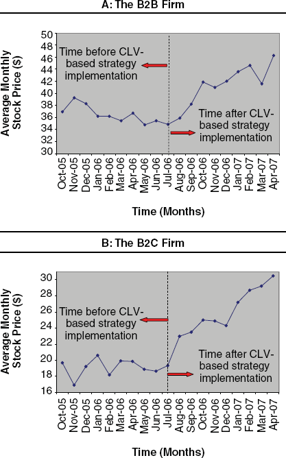
Actual Stock Price Movement

We apply the CE–MC relationship developed in Part 1 to predict the MC of the firm for each future month t and repeat this procedure throughout the observation period of August 2006–April 2007 (i.e., we update the value of the CE and MC prediction for each month as new information becomes available). By doing so, we compute nine monthly values of MC based on CE predictions. We then divide the MC by the number of outstanding shares of the firm to arrive at nine monthly average values of the stock price of the firm. We plot these values over time and compare them with the actual average values of the stock prices of the two firms (see Figure 6). The results indicate that we can track the actual movement of stock prices within a maximum deviation range of 12% to 13%.

Figure 6

Actual Versus Predicted Stock Price

Thus, implementation of CLV-based marketing strategies increases the stock price of the firm, and the increase can be reasonably predicted with customer-level drivers of the CE of the firm. In such a scenario, the CEO would be interested in whether such an increase in stock price can beat market expectations. In other words, can the increases in the stock prices of the two firms be attributed to shareholder value creation? To answer this question, we compare the stock price movements of the two firms with Standard & Poor's (S&P) 500 index during the August 2006–April 2007 observation period (see Figure 7). The S&P 500 is a commonly used index by financial analysts to benchmark the stock performance of a firm (especially for large firms). To adjust for differences in scale, we normalize the stock price and the index value movements to percentage changes with respect to a reference value. We used the average values of the stock prices of the two firms and the S&P 500 index as of July 2006 (i.e., the time immediately preceding CRM strategy implementation) as reference values. Figure 7 indicates that the stock prices of both firms consistently outperform the S&P 500 during the observation window. The B2B firm outperforms the S&P 500 by 2 times as much, and the B2C firm outperforms the S&P 500 by 3.6 times as much.

Figure 7

Comparison of Stock Price Movement with the S&P 500 Index

If we assume the performance of the S&P 500 index as the baseline expected performance of the two firms, the area between the curves (denoted by A and B in Figure 7, Panels A and B, respectively) can be attributed to shareholder value creation due to the CLV-based marketing strategies implemented by the marketing/sales teams of the two firms. Note that the area between the two curves progressively increases over time. This is because the tactics and strategies the two firms deployed are expected to have some lead time before showing concrete results in the form of a dollar increase in revenue and stock price. Furthermore, the purchase cycle of the B2B firm's customers is longer than the purchase cycle of the B2C firm's customers. Consequently, the B2C firm shows a faster rise in stock price than the B2B firm during the observation window after the deployment of CRM strategies.

We also benchmark the stock performance of the two firms by comparing it with the average stock performance of three of their closest competitors (as identified by the two firms and leading stock analysis portals). We find that the B2B firm's stock increases by 32.8% during the observation period, while its competitors' stock goes up by an average of 12.1% over the same period. Similarly, the B2C firm's stock increases by 57.6%, while its competitors' stock goes up by an average of 15.3% over the same period.

Managerial Implications

Expanding the Role of Marketing and the Marketer

One of the greatest challenges that marketers face today is the marginalization of their relative importance to the firm (Nath and Mahajan 2008). Possible reasons lie in the failure of the marketer to accurately prove his or her worth and/or the inability to relate marketing performance to reliable financial metrics (Lehmann 2004; Rust, Lemon, and Zeithaml 2004). The proposed framework in this study enables marketing managers to deploy marketing initiatives at the customer level and to quantify the outcome through a high-level financial metric, such as the stock price of the firm. By doing so, marketers can demonstrate the impact of the marketing organization on driving the boardroom's primary agenda of increasing the overall value of the firm. Consequently, implementation of the proposed framework bears the promise of augmenting both the scope and the importance of the marketer and the marketing function in virtually any organization. A direct benefit of this could result in the marketing function being allocated a greater portion of the firm's resources relative to other competing functions, such as information technology, manufacturing, and research and development.

Aligning the CMO's Objectives with the CFO's Agenda

Our study proposes a methodology to illustrate how marketing strategies and tactics can be linked to financial measures, and by doing so, we hope to bridge the gap between the CMO's objectives and the CFO's agenda. This is important because more often than not, the performance metrics used by marketing (e.g., advertisement recall, brand awareness, customer satisfaction scores, net promoter score) are not well appreciated by the CFO, who typically wants the performance impact to translate into the financial language that he or she understands. The performance metric of MC is well understood not only by the CFO but also by the CEO and other important stakeholders of the firm, such as the shareholders.

Managing Customers' Profits and Cash Flow Risks

Prior research has clearly shown the benefits of customer centricity (e.g., Shah et al. 2006) and how CLV- or CE-based strategies can lead to increased profitability for a firm (e.g., Kumar et al. 2008; Rust, Lemon, and Zeithaml 2004). This study goes a step further to demonstrate empirically which customer-specific measures are responsible for driving future profits, for which customers, and to what extent. Furthermore, our framework recognizes that the future profit stream is susceptible to certain risks, which can be quantified through customer-centric measures, such as SOW and variance in CLV computation. Consequently, our framework can help marketers manage profit and risk simultaneously through specific marketing interventions directed at specific customers.

Future Directions

This study addresses the substantive topic of how marketers can increase the MC of the firm. Although this has substantive managerial implications, we hope to motivate researchers to contribute further to this exciting stream of research. The following is a discussion of some important issues that could be addressed by future studies.

Sustainability of Stock Price Gains

Our study shows how the increase in CE can be linked to the increase in stock price and that the relationship exists for at least nine months after the implementation of the relevant CRM strategies. However, it may be worthwhile to empirically test whether this holds true for longer time horizons. Furthermore, it may be worthwhile to determine whether stock price gains are sustained when factoring in competitive actions and reactions. For example, what would have happened if the marketing tactics of the two firms used in the study were imitated by competitors? Would the stock price have risen by the same level? Another possibility is competitors adopting a CLV-based framework and thus replicating the strategic actions of the two firms. Would this marginalize the firm's competitiveness and translate into a subdued gain in market value? These are promising areas for further research.

Applicability of Framework

Our study is suitable for relatively large and mature publicly traded firms whose primary source of revenue is from doing business with their customers. There may be cases in which some firms have other sources of sizable income, such as investments, rental fees, and licensing fees. In such cases, Equation 11 can be modified by including more terms (in addition to the CLV) to acknowledge the additional sources of cash flow that could significantly affect the MC of the firm. Furthermore, this study estimates CLV over a future time horizon of three years. During this period, both firms in the study anticipate continuous growth and nonsaturation of their market. However, this may not hold true for firms from other industries (e.g., telecommunications) that are experiencing market saturation. In addition, our assumptions may not be valid over longer time horizons, in which firms in general may eventually experience a slowdown in business because of the increasing difficulty of acquiring profitable customers, leading to diminishing contribution margins over time. Future studies could address these issues by extending the framework to different industry settings and/or time horizons.

Efficient Market Theory

The proposed framework is based on the assumptions of efficient market theory. Accordingly, we expect the stock market to respond efficiently in response to changes in the CE of the firm. However, this would not hold true if efficient market theory is challenged. For example, research in behavioral finance has shown that investors tend to react more strongly (and often irrationally) to bad news than to good news (Kahneman and Tversky 1979). In addition, stock prices in emerging markets are often influenced by investor sentiments rather than economic fundamentals (Barberis, Shleifer, and Vishny 1998). In such a scenario, the relationship between CE and MC will be weaker than what we found in this study.

Investing in Customers versus Investing in Brands

Our study gives examples of how investment in customer-based initiatives (e.g., cross-selling, optimal resource allocation) can increase the CE and, thus, the MC of the firm. What about investing in brands? Our contention is that firms should continue to invest in brands as long as doing so contributes to increasing CE and lowering cash flow risk. For example, a firm's investment in brand-related initiatives, such as advertisements, can result in increasing the SOW of its customers and/or increasing the purchase probability due to an increase in brand awareness. Rust, Zeithaml, and Lemon (2004) offer a compelling discussion on how investment in brands should be governed by CE. Kumar, Luo, and Rao (2008) present an empirical framework to link brand value to CLV.

Conclusion

The findings from this study empirically demonstrate the power of marketing in shaping firm value. We also hope to equip the marketer with the means to broaden the scope and importance of marketing. Will the CMO (or the senior marketer) rise to the challenge? Will the CMO be able to vindicate his or her role from being redundant (Nath and Mahajan 2008) or most frequently fired (Welch 2004) to that of an invaluable executive within the organization? The answer has far-reaching implications on the future of how marketing will be perceived within firms.

Footnotes

Technical Details

The formulation of Equations 2, 3, and 4 is similar to the seemingly unrelated regression model structure, such that the predictor variables in the equations need not be the same. We assume the covariance structure of the errors in Equations 2, 3, and 4 to be as follows:

Such a covariance structure allows for correlation across the residual terms. We fix σ₁₁ to be equal to 1 to ensure model identification. The covariance structure of the errors accounts for any unobserved dependence among MT_ij, Buy_ij, and CM_ij. By letting β = [β₁,β₂,β₃] and α = [α₁,α₂,α₃], the system-of-equations model gives rise to the likelihood specified in Equation 5.

We obtain the customer-specific intercept terms (for Equations 2, 3, and 4) from a multivariate normal distribution:

where

We obtain the customer-specific coefficients (for Equations 2, 3 and 4) from a multivariate normal distribution:

where

For both the B2B firm and the B2C firm, p = 3. For estimation, we assume diffuse and conjugate priors for the model parameters. We assume multivariate normal priors for Ψ and Δ. Let Ψ denote the dimension of the Ψ vector; then, the prior specification of Ψ is given as Ψ ∼ MVN(_μΨ, Σ_Ψ, where μ_Ψ is a d_Ψ-dimensional column vector of zeros and Σ_Ψ = 100I_dΨ, where I_dΨ> is a (d_Ψ × d_Ψ)-dimensional identity matrix. Similarly, let d_Δ denote the dimension of Δ; then, the prior specification of Δ is given as Δ ∼ MVN (μ_Δ, Σ_Δ), where μ_Δ is a d_Δ-dimensional column vector of zeros and Σ_Δ = I_dΔ, where I_dΔ is a (d_Δ × d_Δ)-dimensional identity matrix.

We assume inverse Wishart priors for the variance parameters. The prior specification for Σ_β is given as Σ_β = IW(ρI_dΨ>, ρ), where ρ = 15 and I_dΨ is a (d_Ψ × d_Ψ)-dimensional identity matrix.

Similarly, the prior specification for Σ_α is given as Σ_α = IW(ρI_dΔ, ρ), where ρ = 15 and I_dΔ is a (d_Δ × d_Δ)-dimensional identity matrix. The prior specification for Σ_y is given as Σ_y = IW(15I₃, NT), where I₃ is a (3 × 3)-dimensional identity matrix. For details on data augmentation, refer to Cowles, Carlin, and Connett (1996).

References

ANA & Booz Allen Hamilton (2004), “Are CMOs Irrelevant? Organization, Value, Accountability, and the New Marketing Agenda,” (accessed November 15, 2007), [available at http://www.boozallen.com].

Anderson

Eugene W.

, Fornell

Claes

, and Mazvancheryl

Sanal K.

(2004), “Customer Satisfaction and Shareholder Value,” Journal of Marketing, 68 (October), 172–85.

Barberis

, Shleifer

, and Vishny

(1998), “A Model of Investor Sentiment,” Journal of Financial Economics, 49 (3), 307–343.

Bauer

Hans H.

, Hammerschmidt

Maik

, and Braehler

Matthias

(2003), “The Customer Lifetime Value Concept and Its Contribution to Corporate Valuation,” Yearbook of Marketing and Consumer Research, 1, 47–66.

Berger

P.D.

, Echambadi

, George

, Lehmann

D.R.

, Rizley

, and Venkatesan

(2006), “From Customer Lifetime Value to Shareholder Value,” Journal of Service Research, 9 (2), 156–67.

Berger

P.D.

, and Nasr

N.I.

(1998), “Customer Lifetime Value: Marketing Models and Applications,” Journal of Interactive Marketing, 12 (1), 17–29.

The CMO Council Report (2007), “Define & Align the CMO: 2007,” (accessed January 15, 2008), [available at http://www.cmocouncil.org].

Cowles

M.K.

, Carlin

B.P.

, and Connett

J.E.

(1996), “Bayesian Tobit Modeling of Longitudinal Ordinal Clinical Trial Compliance Data with Nonignorable Missingsness,” Journal of the American Statistics Association, 91 (433), 86–98.

Doyle

Peter

(2000), Value-Based Marketing. Chichester, UK: John Wiley & Sons.

10.

Fader

Peter

, Hardie

Bruce

, and Lee

Ka Lok

(2005), “RFM and CLV: Using Iso-CLV Curves for Customer Base Analysis,” Journal of Marketing Research, 42 (November), 415–30.

11.

Fama

Eugene F.

(1970), “Efficient Capital Markets: A Review of Theory and Empirical Work,” Journal of Finance, 25 (May), 383–417.

12.

Fornell

Claes

, Mithas

Sunil

, Morgeson

Forrest

, and Krishnan

M.S.

(2006), “Customer Satisfaction and Stock Prices: High Returns, Low Risk,” Journal of Marketing, 70 (January), 3–14.

13.

Gupta

Sunil

, and Lehmann

Donald R.

(2005), Managing Customers as Investments: The Strategic Value of Customers in the Long Run. Upper Saddle River, NJ: Wharton School Publishing.

14.

Gupta

Sunil

, Lehmann

Donald R.

, and Stuart

Jennifer Ames

(2004), “Valuing Customers,” Journal of Marketing Research, 41 (February), 7–18.

15.

Joshi

Amit M.

, and Hanssens

Dominique M.

(2009), “Movie Advertising and the Stock Market Valuation of Studios,” Marketing Science, 28 (2), 239–50.

16.

Kahneman

Daniel

, and Tversky

Amos

(1979), “Prospect Theory: An Analysis of Decision Under Risk,” Econometrica, 47 (2), 263–91.

17.

Kerin

Roger A.

, and Sethuraman

Raj

(1998), “Exploring the Brand Value-Shareholder Value Nexus for Consumer Goods Companies,” Journal of the Academy of Marketing Science, 26 (4), 260–73.

18.

Kim

Namwoom

, Mahajan

Vijay

, and Srivastava

Rajendra K.

(1995), “Determining the Going Market Value of a Business in an Emerging Information Technology Industry: The Case of the Cellular Communication Industry,” Technological Forecasting and Social Changes, 49 (3), 257–79.

19.

Kumar

Nirmalya

(2004), Marketing as Strategy: Understanding the CEO's Agenda for Driving Growth and Innovation. Boston: Harvard Business School Press.

20.

Kumar

(2008), Managing Customer Profits. Upper Saddle River, NJ: Wharton School Publishing.

21.

Kumar

, Luo

Man

, and Rao

Vithala

(2008), “Linking Brand Value to Customer Lifetime Value,” working paper, J. Mack Robinson College of Business, Georgia State University.

22.

Kumar

, Shah

Denish

, and Venkatesan

Rajkumar

(2006), “Managing Retailer Profitabilty: One Customer at a Time,” Journal of Retailing, 82 (4), 277–94.

23.

Kumar

, Venkatesan

Rajkumar

, Bohling

Timothy

, and Beckmann

Denise

(2008), “The Power of CLV: Managing Customer Value at IBM,” Marketing Science, 27 (4), 585–99.

24.

Lehmann

Donald R.

(2004), “Linking Marketing to Financial Performance and Firm Value,” Journal of Marketing, 68 (October), 73–75.

25.

Lewis

Michael

(2004), “The Influence of Loyalty Programs and Short-Term Promotions on Customer Retention,” Journal of Marketing Research, 41 (August), 281–92.

26.

Lewis

Michael

(2005), “A Dynamic Programming Approach to Customer Relationship Pricing,” Management Science, 51 (6), 986–94.

27.

Libai

Barak

, Muller

Eitan

, and Peres

Renana

(2006), “The Diffusion of Services,” working paper, Faculty of Management, Tel Aviv University.

28.

Mizik

Natalie

, and Jacobson

Robert

(2008), “The Financial Value Impact of Perceptual Brand Attributes,” Journal of Marketing Research, 45 (February), 15–32.

29.

Nath

Pravin

, and Mahajan

Vijay

(2008), “Chief Marketing Officers: A Study of Their Presence in Firms' Top Management Teams,” Journal of Marketing, 72 (January), 65–81.

30.

The NYSE Euronext CEO Report (2008), “The Year of the Customer,” (accessed December 15, 2007), [available at http://www.nyse.com/ceoreport].

31.

Perkins-Munn

, Aksoy

, Keiningham

T.L.

, and Estrin

(2005), “Actual Purchase as a Proxy for Share of Wallet,” Journal of Service Research, 7 (3), 245–56.

32.

Rao

Vithala R.

, Agarwal

Manoj K.

, and Dahloff

Denise

(2004), “How Is Manifest Branding Strategy Related to the Intangible Value of a Corporation?” Journal of Marketing, 68 (October), 126–41.

33.

Reinartz

Werner J.

, and Kumar

(2000), “On the Profitability of Long-Life Customers in a Noncontractual Setting: An Empirical Investigation and Implications for Marketing,” Journal of Marketing, 64 (October), 17–35.

34.

Reinartz

Werner J.

, and Kumar

(2003), “The Impact of Customer Relationship Characteristics on Profitable Lifetime Duration,” Journal of Marketing, 67 (January), 77–99.

35.

Rust

Roland T.

, Lemon

Katherine N.

, and Zeithaml

Valarie A.

(2004), “Return on Marketing: Using Customer Equity to Focus Marketing Strategy,” Journal of Marketing, 68 (January), 109–127.

36.

Rust

Roland T.

, Zeithaml

Valarie A.

, and Lemon

Katherine N.

(2004), “Customer-Centered Brand Management,” Harvard Business Review, 89 (September), 110–18.

37.

Shah

Denish

, Rust

Roland T.

, Parasuraman

, Stealin

Richard

, and Day

George S.

(2006), “The Path to Customer Centricity,” Journal of Service Research, 9 (2), 113–24.

38.

Sorescu

Alina

, Shankar

Venkatesh

, and Kushwaha

Tarun

(2007), “New Product Preannouncements and Shareholder Value: Don't Make Promises You Can't Keep,” Journal of Marketing Research, 44 (August), 468–89.

39.

Srinivasan

Shuba

, and Hanssens

Dominique M.

(2009), “Marketing and Firm Value: Metrics, Methods, Findings, and Future Directions,” Journal of Marketing Research, 46 (June), 293–312.

40.

Srivastava

Rejendra K.

, Shervani

Tasadduq A.

, and Fahey

Liam

(1998), “Market-Based Assets and Shareholder Value: A Framework for Analysis,” Journal of Marketing, 62 (January), 2–18.

41.

Venkatesan

Rajkumar

, and Kumar

(2004), “A Customer Lifetime Value Framework for Customer Selection and Optimal Resource Allocation Strategy,” Journal of Marketing, 68 (October), 106–125.

42.

Venkatesan

Rajkumar

, Kumar

, and Bohling

Timothy

(2007), “Optimal Customer Relationship Management Using Bayesian Decision Theory: An Application for Customer Selection,” Journal of Marketing Research, 44 (November), 579–94.

43.

Villanueva

Julian

, and Hanssens

Dominique M.

(2007), “Customer Equity: Measurement, Management and Research Opportunities,” Foundation and Trends in Marketing, 1 (1), 1–95.

44.

Webster

Fredrick E.

, Malter

Alan J.

, and Ganesan

Shankar

(2003), “Can Marketing Regain a Seat at the Table?” MSI Report No. 03–003, 29–47.

45.

Welch

Greg

(2004), “CMO Tenure: Slowing Down the Revolving Door,” Spencer Stuart Report, (accessed December 15, 2007), [available at http://content.spencerstuart.com/sswebsite/pdf/lib/CMO_brochureU1.pdf].

46.

Wiesel

Thorsten

, Skiera

Bernd

, and Villanueva

Julian

(2008), “Customer Equity: An Integral Part of Financial Reporting,” Journal of Marketing, 72 (March), 1–14.