Controlling Measurement Errors in Models of Advertising Competition

Abstract

Commercial market research firms provide information on advertising variables of interest, such as brand awareness or gross rating points, that are likely to contain measurement errors. This unreliability of measured variables induces bias in the estimated parameters of dynamic models of advertising. Consequently, advertisers either under- or overspend on advertising to maintain a desired level of brand awareness. Monte Carlo studies show that the magnitude of bias can be serious when conventional estimation methods, such as ordinary least squares and errors in variables, are employed to obtain parameter estimates. Therefore, the authors have developed two new approaches that either reduce or eliminate parameter bias. Using these methods, advertisers can determine an unbiased optimal advertising budget, even if advertising variables are measured with error. The application of these methods to estimate the extent of measurement noise in empirical advertising data is illustrated.

American corporations spend millions of dollars on advertising their products and services. In 1996, the total outlay on advertising in the United States was approximately $180 billion, a sum that exceeded the gross domestic product (at purchasing parity) of 85% of the nations of the world, including some developed countries such as Switzerland, Hong Kong, and Singapore. Given the magnitude of advertising spending, it is important for firms to be able to determine accurately the advertising budgets needed to achieve the desired goals (Lehmann and Winer 1997, pp. 318–19). The subject of budget determination has been covered extensively in the literature over the past four decades, from the pioneering work of Dorfman and Steiner (1954) to recent developments in marketing and management science (see the review article by Feichtinger, Hartl, and Sethi 1994). Using currently available techniques, the optimal advertising budget—one that maximizes profit—is determined by empirically estimating the elasticity of the sales–advertising relationship (e.g., Lehmann and Winer 1997, p. 336). However, this budget may be under- or overstated if the estimated parameters are biased because of the unreliability of the advertising data.

Previous research has investigated parameter bias resulting from temporal aggregation (Clarke 1976), misspecification of dynamic lags (Bultez and Naert 1979), and parameter uncertainty (Aykac et al. 1989) but has not analyzed the problem of noisy variables in dynamic advertising models. This leads us to investigate the impact of unreliable measurements when estimating dynamic models of advertising competition. The objective of this article is to develop new approaches that reduce or eliminate parameter bias due to the unreliability of advertising data (e.g., awareness and gross rating points [GRPs]).

To accomplish this objective, we propose two new estimators: denoised least squares (DLS) and modified Kalman filter (MKF). The DLS estimator uses recent developments in wavelet theory (Donoho and Johnstone 1994, 1995) to denoise the observed data and then applies ordinary least squares (OLS) to this denoised data to obtain parameter estimates. The MKF estimator is based on Kalman filtering theory (see, e.g., Harvey 1994) to model jointly the presence of measurement errors and the dynamics of advertising response. We then compare these models' performance with that of the commonly used OLS (e.g., Erickson 1995) and errors-in-variables (EIV) estimators (Fuller 1987) in terms of parameter bias as well as advertising budget and profit implications. We see in simulation studies that OLS and EIV estimates are substantially biased and that this bias leads to under- or overstating the optimal advertising budget and profit. Thus, neither approach adequately estimates parameters of dynamic models when data are noisy. However, DLS significantly reduces parameter bias compared with OLS and EIV estimates, and MKF eliminates the bias asymptotically. When the measurement noise level is low to moderate (i.e., noise-to-signal ratio < 20%), both DLS and MKF are equally effective. In contrast, for large measurement noise levels, MKF provides an asymptotically unbiased estimate when errors are normal.

For two reasons our results lead us to recommend DLS over MKF for general use. First, DLS is better than the commonly used OLS, and the ideas behind it are easy to communicate to managers because it is related to the familiar OLS method. Second, wavelets are theoretically known to be well suited for analyzing aberrant time series (i.e., cycles, discontinuities, and sharp jumps), which commonly appear in advertising data (e.g., periodic rise and decay of awareness, discontinuous nature of on-and-off pulsing media schedules, jumps due to advertising copy replacement). However, when data are extremely noisy we recommend using the asymptotically unbiased MKF estimator.

We illustrate the use of the DLS and MKF estimators by analyzing real advertising data for a major cereal brand. Empirically we find substantial measurement noise in this advertising data, especially in the awareness scores, which emphasizes the need for using better estimators. We also show how advertisers can assess the extent of measurement noise in empirical data, which thus enables them to influence appropriately the pricing of market research information (Sarvary and Parker 1997).

The article is organized as follows. We first formulate a Nerlove–Arrow model of advertising competition to investigate analytically the effect of parameter bias on optimal advertising spending and profit. Then we describe the existing OLS and EIV estimators and propose the two new approaches. We next report our findings based on simulation studies as well as on an empirical example. Finally, we summarize the contributions of the proposed methods and provide guidelines for their use.

Competitive Dynamic Advertising Model

We consider a simple model of advertising competition between two firms,¹ in which each firm invests in advertising to build its own goodwill. To illustrate the efficacy of our estimators (to be developed in the next section), we use Tapiero's (1979) formulation of advertising competition to build goodwill, though, alternatively, we could use the Lanchester model (see Kimball 1957) as Erickson (1992), Chintagunta and Vilcassim (1992), and Fruchter and Kalish (1997) do. We derive the open-loop Nash equilibrium solution to obtain the steady-state optimal advertising spending level for both firms and then investigate the effect of parameter bias on optimal advertising spending and profit.

We thank two anonymous reviewers for their suggestion to consider the role of competition.

Nerlove–Arrow Model of Advertising Duopoly

Consider the extension of Nerlove and Arrow's (1962) model, in which firm i, i = 1, 2, invests in advertising at rate u_i(t) to build a stock of goodwill, G_i(t), at time t. The evolution of their goodwill is described by the following differential equation:

\begin{matrix} \frac{{dG}_{i}}{dt} = u_{i} (t) - δ_{i} G_{i}, & G_{i} (0) = G_{i 0}, & i = 1, 2, \end{matrix}

(1)

where δ_i is the forgetting rate and G_i0 is the initial goodwill value for firm i. Suppose that a firm's sales are proportional to the share of goodwill. Furthermore, assume that each firm maximizes the discounted profit over the planning horizon T:

\begin{matrix} \underset{u_{i} (t)}{Maximze} Π_{i} (u_{1}, u_{2}) = \\ \int_{0}^{T} e^{- rt} [m_{i} S \frac{G_{i} (t)}{G_{1} (t) + G_{2} (t)} - u_{i}^{2} (t)] dt, \end{matrix}

(2)

where m_i is the margin for firm i, S is total market sales, and r is the discount factor. For the sake of simplicity, we assume that both firms have the same discount factor. Note that the advertising spending in Equation 2 is measured in GRPs and not in dollars. To capture diminishing returns, the cost of buying GRPs is assumed as a convex function u², which is commonly used in the literature (see, e.g., Erickson 1991; Tapiero 1979).

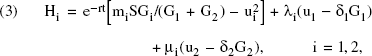
To solve the non–zero-sum differential game described by Equations 1 and 2, we first define the Hamiltonian for firm i:

\begin{matrix} H_{i} = e^{- rt} [m_{i} {SG}_{i} / (G_{1} + G_{2}) - u_{i}^{2}] + λ_{i} (u_{1} - δ_{1} G_{1}) \\ + μ_{i} (u_{2} - δ_{2} G_{2}), i = 1, 2, \end{matrix}

(3)

where λ_i and μ_i are Lagrange multipliers for firm i. We then obtain the open-loop Nash equilibrium solution in which the optimal advertising is a function of time only. This open-loop solution is meaningful from a budgeting standpoint because an advertiser has to commit to a media plan to facilitate the buying of media time and space in advance (for an account of media planning and buying practices, see Abe 1997). However, this solution may not be useful in deciding the best competitive response, which requires a closed-loop solution that is a function of the competitive spending strategy. In the next subsection we obtain expressions for optimal advertising spending and profit in terms of model parameters r, δ_i, and m_i.

Optimal Advertising Spending Level and Profit

After maximizing the Hamiltonians in Equation 3 with respect to u_i, we obtain open-loop solutions, u_i^*(t). These solutions constitute optimal advertising time paths that satisfy the following dynamic system for both firms i ≠ j, i, j = 1, 2 (for details, see Tapiero 1979, p. 912):

\begin{matrix} \frac{{du}_{i}^{*}}{dt} = (δ_{i} + r) u_{i}^{*} (t) - \frac{m_{i} {SG}_{j}}{2 {(G_{1} + G_{2})}^{2}} \\ \frac{{dG}_{i}}{dt} = u_{i}^{*} (t) - δ_{i} G_{i} (t), \end{matrix}

(4)

with initial G_i(0) = G_i0. Observing Equation 4, we find it interesting that each firm's optimal advertising spending depends on the other firm's goodwill, even though the two firms' goodwill dynamics are not interrelated.

In the steady state, all time derivatives vanish. Hence we can set the right-hand side of each part of Equation 4 to zero to obtain the equilibrium quantities ū_i^* and Γ_i as follows:

\begin{matrix} {\bar{u}}_{i}^{*} = \frac{m_{i} S {\bar{G}}_{j}}{2 (δ_{i} + r) {({\bar{G}}_{1} + {\bar{G}}_{2})}^{2}} = δ_{i} {\bar{G}}_{i}, \\ i \neq j, i, j = 1, 2. \end{matrix}

(5)

Because each firm's sales are assumed to be proportional to the share of goodwill, the total market sales are proportional to total goodwill. That is, we assume that S = k(G₁ + G₂), where k is a constant of proportionality. This enables us to simplify Equation 5 further, and the resulting expression for the optimal equilibrium advertising spending by firm i, in terms of model parameters, is

{\bar{u}}_{i}^{*} = \frac{g_{i}}{2 (δ_{i} + r)} \frac{\sqrt{δ_{i} (δ_{i} + r)}}{\sqrt{δ_{1} (δ_{1} + r) + \sqrt{δ_{2} (δ_{2} + r)}}},

(6a)

where g_i (= m_ik) is a constant. Analogously, the profit π_i = m_iSG_i/(G₁+ G₂) - u²_i can be written as

\begin{matrix} {\bar{π}}_{i}^{*} = \frac{m_{i} S {\bar{u}}_{i}^{*} δ_{j}}{{\bar{u}}_{1}^{*} δ_{2} + {\bar{u}}_{2}^{*} δ_{1}} - {({\bar{u}}_{i}^{*})}^{2}, & i \neq j, & i, j = 1, 2 \end{matrix} .

(6b)

Effects of Parameter Bias on Optimal Advertising Spending and Profit

If we suppose the difference between the estimated ${\hat{δ}}_{i}$ and the true parameter δ_i is α (i.e., ${\hat{δ}}_{i} = δ_{i} + α$ ), advertising budget computed from Equation 6a, ${\hat{\bar{u}}}_{i}^{*} = {\bar{u}}_{i}^{*} ({\hat{δ}}_{1}, {\hat{δ}}_{2})$ , is biased. In Appendix A, we show that $\partial {\hat{\bar{u}}}_{i}^{*} / \partial α < 0$ and $\partial {\hat{\bar{π}}}_{i}^{*} / \partial α > 0$ when δ₁ = δ₂. This means that the estimated optimal advertising spending will be understated (overstated) as the positive (negative) bias in ${\hat{δ}}_{1}$ increases in Nerlove–Arrow duopolistic advertising competition. Also, the estimated profit will be overstated (understated) as the positive (negative) bias in ${\hat{δ}}_{1}$ increases. These results hold for both firms. For the case in which δ₁ ≠ δ₂, Monte Carlo findings support these results (see the subsequent section “Simulation Studies”).

In general, parameter bias due to measurement errors in variables is ubiquitous in marketing research. In particular, commercially available advertising data such as awareness, attitude, recall, and GRPs are likely to contain measurement errors. Given the effects of parameter biases on advertising spending and profit, it is important for advertisers to be able to control measurement errors systematically. To achieve this goal, we propose two new methods to remove noise from advertising data.

New Estimators to Control Measurement Errors

We first state the model structure and describe the commonly used OLS and EIV estimators. We then develop two new estimators to control measurement errors in dynamic models.

Model Structure

Let A_it be the awareness measure for goodwill variable G_it, and let x_it denote the GRPs that serve as a measure of spending rate u_it. The model, which includes measurement errors in advertising variables, is

\begin{matrix} A_{it} = G_{it} + ν_{it}, & ν_{it} \sim N (0, σ_{νi}^{2}), \end{matrix}

(7a)

\begin{matrix} x_{it} = u_{it} + η_{it}, & η_{it} \sim N (0, σ_{ηi}^{2}), \end{matrix}

(7b)

and

\begin{matrix} G_{it} = (1 - δ_{i}) G_{i, t - 1} + β_{i} u_{it} + ε_{it}, & ε_{it} \sim N (0, σ_{εi}^{2}), \end{matrix}

(8)

where i = 1, 2, and t = 1, …, T Equation 7 states that observed = true + error as in Morrison and Silva-Risso's (1995) study. All error terms (ε_1t, ε_2t, v_1t, v_2t, η_1t, η_2t)′ are independently distributed normal random variables with zero means. (We relax this assumption subsequently to enable estimation of various pattern of correlation among error terms when we develop the MKF.) Equation 8 is a discrete-time version of Equation 1, because empirical observations are made at discrete points in time (e.g., weekly, monthly). In addition, the error term ε_it makes Equation 8 a stochastic difference equation. It can be interpreted as a perturbation of the dynamic model in Equation 1 induced by various factors, such as misspecification of the functional form or the number of lags. Thus, Equation 8 can be viewed as a first-order stochastic approximation to the true dynamics of advertising response.

In the next two subsections we describe the OLS and EIV estimators. We suppress the subscript i because the goodwill dynamics of the two firms are not directly interrelated and the estimation approaches hold for multiple firms.

OLS Estimator

If we let z_t be the lagged awareness A_t - ₁, the linear regression model for Equation 8 is

A_{t} = (1 - δ) Z_{t} + {βx}_{t} + ε_{t},

(9)

where ε_t ∼ N(0, σ_ε².) for t = 1, …, T. This model ignores the presence of measurement errors (v_t, η_t)′. The resulting 2 × 1 vector of parameters, Θ = [(1 - δ),β]', is estimated by OLS as ${\hat{Θ}}_{OLS} = (X^{'} X) - 1 X^{'} A$ , where matrix X = (z, x), vectors z = (z₁, …, z_n)′, x = (x₁, …, x_n)′, and A= (A₁, …, A_n)′. Note that the first rows in both X and A are discarded because the initial value in z, A₀, is unavailable; thus n = T − 1.

EIV Estimator

The previous OLS estimates will be biased if regressors in X are measured with errors, that is, if either σ² or σ²_v is not zero. Therefore we use the maximum likelihood estimator, which incorporates the presence of measurement errors, to estimate the unknown parameters (see Fuller 1987, Theorem 2.3.1):

{\hat{Θ}}_{EIV} = {(M_{xx} - \hat{λ} Ω_{νη})}^{- 1} M_{xy},

(10)

where M_xx = X'X/n, M_xy = X'A/n, $\hat{λ}$ is the smallest root of the determinantal equation |M_zz - λΣ| = 0, M_zz = 1/nΣⁿ_{t = 1} Z'_tZ_t, Z_t= (A_t, z_t, x_t), Σ = diag(σ_v², σ_v², σ_η²), and Ω_vη = diag(σ_v², σ_η²).

Note that the estimator ${\hat{Θ}}_{EIV}$ is the argument that maximizes the likelihood function formed by multiplying the marginal densities of A_t, t = 1, …, T. This implies that the awareness scores, A_t, are independent across time t. However, this assumption is not valid because the explicit intertemporal dependence in A_t has been induced by the goodwill formation model, Equation 1. Therefore, we expect this EIV estimator to be biased because it ignores the dynamic aspect of advertising response, and thus we must consider alternative ways of controlling measurement errors in dynamic models.

DLS Estimator

In this subsection we develop a new estimator based on wavelet theory (see Donoho and Johnstone 1994, 1995). We first explain the idea of denoising data by using wavelets and then describe what a wavelet is, the denoising procedure, and the proposed DLS estimator. The aim is to extract a signal from noisy empirical data. To this end, we first transform the noisy data (signal plus noise) into a set of numbers called the wavelet coefficients. Large wavelet coefficients represent the signal, whereas small coefficients capture noise. By applying a thresholding scheme that “kills” (sets to zero) the small wavelet coefficients (noise), it is possible to recover the noise-free signal. (The interested reader can find a more detailed introduction to wavelets in Hubbard 1996.)

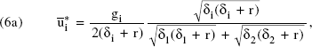
Wavelets

A wavelet is a little wave localized on a compact support that decays quickly to zero everywhere else. Two well-known examples, Haar and Daubechies wavelets, are given in Figure 1. Wavelets theory has been applied successfully to problems in speech recognition, medicine, and image processing (see Aldroubi and Unser 1996; Hubbard 1996; Prasad and Lyengar 1997). One remarkable feature of wavelets is that they are good building block functions for a variety of smooth as well as nonsmooth signals (i.e., sharp bumps, discontinuities, and periodic cycles). This property is especially useful in the context of advertising data because media spending patterns are like square waves of on-and-off pulses (e.g., Mahajan and Muller 1986; Winer 1993), awareness patterns exhibit periodic rise and fall (Zielske 1959), and advertising copy replacement induces sharp jumps (Pekelman and Sethi 1978).

Figure 1

Some Examples of Wavelets

Denoising

Consider the observed GRPs sequence (x₁, …, x_T)′ in Equation 7b. A vector of wavelet coefficients, w, is obtained by applying the discrete wavelet transform to the noisy data vector x = (x₁, …, x_T)′ as follows:

w = Wx,

(11)

where W is a T x T matrix whose elements depend on the specific wavelet (e.g., Haar or Daubechies) used as the filter. These wavelet coefficients are contaminated with measurement noise induced by the noisy data x. To remove the noise, we adopt Donoho and Johnstone's (1994, 1995) hard thresholding scheme:

{\hat{w}}_{t} = {\begin{array}{l} 0 & if | w_{t} | < τ \\ w_{t} & if | w_{t} | \geq τ \end{array},

(12)

where τ is a threshold. In Equation 12, the wavelet coefficient w_t (in absolute magnitude) that is smaller than the threshold τ is killed, whereas the larger coefficient is retained because it contains the signal. The resulting wavelet coefficient $\hat{w}$ is considered noise free. Then we apply the inverse wavelet transform to the vector $\hat{w} = ({\hat{w}}_{1}, \dots, {\hat{w}}_{T})'$ to obtain an estimate of the true signal:

\hat{x} = W^{- 1} \hat{w} .

(13)

Here $\hat{x}$ represents the denoised data because $\hat{w}$ is noise free. We use Donoho and Johnstone's universal threshold τ = λ√2LogT, although various other thresholding options are available (see, e.g., Hurvich and Tsai 1998). To estimate threshold x, we use the standard deviation of the finest detail coefficients as an estimate of the scale parameter λ (for details, see Bruce and Gao 1996, p. 99).

DLS Estimator

In this approach, we first apply the previous denoising procedure to both the dependent and independent variables. We then fit the denoised data with the classic regression model, and we define the resulting estimator as the DLS estimator, ${\hat{Θ}}_{D L S} = {({\hat{X}}^{'} \hat{X})}^{- 1} {\hat{X}}^{'} \hat{A}$ , where $\hat{X}$ contains denoised regressors ẑ and $\hat{x}$ , and Â is the denoised dependent variable. Recently, Cai, Naik, and Tsai (1997) have shown that DLS estimators are consistent and asymptotically unbiased. These properties also hold when the data are denoised using kernel, spline, and other smoothing techniques.

MKF Estimator

This subsection develops a new estimator based on Kalman filtering theory (e.g., Harvey 1994). The proposed estimator is referred to as an MKF, because we allow the independent variable in the standard Kalman filter to be a random variable due to the presence of measurement errors. In other words, we extend the standard Kalman filter to the case of stochastic regressors. Furthermore, the MKF estimator can estimate the correlation between measurement errors as well as the inertia in managerial spending decisions,² which we model next.

We thank two anonymous reviewers for suggesting these two extensions.

Adopting Dekimpe and Hanssens's (1995) approach, we model inertia in spending decisions as a first-order autoregressive, AR(1), process:

\begin{matrix} u_{it} = γ_{i} + ϕ_{i} u_{i t - 1} + a_{it}, & a_{it} \sim N (0, σ_{ai}^{2}), & i = 1, 2. \end{matrix}

(14)

In Equation 14, by suppressing i, we obtain a constant spending pattern (u_t = u_{t − 1} =… = u₀) if ϕ = 1 and γ = σ_a = 0; a random walk (i.e., the persistence effect, as described by Dekimpe and Hanssens [1995]) if ϕ = 1, σ_a ≠ 0, and γ = 0; a random walk with a trend if ϕ = 1, σ_a ≠ 0, and γ ≠ 0; and a simple AR(1) if |ϕ| < 1 and σ_a ≠ 0 regardless of γ. Analogous to Equation 8, Equation 14 is to be viewed as a first-order stochastic approximation to the true temporal spending decisions.

To obtain the MKF estimates, we first express the set of Equations 7, 8, and 14 in a state-space form and then maximize the resulting likelihood function. As in Naik, Mantrala, and Sawyer's (1998) study, we determine the state-space form by deriving the observation and transition equations (see Appendix B for details). For each firm, the observation equation is

[\begin{array}{l} A_{t} \\ x_{t} \end{array}] = [\begin{array}{l} 1 & β \\ 0 & 1 \end{array}] [\begin{array}{l} {\tilde{G}}_{t} \\ {\tilde{u}}_{t} \end{array}] + [\begin{matrix} βγ \\ γ \end{matrix}] + [\begin{array}{l} 1 & β & 1 & 0 \\ 0 & 1 & 0 & 1 \end{array}] [\begin{array}{l} ε_{t} \\ a_{t} \\ ν_{t} \\ η_{t} \end{array}],

(15)

where $\tilde{G} = (1 - δ) G_{t - 1}$ , and (ε_t, a_t, v_t, η_t)′ are normally distributed with mean zeros and covariance matrix H_{4 × 4}. The transition equation is

\begin{matrix} [\begin{array}{l} {\tilde{G}}_{t + 1} \\ {\tilde{u}}_{t + 1} \end{array}] = [\begin{matrix} 1 - δ & β (1 - δ) \\ 0 & ϕ \end{matrix}] [\begin{array}{l} {\tilde{G}}_{t} \\ {\tilde{u}}_{t} \end{array}] + [\begin{matrix} β (1 - δ) γ \\ ϕ γ \end{matrix}], \\ + [\begin{matrix} 1 - δ & β (1 - δ) \\ 0 & ϕ \end{matrix}] [\begin{array}{l} ε_{t} \\ a_{t} \end{array}], \end{matrix}

(16)

where ũ_t = ϕu_{t − 1}, and (ε_t, a_t)′ are normally distributed with mean zeros and covariance matrix Q_{2 × 2}.

The previous state-space form expresses all error terms in the observation Equation 15, which thereby enables the estimation of correlation among error terms (ε_t, a_t, v_t, η_t)′ by properly specifying off-diagonal elements of the covariance matrix H_{4 × 4}. For example, we can estimate the correlation between measurement errors in awareness and GRPs, ρ_vη, by parameterizing the elements (3, 4) and (4, 3) in the matrix H_{4 × 4} with a proper range constraint. The section “An Empirical Example” illustrates this process.

To obtain the likelihood function of the parameter vector θ = (β, δ, ϕ, γ, σ, σ²_a, σ², σ_η², ρ_vη, μ₀)′, we first consider the joint density, g(Y; θ), of the observed advertising data Y = (Y₁, …, Y_T)′, where Y_t = (A_t, x_t)′, A_t is the awareness score, and x_t is the GRPs per week. We then decompose the joint density as a product of the conditional density and the marginal density; that is, g(Y; θ) = f(Y_T|I_{T– 1}) g(Y₁, …, Y_{T– 1}; θ). Here f(Y_T|I_{T– 1}) denotes the conditional density of observing Y_T given the information set IT- 1. The information set contains the history of all information until the realization of advertising data Y_t in the current period; that is, I_t–1 = (Y₁,…, Y_t–1)′. We recursively apply this decomposition so that the likelihood function, L(θ; Y), can be expressed as follows:

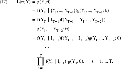
\begin{array}{l} L (θ; Y) & = & g (Y; θ) \\ = & f (Y_{T} | {Y_{1}, …, Y_{T - 1}}) g (Y_{1}, …, Y_{T - 1}; θ) \\ = & f (Y_{T} | I_{T - 1}) f (Y_{T - 1} | {Y_{1}, …, Y_{T - 2}}) \\ g (Y_{1}, …, Y_{T - 2}; θ) \\ = & f (Y_{T} | I_{T - 1}) f (Y_{T - 1} | I_{T - 2}) g (Y_{1}, …, Y_{T - 2}; θ) \\ = & \dots \\ = & \prod_{t = 1}^{T} f (Y_{t} | I_{t - 1}) g (Y_{0}; θ), t = 1, …. T, \end{array}

(17)

where the initial density g(Y₀) is assumed to be normal with mean μ₀. Appendix C shows that the conditional density f(Y_t|I_{t − 1}) is normal for all t and the conditional moments can be expressed as recursive closed forms.

The MKF estimator, ${\hat{θ}}_{M K F}$ , is the argument that maximizes the likelihood function L(θ;Y) in Equation 17. See Appendix C for further details. It can be shown that the MKF estimator is consistent and asymptotically unbiased (e.g., Harvey 1994, p. 128). In addition, any continuous function of this estimator is also asymptotically unbiased because of the invariance property of the maximum likelihood estimators (Mood, Graybill, and Boes 1974, p. 284). Hence, advertisers can determine unbiased optimal advertising spending even though advertising variables are measured with error.

Simulation Studies

This section presents simulation studies³ that compare the performance of four estimators, OLS, EIV, DLS, and MKF, in the ability to estimate true model parameters as measurement noise increases. We first describe the simulation settings, and then we discuss our findings.

We are grateful to an anonymous reviewer for the valuable suggestion of using simulated data.

Simulation Settings

We assumed true parameter values of δ₁ = .05, δ₂ = .10, β₁ = β₂ = 1, ρ = .1, m_iS = 1, g_i = .1, ϕ_i = 1, γ_i = 0, σ_ai = 0 for both firms, and T = 64 observations. Using Equation 6a, we obtained the equilibrium quantities ū^*₁ = 1.26 and ū^*₂ = 1.55. The observed advertising data was constructed by using Equation 7b, x_it = ū^*₁ + η_it, for t = 1, …, T, where the η_it were randomly generated from the normal distribution with mean zero and variance σ_η². Although the variance of measurement noise was the same for both firms (σ_η1 = σ_η2 = σ_η), the scaled measurement noise, σ_η/ū₁^*, will be different for i = 1, 2. The parameter σ_η was varied from .08 to .2 in increments of .01 for moderate noise levels and was set at .25, .33, .5, and .75 for high noise levels. Consequently, the scaled measurement noise ranged from less than 5% to more than 50% for both firms. At high levels of noise some x_it values become negative, and these were replaced by zeros. Finally, goodwill variables were simulated by using Equation 8. Because the average goodwill was about ten times the mean advertising level, the variance of measurement noise of awareness scores in Equation 7a was kept at σ_εi = 10σ_η. This simulated data on awareness and advertising spending was used to estimate model parameters (β_i, δ_i), i = 1, 2. One thousand random realizations generated as many different data sets, and we estimated model parameters for each data set by using the four estimators. We computed DLS estimates by using the Haar wavelet to filter GRPs data and Daubechies wavelet order 4 to filter awareness data (see Figure 1). The findings in the next two subsections are based on the average of these 1000 parameter estimates.

Parameter Biases

In Figure 2, Panel A, we present the OLS, EIV, DLS, and MKF estimates of Firm 1's forgetting rate parameter δ₁. At zero measurement noise, all four estimates are equal to the true one, δ₁ = .05. As measurement noise increases, the estimated parameters tend to depart from the true value. The bias of ${\hat{δ}}_{O L S}$ increases almost linearly, and the bias of d _EIV is not stable. In addition, d_DLS outperforms both OLS and EIV estimates, because it is closer to the true parameter value. However, the DLS estimate begins to deteriorate as the measurement noise goes beyond 20% of the mean advertising level. This may be because the DLS estimator does not account for the dynamics of advertising response. In contrast, ${\hat{δ}}_{M K F}$ is very close to the true parameter value, .05, across the whole range of the scaled measurement noise level. The small bias in d_MKF is due to small sample sizes as well as the nonnormality of x_it (because we replace the negative x_it values with zeros). The MKF estimator performs best.

Figure 2

PARAMETER ESTIMATES

In Figure 2, Panel B, we present the OLS, EIV, DLS, and MKF estimates of the advertising effectiveness parameter β₁. Noting that the EIV estimates are unreasonably large, we scaled them by a factor of 100 so that the four estimates can be plotted together effectively. The patterns of these estimates are essentially similar to those described previously. Because all the results noted also hold for the second firm, the figures for the second firm are not presented here.

Bias in Advertising Spending and Profit

As discussed previously, the estimate of advertising effectiveness may not be equal to its true value, β_i = 1 for i = 1, 2. When this is the case, advertising spending is still given by Equation 6a, whereas the profit expression in Equation 6b becomes ${\bar{π}}_{i}^{*} = (m_{i} S β_{i} {\bar{u}}_{i}^{*} δ_{j}) / (β_{i} {\bar{u}}_{i}^{*} δ_{2} + β_{2} {\bar{u}}_{2}^{*} δ_{1}) - {({\bar{u}}_{i}^{*})}^{2}$ . In Figure 3, Panels A and B, we present the percentage bias in optimal advertising spending and profit, respectively.

Figure 3

EFFECTS OF MEASUREMENT ERRORS

As measurement noise increases, OLS, EIV, DLS, and MKF parameter estimates show upward bias (see Figure 2, Panel A), which leads to a downward bias in advertising spending (see Figure 3, Panel A) and an upward bias in profit (see Figure 3, Panel B). Thus, these simulation findings show that the analytical results (see Appendix A) hold for the case δ₁ ≠ δ₂. Furthermore, even small parameter biases (e.g., MKF estimates) can have a large impact on the estimated advertising spending and profit, which suggests that the optimal advertising spending and profit are sensitive to the presence of measurement errors.

Overall, we find that both OLS and EIV estimators are substantially biased. The parameter biases result in under- or overstating the advertising budget and profit. Therefore, these existing approaches are not adequate to estimate dynamic advertising models when data are noisy. In contrast, the proposed DLS and MKF estimators outperform them. Specifically, DLS reduces the bias, whereas MKF eliminates it asymptotically. Moreover, when measurement noise is moderate, both DLS and MKF estimate the true parameters equally well. As measurement noise becomes large, the MKF estimate stays closer to the true parameter than does the DLS estimate.

From these results we observe that EIV is outperformed by the other three estimators, and therefore it should not be used to estimate dynamic models when data are noisy. DLS is better than OLS and performs as well as the asymptotically unbiased MKF for low to moderate noise levels (noise-to-signal ratio < 20%). MKF is ideal for higher noise levels. Given these results, we next apply DLS and MKF estimators to real advertising data.

An Empircal Example

In this section, we show how advertisers can determine the extent of measurement noise in commercial advertising data. We first briefly describe the advertising data used and then present estimation results.

Figure 4

An Advertising Tracking Study

Data

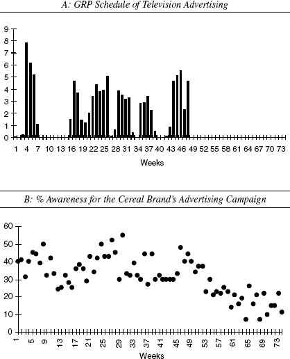
We consider the tracking study of an advertising campaign for a major cereal brand over a period of 74 weeks (for details, see West and Harrison 1997). To illustrate how to determine measurement noise level empirically, we analyze the awareness tracking data for a single firm. The single-firm analysis is appropriate because the goodwill dynamics for the two firms in Equation 1 are not directly interrelated. Figure 4, Panel A, shows the GRPs of television advertising for this cereal brand. Figure 4, Panel B, displays the percentage of survey respondents aware of the brand's advertising during this period. We briefly note here that continuous tracking of advertisements has become the fastest-growing market research technique in the United States (Rossiter and Percy 1997, p. 607), because advertisers are increasingly using such data in advertising decision making. Our proposed methods can complement this desirable development in the practice of advertising.

Estimation Results

DLS estimate of measurement noise level

We first de-noise the GRP data, {x_t}, using the Haar wavelet, and the awareness data, {A_t}, using the Daubechies wavelet of order 2.⁴ Then we apply the standard OLS approach to the resulting denoised data, {Â_t} and { ${\hat{x}}_{t}$ }, to estimate the parameters of the linear models given by Equations 8 and 14. To obtain the extent of noise in awareness data, we compute the standard deviation of the measurement error ${\hat{v}}_{t} = A_{t} - {\hat{A}}_{t}$ , which is estimated as ${\hat{σ}}_{ν} = 4.12$ . Similarly, the GRP noise level is estimated as ${\hat{σ}}_{η} = 3.36$ , which is the standard deviation of the measurement error ${\hat{η}}_{t} = x_{t} - {\hat{x}}_{t}$ .

We tried different orders of Daubechies wavelet to denoise the awareness and GRP data and obtained essentially similar results. It appears from our experimentation that matching the shape of a wavelet with the underlying data pattern is a reasonable heuristic for deciding which wavelet to use as the filter. Thus, our choice was driven by the fact that the shape of a Haar wavelet resembles the square-wave pattern of pulsing media schedules (see Mahajan and Muller 1986), whereas that of a Daubechies 2 wavelet matches the growth and decay in the awareness data (see Zielske 1959). However, we emphasize that the choice of a specific wavelet or even the filtering approach (e.g., wavelet, spline, smoothing) is not crucial because the resulting estimates across these methods are asymptotically unbiased (see Cai, Naik, and Tsai 1997).

To assess whether the measurement noise level is small or large, we compute the noise-to-signal ratio, which is equal to the standard deviation of noise divided by that of the de-noised signal. For the awareness data, noise-to-signal ratio is ${\hat{σ}}_{ν} / {\hat{σ}}_{\hat{A}} = 4.12 / 10.21 = 40.35 %$ , which is indeed quite high. This is because the sample size used in such awareness tracking studies is small; for example, only 66 respondents were surveyed for this brand's advertising (West and Harrison 1997, p. 544). For GRP data the noise-to-signal ratio is ${\hat{σ}}_{η} / {\hat{σ}}_{\hat{x}} = 3.36 / 19.75 = 17.01 %$ , which may be considered moderate. By computing the noise-to-signal ratios, the DLS approach enables advertisers to determine the extent of measurement noise in the empirical data.

Because the noise-to-signal ratio of awareness data is high, the MKF approach must be considered. For the purpose of comparison, we also obtain DLS parameter estimates (see Table 1). A detailed discussion of the DLS and MKF estimates is given next.

Table 1

Empirical Estimates from DLS and MKF Estimators

	DLS		MKF
Parameters	Estimate	t-Value	Estimate	t-Value
Advertising effectiveness, β	.0945	2.72	.1216	7.43
Forgetting rate, δ	.0653	36.6	.0703	7.70
Inertia, ϕ	.6562	7.33	.6450	7.22
Intercept, γ	4.9464	2.26	8.1476	4.15
Measurement noise in awareness, σ_v	4.1157	NTS^a: 40.35%	5.4825	10.35
Measurement noise in GRPs, σ_η	3.3561	NTS: 17.01%	1.1432	.63
Estimation parameter for correlation, κ			10.637	.016

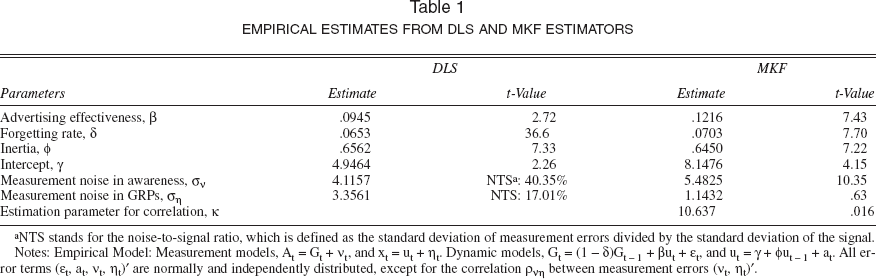
NTS stands for the noise-to-signal ratio, which is defined as the standard deviation of measurement errors divided by the standard deviation of the signal.

Notes: Empirical Model: Measurement models, A_t = G_t + v_t, and x_t = u_t + η_t. Dynamic models, G_t = (1 - δ)G_{t − 1} + βu_t + ε_t, and u_t = γ + ϕu_{t − 1} + a_t. All error terms (ε_t, a_t, v_t, η_t)′ are normally and independently distributed, except for the correlation ρ_vη between measurement errors (v_t, η_t)′.

MKF estimates

Using the maximum likelihood approach (see Appendix C) we obtain the estimates of model parameters, the extent of measurement noise in awareness and GRPs, and the associated standard errors. In Table 1, we present the parameter estimates and t-values. Comparing the DLS and MKF estimates, we find the similarity in the magnitudes of $\hat{β}, \hat{δ}$ , and $\hat{ϕ}$ striking, especially because the genesis and underpinnings of wavelets and Kalman filtering theories are so different. For example, the estimate of the inertia in spending decision is ${\hat{ϕ}}_{MKF} = .6450$ (standard error = .0893) and ${\hat{ϕ}}_{DLS} = .6562$ (standard error = .0909). In addition, we note that both DLS and MKF provide similar statistical inference on the significance of these estimates. Thus, we reject the null hypothesis, H₀: ϕ = 1 at the 5% significance level, and conclude that there is no persistence effect in spending decisions for this cereal brand.

MKF estimates of measurement noise levels

The MKF estimate of the awareness noise level is ${\hat{σ}}_{ν} = 5.48$ , which is statistically significant (t-value = 10.35). The magnitude is comparable to the DLS estimate of ${\hat{σ}}_{ν} = 4.12$ . The two estimates provide a ballpark figure for the true unknown standard deviation of measurement error in the real empirical data. For the GRP data, the estimated measurement noise level ${\hat{σ}}_{η} = 1.1432$ , which is not statistically significant (t-value = .63). Therefore, a comparison with the DLS estimate of ${\hat{σ}}_{η}$ is not meaningful.

Correlation between measurement errors

To estimate the correlation between measurement errors (v_t, η_t), we set the elements (3, 4) and (4, 3) of the covariance matrix H (see Equation 15) to be ρ_vησ_vσ_η. We appropriately constrain the value of ρ_vη, between ± 1 by estimating a parameter κ ∈ (−∞, ∞) such that ρ_vη, = 2f(κ) − 1, where f(κ) = e^κ/(1+ e^κ). The estimated $\hat{κ} = 10.64$ , standard error = 660.38, and thus the t-value is .016. Consequently, the null hypothesis, H₀: κ = 0, cannot be rejected at the 5% significance level. By using the population value of κ = 0, we find that the correlation ρ_vη = 2f(0) −1 = 0. Hence, we conclude that measurement errors in awareness and GRPs are not correlated for this cereal brand.

Conclusion

Advertising variables such as awareness, attitudes, recall, or GRPs can be measured only approximately. The unreliability of measured variables induces substantial bias in OLS estimates, and therefore it becomes difficult to discern the true effectiveness of advertising when data are noisy. Consequently, advertisers are likely to either under- or overspend on advertising. It is therefore imperative to account for measurement errors when dynamic advertising models are estimated. Although the existing EIV approach incorporates measurement errors into its estimation procedure, it ignores the dynamic aspects of advertising response, and therefore the bias in EIV estimates persists. Thus, these existing approaches are not adequate to control for measurement errors in dynamic advertising models, and therefore we have proposed two new approaches.

The DLS approach uses wavelet shrinkage to remove measurement noise from the data before OLS is applied to estimate parameters. This approach successfully reduces the parameter bias, as is shown in our simulation studies. The MKF approach jointly models the effects of measurement errors as well as the dynamic aspects of advertising response, eliminating the parameter bias asymptotically. We emphasize that these conclusions are valid when advertisers know the correct functional form, proper lag specification, the issues of temporal aggregation, and the distribution of errors; then our procedures take care of the remaining source of bias: presence of measurement errors.

Both approaches can estimate the extent of measurement noise in commercial advertising data. In addition, the MKF approach provides information on the statistical significance of the noise level. However, the DLS approach does not offer such a significance test. This is because the use of wavelets in statistics is a recent development (e.g., the pioneering article by Donoho and Johnstone appeared in 1994). Consequently, asymptotic theory for DLS estimators covers point estimation (Cai, Naik, and Tsai 1997), and the issue of statistical inference needs further investigation.

Guidelines for Using DLS and MKF Estimators

If no measurement noise exists, the use of OLS is appropriate. In practice, because measurement noise is usually present, we recommend that advertisers routinely use the DLS approach because it will perform better than OLS and enable them to estimate the noise-to-signal ratio. If the noise-to-signal ratio is less than 20%, DLS is as effective as MKF; otherwise, the MKF approach is recommended. In any case, the EIV approach is not appropriate for estimating dynamic models when data are noisy.

Advertisers also can use the optimal MKF approach to estimate the extent of measurement noise in empirical data and can use this information to negotiate the pricing of market research information. We emphasize that this endeavor involves a method-based judgment on the quality of data. Therefore, advertisers and/or market research firms may want to seek a second opinion to cross-check the magnitude of estimates and achieve convergent validity (Brinberg and McGrath 1985, p. 122). The availability of multiple methods to permit such analyses is especially valuable when the underlying theories are quite different.⁵ Therefore, DLS plays an important role as a meaningful alternative, especially because we know EIV is biased and is not stable for estimating dynamic advertising models. Thus, in practice, we envisage the use of DLS and MKF approaches in a complementary way.

Sarvary and Parker (1997) show theoretically that two expert opinions are complements rather than substitutes when there is a low correlation between the two sources of information. Here, “expert opinion” is the output from these procedures (DLS, MKF) and the “source of information” is the underlying statistical theory (wavelets, Kalman filtering).

Issues for Further Research

We have focused here on the Nerlove–Arrow dynamics of goodwill formation and the AR(1) model of inertia in spending decisions, consistent with the recent marketing literature (Dekimpe and Hanssens 1995; Naik, Mantrala, and Sawyer 1998). First, future studies may apply the proposed methods to other models of advertising response (e.g., the Lanchester model; see Chintagunta and Vilcassim 1992; Erickson 1991, 1992; Fruchter and Kalish 1997) and managerial spending decisions (e.g., AR[p], ARMA[p,q]). Second, the role of measurement errors in other marketing-mix variables (e.g., price) needs investigation; attraction models provide a useful framework to study this problem (see Cooper and Nakanishi 1988). Third, a significance test for the DLS estimate of measurement noise level is required. Fourth, theoretical properties of MKF estimators when the mean function involves aberrant time series (i.e., cycles, discontinuities, and sharp jumps) need verification. Fifth, the estimation of cointegrated time series models with EIV is an open topic. Sixth, biases due to misspecification of models need investigation (e.g., White 1982).

In conclusion, given the millions of dollars of advertising expenditure, we believe that the potential savings from optimizing the budgeting decision will far outweigh the costs of implementing the proposed methods. We hope that advertisers and market research firms use these approaches to improve their marketing practices.

Footnotes

The Effects of Parameter Bias

This appendix shows the effects of parameter bias on optimal advertising spending and profit. Let α denote the bias in estimating the true forgetting rate δ_i, so that the estimated parameter ${\hat{δ}}_{i} = δ_{i} + α$ . Substituting the estimated values ${\hat{δ}}_{1}$ and ${\hat{δ}}_{2}$ into Equation 6, we obtain the estimated advertising spending ${\hat{\bar{u}}}_{i}^{*}$ and profit ${\hat{\bar{π}}}_{i}^{*}$ for both firms i = 1, 2. For Firm 1, these quantities are

To determine the effect of parameter bias, we examine the signs of $\partial {\hat{\bar{u}}}_{i}^{*} / \partial α$ and $\partial {\hat{\bar{π}}}_{i}^{*} / \partial α$ . To keep the algebra simple, we assume that δ₁ = δ₂ = δ. Then,

Thus, the estimated advertising spending is understated (overstated) and the estimated profit is overstated (understated) as the positive (negative) parameter bias increases. When δ₁ ≠ δ₂, the algebraic expressions for $\partial {\hat{\bar{u}}}_{i}^{*} / \partial α$ and $\partial {\hat{\bar{π}}}_{i}^{*} / \partial α$ are complicated, but simulation studies show that upward (downward) biases in parameters lead to negative (positive) bias in advertising spending and positive (negative) bias in profit (see Figures 2 and 3).

Derivation of the State-Space Form

This appendix shows how to obtain the state-space form, consisting of the observation Equation 15 and transition Equation 16. We suppress the index i for the two firms for the sake of notational simplicity.

To obtain the transition Equation 16, consider the following change of variables:

and

Then we substitute Equations B1 and B2 in model Equations 8 and 14 given in the article, respectively, to get

and

Now lead the Equation B1 by one time period and then substitute Equation B3 in the resulting right-hand side as shown:

Therefore,

Similarly, lead Equation B2 by one time period and substitute Equation B4 in the right-hand side to get

Therefore,

Now substitute Equation B4 into Equation B5 so that the right-hand side is expressed in terms of the new variables. Thus,

We express the Equations B6 and B7 in vector notation as follows:

This equation is the transition Equation 16 given in the article.

To obtain the observation Equation 15, we substitute Equations B3 and B4 in Equation 7a given in the article. Thus, we get

Similarly, we substitute Equation B4 in Equation 7b in the article,

and thus get

We express the Equations B9 and B10 in vector notation as follows:

This equation is the observation Equation 15 given in the article. Thus, together, Equations B8 and B11 constitute the state-space form.

Moments of the Conditional Density f(Y t |I t − 1 )

In this appendix, we show that distribution of Y_t given I_t–1 is normal for all t, then derive the conditional mean and covariance expressions, and finally state the estimation procedure for the MKF estimator.

The observation Equation 15 can be expressed generally as

where

Similarly, the transition Equation 16 can be written as

where

In addition, the error terms ω_t and $ϖ_{t}$ are normally distributed with mean zero and covariance,

where

It is important to note that the matrix S arises because the error terms (ε_t, a_t)′ are common to both the observation and transition equations (i.e., Equations C1 and C2).

To show normality of Y_t|I_{t − 1}, we note that both the observation and transition equations (see Equations C1 and C2) are linear in the state variable α_t and the error terms (ω_t, $ϖ_{t}$ ) are normal (see Equation C3), and then we use the result that the sum of normal random variables is also a normal random variable. Therefore, the random variable Y_t|I_{t − 1} is normally distributed. Next, we derive the moments of the normal random variable Y_t|I_{t − 1}.

Let Ȳ_t and F_t denote the mean and covariance of Y_t|I_t–1, respectively; that is, Y_t|I_t–1 ∼ N(Ȳ_t, F_t). To obtain the mean, we take the conditional expectation of the observation equation:

where a_{t|t − 1} denotes the mean of σ_t given I_{t − 1}, which is to be determined. Similarly, to obtain the covariance of Y_t|I_{t − 1}, we note that

where P_{t|t − 1} denotes the covariance of α_t given I_{t − 1}, which is to be determined. Next, we seek the expressions for obtaining a_{t + 1|t} and P_t+1|t after observing data Y_t. That is, we determine the mean and covariance of state variable α_{t + 1} given information until I_t = Y_t ∪ I_{t − 1}.

Following the standard filtering literature (Lewis 1986, pp. 122–23), we now write the conditional mean and co-variance of α_{t+ 1}|I_t as follows:

where K_t = [TP_t|t - ₁T′ + eSc'][zP_{t|t − 1}z' + cQc']^–1 is the Kalman gain factor. These are known as the Kalman filter recursions, which provide the closed-form expressions to update optimally the prior distribution α_t|I_{t − 1} after the current information Y_t is received.

We initiate the previous recursive process by assuming that a₀ has a diffused prior distribution with mean μ₀; that is, a_{0| − 1} = μ₀, and P_{0| − 1} = cI, where c is a large constant. Then we iterate Equation C6 over t = 1, 2, 3, …, T to obtain a_{t + 1|t} and P_{t + 1|t} from the knowledge of a_{t|t − 1}, P_{t|t − 1}, and observed data Y_t in period t. Next, we obtain the moments of Y_t|I_{t −1} by using Equations C4 and C5. Using the moments of Y_t|I_{t − 1}, we compute the likelihood function given in Equation 17. Maximizing the likelihood function, we obtain the MKF estimates. We also obtain the standard errors of MKF estimates by evaluating the information matrix at the estimated parameter values (see Harvey 1994, p. 140).

References

Abe

Makoto

(1997), “A Household-Level Television Advertising Exposure Model,” Journal of Marketing Research, 34 (August), 394–405.

Aldroubi

Akram

, and Unser

Michael

(1996), Wavelets in Medicine and Biology. New York: CRC Press.

Aykac

Ahmet

, Corstjens

Marcel

, Gautschi

David

, and Horowitz

Ira

(1989), “Estimation Uncertainty and Optimal Advertising Decisions,” Management Science, 35 (January), 42–50.

Brinberg

David

, and McGrath

Joseph E.

(1985), Validity and the Research Process. Newsbury Park, CA: Sage Publications.

Bruce

Andrew

, and Gao

Hong-Ye

(1996), Applied Wavelet Analysis with S-Plus. New York: Springer.

Bultez

Alain V.

, and Naert

Philippe A.

(1979), “Does Lag Structure Really Matter in Optimizing Advertising Expenditures?” Management Science, 25 (May), 454–65.

Cai

Zong Wu

, Naik

Prasad A.

, and Tsai

Chih-Ling

(1997), “Denoised Least Squares Estimators,” Technical Report #1098, Graduate School of Management, University of California, Davis.

Chintagunta

Pradeep K.

, and Vilcassim

Naufel J.

(1992), “An Empirical Investigation of Advertising Strategies in a Dynamic Duopoly,” Management Science, 38 (September), 1230–44.

Clarke

Darral G.

(1976), “Econometric Measurement of the Duration of Advertising Effect on Sales,” Journal of Marketing Research, 13 (November), 345–57.

10.

Cooper

Lee G.

, and Nakanishi

Masao

(1988), Market-Share Analysis: Evaluating Competitive Marketing Effectiveness. Boston: Kluwer Academic Publishers.

11.

Dekimpe

Marnik G.

, and Hanssens

Dominique M.

(1995), “The Persistence of Marketing Effects on Sales,” Marketing Science, 14 (Winter), 1–21.

12.

Donoho

David L.

, and Johnstone

Iain M.

(1994), “Ideal Spatial Adaptation by Wavelet Shrinkage,” Biometrika, 81 (3), 425–55.

13.

Donoho

David L.

, and Johnstone

Iain M.

(1995), “Adapting to Unknown Smoothness via Wavelet Shrinkage,” Journal of the American Statistical Association, 90 (432), 1200–24.

14.

Dorfman

Robert

, and Steiner

Peter O.

(1954), “Optimal Advertising and Optimal Quality,” American Economic Review, 44 (December), 826–36.

15.

Erickson

Gary M.

(1991), Dynamic Models of Advertising Competition. Boston: Kluwer Academic Publishers.

16.

Erickson

Gary M.

(1992), “Empirical Analysis of Closed-Loop Duopoly Advertising Strategies,” Management Science, 38 (December), 1732–49.

17.

Erickson

Gary M.

(1995), “Advertising Strategies in a Dynamic Oligopoly,” Journal of Marketing Research, 32 (May), 233–37.

18.

Feichtinger

Gustav

, Hartl

Richard F.

, and Sethi

Suresh P.

(1994), “Optimal Control Models in Advertising: Recent Developments,” Management Science, 40 (February), 195–226.

19.

Fruchter

Gila E.

, and Kalish

Shlomo

(1997), “Closed-Loop Advertising Strategies in a Duopoly,” Management Science, 43 (January), 54–63.

20.

Fuller

Wayne A.

(1987), Measurement Error Models. New York: John Wiley & Sons.

21.

Harvey

Andrew

(1994), Forecasting, Structural Time Series Models and the Kalman Filter. New York: Cambridge University Press.

22.

Hubbard

Barbara

(1996), The World According to Wavelets: The Story of a Mathematical Technique in the Making. Wellesley, MA: A.K. Peters.

23.

Hurvich

Clifford

, and Tsai

Chih-Ling

(1998), “A Cross-Validatory AIC for Hard Wavelet Thresholding in Spatially Adaptive Function Estimation,” Biometrika, 85 (September), 701–10.

24.

Kimball

George E.

(1957), “Some Industrial Applications of Military Operations Research Methods,” Operations Research, 5 (April), 201–204.

25.

Lehmann

Donald R.

, and Winer

Russell S.

(1997), Product Management, 2d ed. Chicago: Richard D. Irwin.

26.

Lewis

Frank L.

(1986), Optimal Estimation. New York: Wiley-Interscience.

27.

Mahajan

Vijay

, and Muller

Eitan

(1986), “Advertising Pulsing Policies for Generating Awareness for New Products,” Marketing Science, 5 (Spring), 89–111.

28.

Mood

Alexander M.

, Graybill

Franklin A.

, and Boes

Duane C.

(1974), Introduction to the Theory of Statistics, 3d ed. New York: McGraw-Hill.

29.

Morrison

Donald G.

, and Silva-Risso

Jorge

(1995), “A Latent Look at Empirical Generalizations,” Marketing Science, 14 (Summer), G61–G70.

30.

Naik

Prasad A.

, Mantrala

Murali K.

, and Sawyer

Alan G.

(1998), “Planning Media Schedules in the Presence of Dynamic Advertising Quality,” Marketing Science, 17 (3), 214–35.

31.

Nerlove

Marc

, and Arrow

Kenneth

(1962), “Optimal Advertising Policy Under Dynamic Conditions,” Economica, 29 (May), 129–42.

32.

Pekelman

Dov

, and Sethi

Suresh

(1978), “Advertising Budgeting, Wearout and Copy Replacement,” Journal of Operations Research Society, 29 (7), 651–59.

33.

Prasad

, and Lyengar

S.S.

(1997), Wavelets Analysis with Applications to Image Processing. New York: CRC Press.

34.

Rossiter

John R.

, and Percy

Larry

(1997), Advertising Communications and Promotion Management, 2d ed. New York: McGraw-Hill.

35.

Sarvary

Miklos

, and Parker

Philip M.

(1997), “Marketing Information: A Competitive Analysis,” Marketing Science, 16 (1), 24–38.

36.

Tapiero

Charles S.

(1979), “A Generalization of the Nerlove-Arrow Model to Multi-Firms Advertising Under Uncertainty,” Management Science, 25 (September), 907–15.

37.

West

Mike

, and Harrison

Jeff

(1997), Bayesian Forecasting and Dynamic Models, 2d ed. New York: Springer-Verlag.

38.

White

Halbert

(1982), “Maximum Likelihood Estimation of Misspecified Models,” Econometrica, 50 (1), 1–16.

39.

Winer

Russell S.

(1993), “Using Single-Source Scanner Data as a Natural Experiment for Evaluating Advertising Effects,” Journal of Marketing Science, 2 (12), 15–31.

40.

Zielske

H. A.

(1959), “The Remembering and Forgetting of Advertising,” Journal of Marketing, 23 (January), 239–43.