Impact of a Late Entrant on the Diffusion of a New Product/Service

Abstract

Starting with Bass's (1969) article, diffusion researchers have predominantly focused on modeling category-level sales growth and issues surrounding it. In this article, the authors propose a brand-level diffusion model and demonstrate its managerial use by applying it to the following issue: If a new brand enters a category that has not attained its peak sales, how can a practicing manager evaluate its impact on the category and on the incumbent brands? The proposed model helps the manager diagnose whether the late entrant affects the market potential and/or the diffusion speed of the category and of the incumbent brands. The authors test the model using brand-level sales data from the cellular telephone industry in multiple markets.

Following the success of Bass's (1969) model, marketing researchers have been developing many different types of diffusion models to address various issues surrounding the sales growth of new durables. These issues include analyzing the role of price and advertising on diffusion (e.g., Bass, Krishnan, and Jain 1994), deriving the optimal price and advertising paths for a new durable (Horsky 1990; Krishnan, Bass, and Jain 1999), developing intergeneration diffusion (Norton and Bass 1987, 1992), and so forth. A careful analysis of the diffusion literature reveals that most of the diffusion models focus only on category-level diffusion and that there are only a few models that research diffusion at the brand level. For companies such as Intel and Microsoft that hold near-monopoly positions in their respective markets, the category-level sales growth is of primary concern. But in industries such as minivans and cellular telephones, which are marked by severe competition, brand managers are likely to pay equal, if not more, attention to understanding the sales growth at the brand level.

Three possible reasons for the dearth of research in brand-level diffusion are (1) the belief that the theory underlying the diffusion process (i.e., the sociocontagion theory) is most applicable to a category, not to its brands; (2) the fact that the sales of a brand in a new category are affected by multiple factors (such as category-level diffusion, marketing-mix variables such as price and advertising of each brand in the market, and different entry times of the various brands); and (3) the nonavailability of appropriate data to test the models. Perhaps because of these problems, marketing researchers have avoided building a comprehensive brand-level diffusion model. Instead, they have focused on specific issues that characterize a brand's diffusion. For example, Givon, Mahajan, and Muller (1995) study the impact of piracy sales on the diffusion of legal software products and treat the pirated version as another brand whose diffusion is not observed.

Along this tradition, in this article we study a key issue that has not been addressed so far and is of great importance to the practicing new product managers. We want to analyze the impact of a later entrant on the sales growth of the category and of the existing brands. Many product managers face the problems associated with brand-level diffusion. For example, consider the minivan market. DaimlerChrysler introduced the first minivans (Dodge Caravan and Plymouth Voyager) to the market in 1984, and thanks to the immense success, many competing brands came into the market within a few years' time. Ford introduced its Aerostar rather late in the diffusion but was able to capture a sizable portion of the market. In this case, the Caravan/Voyager product manager might want to evaluate what happened to the market and to its own sales because of the entry of other brands. In the case of minivans, about which the consumers are somewhat knowledgeable, the main concern of the product managers is likely to center around the potential effects one brand may have on the diffusion of the other brands. However, in the cellular telephone industry, a category that itself is new to the customer, a critical issue is the effects of the brands' diffusion on the category, and vice versa

In Figure 1, we provide a graphic representation of the quarterly sales growth of a product category and its three brands from a typical market in the United States.¹ As depicted in the graph, when the third brand entered the market in quarter 49, the sales growth of the category and of the two incumbent brands were affected, especially in quarters 49 through 51. However, by looking at this graph, it is hard for the product manager to figure out the exact nature of the impact. In other words, the graph does not explain what actually happened in terms of market expansion, diffusion acceleration of the whole category, and diffusion acceleration/deceleration of the incumbent brands. An analytical model that extracts this information will be of a great help to a product manager.

As can be seen from the graph in Figure 1, the product category is cellular telephone services. For the sake of confidentiality, the sales figures have been altered through a linear transformation, which maintains the general shape of the diffusion curves. Also note that the sales figures are the quarterly adoptions and not the cumulative adoption base.

Figure 1

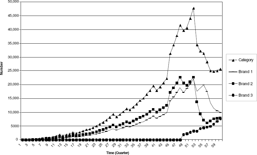
NUMBER OF NEW WIRELESS SUBSCRIBERS IN EACH PERIOD

The article is organized as follows: In the next section, we develop our brand-level diffusion model, compare it with the equivalent models found in the extant literature, and extend it to include the impact of a late entrant. In the following section, we discuss the database on the cellular telephone market that we use in the analysis, empirically fit the proposed model, and discuss the results. In the final section, we conclude the article, giving managerial implications and directions for further research.

A BRAND-LEVEL DIFFUSION MODEL

According to diffusion theory, a new product's sales growth at time t largely depends on the strength of word of mouth from its previous adopters. Similarly, a brand's sales growth should then depend on the extent to which it receives good word of mouth from its own previous adopters. However, there are two brand-level issues. First, it can be expected that a competing brand that also receives good word of mouth is likely to affect the sales of the brand in question, perhaps negatively, especially if both brands target the same customer base. We call this the “intrinsic brand issue.” Second, it is not clear whether the market pool from which a brand draws its customers is specific to that brand or common to all the brands. We call this the “market pool issue.”

Given these two issues, how can the brand-level diffusion be modeled? Researchers have handled this in various ways. For example, Mahajan, Sharma, and Buzzell (MSB) (1993) propose

S_{i} (t) = p_{i} [m_{i} - X_{i} (t)] + q_{i} X_{i} (t) [m - X (t)], i = 1, 2,

(1)

where S_i(t) is the sales of brand i, m_i is the market potential of brand i, X_i is the cumulative sales of brand i up to t, X(t) is the cumulative sales of the category up to t, m is the market potential of the category, and p_i and q_i are the external (innovative) and internal (imitative) influence parameters of the diffusion. In this model, the innovator category of adopters for a given brand comes from the brand-specific market, whereas the imitator category of adopters comes from the total market but is influenced only by its own previous adopters. Thus, the MSB model amounts to assuming away the intrinsic brand issue (i.e., the impact of previous adopters of other brands on a brand),² although with respect to the market pool issue, it makes use of both types of market pools. Mahajan, Sharma, and Buzzell (1993) apply their model to the instant camera market and estimate the impact of the Kodak brand on Polaroid, the pioneer brand.

Mahajan, Sharma, and Buzzell (1993) start with a more elaborate model that has all possible brand interaction effects, but the assumptions they make with respect to some of its parameters result in the reduced model discussed here.

For the purposes of this article, we believe that a model that describes the brand-level diffusion of new categories, such as minivans and cellular telephone service, should be different from the MSB model in the following ways: First, behaviorally speaking, the decision to buy a new product such as a minivan or a cellular telephone is driven mainly by personal factors, such as number of children and their ages, number of hours the consumer spends behind the wheel or on tour, job flexibility, and so forth. Therefore, in these cases the question of “what brand to buy” would be only secondary to the “whether or not to buy the category” question, irrespective of whether the consumer is of the innovator or the imitator type. In contrast, for categories such as sports cars, brand effect may be more predominant than the category effects. Therefore, for categories in which the category effect is likely to dominate, if at time t fractions F₁(t) and F₂(t) of the potential market have adopted Brand 1 and Brand 2, respectively, a potential future adopter for Brand 1 can come from the rest of the whole market, that is, from 1 - F₁(t) -F₂(t). If the category effect does not dominate, a potential adopter for Brand 1 can be expected to come only from 1 -F₁(t) (i.e., as in the first term of Equation 1 of the MSB model), for which the market size will be smaller than that of the whole category. Therefore, for categories in which category effect dominates the adoption decision-making process, the market pool of potential adopters at any time t is 1 - F₁(t) - F₂(t) = 1 - F(t). In effect, we claim that for analyzing a category-level diffusion, the Bass (1969) model, which focuses on f(t)/[1 - F(t)], can be used. In contrast, for analyzing the brand-level diffusion, in which category effect dominates the brand effect in the consumers' buying behavior, f_i(t)/1 - F(t), where f(t) is the p.d.f. of time to adoption of the category and f_i(t) is the p.d.f. of time to adoption of brand i, should be used.

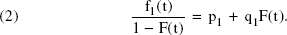
Second, after deciding to buy the category, a potential adopter, say, of a minivan is likely to be swayed by word of mouth about more than one brand available in the market. For a category of two brands, for Brand i (i = 1, 2) the internal influence at time t probably comes from both F₁(t) and F₂(t), with different degrees of influence.³ It is possible, then, to model separately the influence from each brand's previous adopters on a brand's sales. For categories with more than two brands, however, modeling the impact from each brand on a brand's potential sales will make the estimation cumbersome and perhaps unreliable when the data set has only a few observations. What is important to recognize is that each brand is affected by the previous adopters of every brand in the market, that is, by all the previous adopters in the category. Instead of trying to model the influence from each group of previous adopters differently, we can simply note that there exists a collective force of all the previous adopters that act on each brand's future adoption. This collective force is nothing but F(t), the cumulative density function of the time to adopt the category. Because this collective force is the same for all the brands, to ensure that its influence is different on different brands, we employ brand-specific coefficients as follows, for example, for Brand 1:

Each brand's diffusion can be modeled as being affected only by its own previous adopters while drawing adopters from a common pool, as modeled by Mahajan, Sharma, and Buzzell (1993) in the second part of Equation 1. We discuss this approach subsequently in detail.

\frac{f_{1} (t)}{1 - F (t)} = p_{1} + q_{1} F (t) .

(2)

Equation 2 is our proposed model. Two caveats are in order here. First, we implicitly assume that the category in question is well defined. We believe that this assumption is not overly restrictive for categories such as minivans and cellular telephone services. However, if the category boundaries are not well defined, we may need to consider all the products and brands that compete with one another. In those cases, a better model would be Kim, Chang, and Shocker's (1998). Second, brand-level sales can be modeled using the market share formulation. However, for a new consumer durable that is still growing as a category, we believe that the market share model is less appropriate than directly modeling the diffusion. That said, it is important to note that it is easy to derive market share dynamics using the proposed model.

A model similar in spirit to the proposed model has been employed by Givon, Mahajan, and Muller (GMM) (1995) to analyze the extent and the impact of pirated software diffusion on the legal adoption of the product. The model is as follows:

\frac{f_{1} (t)}{1 - F (t)} = p_{1} + {αq}_{l} F (t),

and

\frac{f_{c} (t)}{1 - F (t)} = (1 - α) q_{l} F (t),

where subscript l refers to the legal version and subscript c to the pirated copy version of the software product. Note that 1 - α captures the extent of piracy in the market. Because the adoption data on the pirated version were not observable, the authors use a mathematical algorithm to estimate some of the parameters. Givon, Mahajan, and Muller (1997) extended the GMM (1995) framework to analyze the different growth patterns of the software adopter population and the software user population and to allow brand switching.⁴

A few other researchers have modeled diffusion from a purely normative objective (e.g., Rao and Bass 1985) or an empirical perspective (e.g., Parker and Gatignon 1994).

It is interesting to note that the brand-level models in the extant literature are not solvable so as to yield closed-form solutions. Having a closed-form expression enables researchers to forecast sales for extended periods and carry out “what if” analysis. In this article, we derive an expression for brand-level sales as a function of the time variable alone. Subsequently, we extend the proposed model to capture the impact of a late entrant on the diffusion of the category and of the incumbent brands.

Closed-Form Expression

To derive the closed-form expression for the model expressed in Equation 2, we first derive the category-level model by summing both sides of Equation 2 over all the brands as follows:

\frac{\sum f_{i} (t)}{1 - F (t)} = \sum p_{i} + \sum q_{i} F (t),

(3)

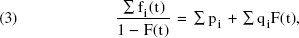
where the summation is done over all the brands in the category. Denoting Σf_i(t) by f_c(t), Σp_i by p, and Σq_i by q, Equation 3 reduces to

\frac{f (t)}{1 - F (t)} = p + qF (t) .

(4)

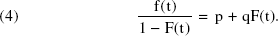
Equation 4 is the category-level model implied by our proposed model. It is easy to see that the model is simply the classic Bass (1969) model. Equation 4 can be solved to yield the following (for details, see Bass 1969):

F (t) = \frac{1 - e^{- (p + q) t}}{1 + (q / p) e^{- (p + q) t}} .

(5)

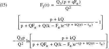
Substituting expression 5 in the brand-level Equation 2 and solving the resulting differential equation, we get

\begin{matrix} F_{i} (t) = \frac{q_{i}}{q} \frac{1 - e^{- (p + q) t}}{1 + (q / p) e^{- (p + q)} t} \\ + \frac{p}{q} (\frac{p_{i}}{p} - \frac{q_{i}}{q}) l n \frac{1 +_{(q / p)}}{1 + (q / p) e^{- (p + q) t}} . \end{matrix}

(6)

Equation 6 expresses the cumulative sales function of Brand 1 as a function of the time variable alone.⁵

The actual derivations mentioned here and elsewhere in the article can be obtained from the first author.

Three points are worth noting here. First, our method of deriving the closed-form expression for brand-level sales from the category-level model is, to the best of our knowledge, a new contribution to the literature. Second, the property that the proposed brand-level model sums up to the Bass (1969) category-level model may look restrictive,⁶ but it gives indirect face validity to the proposed model because the Bass (1969) model has a strong behavioral basis and has found excellent empirical support over a wide range of products (Mahajan, Muller, and Bass 1993). Third, if m denotes the category's market potential, it can be shown that the market potential and the peak sales time of brand i are

Probably for the reason of having to specify certain restrictive assumptions, the authors of the previous studies chose to obviate the need for closed-form solutions. We thank a reviewer for sharing his or her views on this.

m_{i} = {mF}_{i} (\infty) = m \frac{q_{i}}{q} {1 + \frac{p}{q} (\frac{p_{i}}{q} \frac{q}{q_{i}} - 1) ln [1 + (q/p)]},

and

peak sales time of brand i, t_{i}^{*} = \frac{1}{p + q} ln [\frac{2 q_{i} p + q (q_{i} - p_{i})}{p (q_{i} + p_{i})}] .

Noting that the category's peak sales time is 1/(p + q) ln (q/p) (Bass 1969), we show that brand i will reach its peak before the category does if and only if q_i/p_i < q/p. Similarly, we show that brand i will reach its peak earlier than brand j if and only if q_i/p_i < q_j/p_j. A smaller ratio of internal to external force suggests either a poorer word-of-mouth effect and/or a stronger brand equity, both of which lead to an earlier peak sales time but not necessarily a higher peak.

The model formulated thus far assumes that the brands enter the market simultaneously. But in many markets, there are successful late entrants. In the event of a successful late entrant, the managers of incumbent brands will be curious to know exactly how the new entrant will affect the category as a whole, their own brands in particular, and the competing brands. In the next section, we extend the proposed model to answer these questions.

Entry of a New Brand at Time t_n

Suppose that two brands are present in the market from the time of introduction of the category; that is, t = 0. Suppose at time t_n a third brand enters the market, where t_n > 0. One of three things can be expected to happen to the market at the category level. The category will expand (i.e., m will become larger), the category will start diffusing faster (i.e., q will be higher), or both market expansion and faster diffusion will happen simultaneously. At the brand level, the existing brands may get affected in their diffusion speed either positively or negatively, and the exact effect depends on the parameters m, q, and q_i.

We focus on the most general model, that is, one in which the new entry affects both the market potential and the diffusion speed of the category and of the existing brands. For ease of exposition, we assume that Brands 1 and 2 entered the market at t = 0 and Brand 3 entered the market at t = t_n. Let M and Q' represent the market potential and the internal influence coefficient of the category after the third brand entry. Thus, for t > t_n, the category model, in discrete time, is

S (t) = [M - \sum_{t} S (t)] [p + Q' \frac{\sum_{t} S (t)}{M}] .

Denoting M = mk and simplifying the sales equation we get

S (t) = m [k - \frac{\sum_{t} S (t)}{m}] [p + \frac{Q'}{k} \frac{\sum_{t} S (t)}{m}] .

Noting that f(t) = [S(t)/m] = 1/m d/dt [∫S(t)] = d/dt F(t) and then letting Q'/k be Q, we get

\begin{matrix} f (t) = [k - F (t)] [p + QF (t)] & \forall t > t_{n} . \end{matrix}

Similarly, we can derive the diffusion equations for the brands as well. The following differential equations represent the sales growth of the category and the three brands before the third brand entry (i.e., t_n) and after the third brand entry.

\begin{matrix} \frac{f (t)}{1 - F (t)} = p + qF (t), & \forall t \leq t_{n}; \end{matrix}

(7)

\begin{matrix} \frac{f (t)}{k - F (t)} = p + QF (t), & \forall t \geq t_{n}; \end{matrix}

(8)

\begin{matrix} \frac{f_{i} (t)}{1 - F (t)} = p_{i} + q_{i} F (t), & \forall t \leq t_{n}, & i = 1, 2; \end{matrix}

(9)

\begin{matrix} \frac{f_{i} (t)}{k - F (t)} = p_{i} + Q_{i} F (t) & \forall t \geq t_{n}, & i = 1, 2; \end{matrix}

(10)

\begin{matrix} \begin{matrix} f_{3} (t) = 0 & \forall t \leq t_{n} \end{matrix} \end{matrix};

(11)

and

\begin{matrix} \frac{f_{3} (t)}{k - F (t)} = Q_{3} F (t), & \forall t \geq t_{n} \end{matrix} .

(12)

Equations 7 and 8 represent the diffusion of the category before and after the third brand entry, respectively; Equations 9 and 10 represent the diffusion of Brand i (i = 1, 2) before and after the third brand entry; and Equations 11 and 12 represent the diffusion of Brand 3. In Table 1, we present all the notations that we use and estimate in the model.

Table 1

PARAMETERS USED AND ESTIMATED

	Before t_n			After t_n
	Innovation	Imitation	Market Potential	Innovation	Imitation	Market Potential
Category	p	q	m	p	Q	M
Brand 1	p₁	q₁	—	p₁	Q₁	—
Brand 2	p₂	q₂	—	p₂	Q₂	—
Brand 3	—	—	—	—	Q₃	—

In Equations 8, 10, and 12, the parameter k implies that eventually more or less market potential will be realized because of the third brand entry. In other words, F(∞) may have a value different from 1 (to be specific, it will be k, as is shown subsequently), and it is important to realize that though statistically speaking F(∞) should be 1, what we do here is a simple scaling to ensure that the model takes care of the possible market contraction or expansion. Note that we focus our attention on modeling the changes that may occur in the coefficients of imitation (of the category and of the incumbent brands) because of the third brand entry, and thus we let the coefficients of innovation remain unchanged in the process. This helps us study the change in the diffusion speed much more clearly, because in this case we only need to examine the estimates of coefficients of imitation before and after the third brand entry to understand whether the diffusion has speeded up or not. For the same reason, we do not model the coefficient of innovation for the late entrant.

Before we proceed further, a caveat is in order. A new entrant in a market changes the market dynamics not only by its entry but also by the marketing actions and reactions that follow the entry. These actions include price cutting, more advertising and promotional efforts, wider distribution, and so forth, which cause the changes observed in the diffusion dynamics. In this article, we study those changes and not their causes.⁷

If the marketing actions are one-time activities, it may not be possible to diagnose those causes. However, if the firms change their pricing and advertising policies permanently following the third brand entry, it may be possible to analyze those effects using some variation of marketing-mix diffusion models, such as that of Bass, Krishnan, and Jain (1994).

Closed-Form Solutions to the Diffusion Equations

Solutions to Equations 7 and 9 are given by Equations 5 and 6, respectively. To solve the differential Equations 8 and 10, we make use of the fact that the cumulative sales functions are continuous at time t_n. In other words, we first evaluate F(t_n), F_i(t_n) (i = 1, 2) by replacing t by t_n in Equations 5 and 6 and then use those as the initial conditions for solving the corresponding differential Equations 8 and 10 to obtain

F (t) = \frac{k (1 + \frac{Q}{p} F_{n}) - (k - F_{n}) e^{- (p + kQ) (t - t_{n})}}{(1 + \frac{Q}{p} F_{n}) - \frac{Q}{p} (k - F_{n}) e^{- (p + kQ) (t - t_{n})}}

(13)

and

\begin{matrix} F_{i} (t) = F_{in} + \frac{Q_{i} (p + {qF}_{n})}{Q^{2}} \\ [\frac{p + kQ}{p + {QF}_{n} + Q (k - F_{n}) e^{- (p ​ ​ + kQ)}^{(t - t_{n})}} - 1] \\ - \frac{Q_{i} p - p_{i} Q}{Q^{2}} ln [\frac{p + kQ}{p + {QF}_{n} + Q (k - F {}_{n}) e^{- (p + kq) (t - t_{n})}}] . \end{matrix}

(14)

Note that we denote F(t_n) and F_i(t_n) by F_n and F_in, respectively. Equations 13 and 14 describe the cumulative sales growth of the category and of brand i, respectively, after the third brand entry. By letting t = ∞ in Equation 13, we find that F(∞) = k, and because the market potential of the category before the third brand entry is scaled to 1, the estimated value of k will tell us by what percentage the market has expanded or contracted because of the third brand entry. Similarly, by comparing the estimated value of F_i(∞) before and after the third brand entry, we can compute what happened to the market potential of Brand i because of the late entrant. To obtain the cumulative sales function for Brand 3, we recognize that its cumulative sales at t = t_n are 0. Then, similar to Equation 14, which describes the cumulative sales function of Brands 1 and 2 after t_n, the cumulative sales function for Brand 3 can be shown as

\begin{matrix} F_{3} (t) = \frac{Q_{3} (p + {qF}_{n})}{Q^{2}} \\ [\frac{p + kQ}{p + {QF}_{n} + Q (k - F_{n}) e^{- (p + kQ) (t - t_{n})}} - 1] \\ - \frac{Q_{3} p}{Q^{2}} ln [\frac{p + kQ}{p + {QF}_{n} + Q (k - F_{n}) e^{- (p + kQ) (t - t_{n})}}] . \end{matrix}

(15)

The set of equations given by 13, 14, and 15, along with the set of Equations 5, 6, and 11, provides us with the cumulative sales growth of the category, of Brand i (i = 1, 2), and of Brand 3 for the entire duration, that is, from t = 0 to well after t = t_n.

The proposed model can be used for several purposes. For example, by applying these equations to an empirical data set and by comparing the estimates of equivalent parameters before and after the third brand entry, we can infer the changes in the speed of diffusion of the category and of each brand and the changes in the market potential of the category and of each brand. Moreover, because Brand 1 is influenced by the previous adopters of all brands in proportion to their sizes and in turn influences the other brands' future adopters, it is also possible to estimate the net benefits that Brand 1 gets in the process as follows:

\begin{matrix} N e t b e n e f i t s t o b r a n d 1 u p t o \\ t = \sum_{u = 0}^{t} ([1 - F (u)] {q_{1} [F (u) - F_{1} (u)] - \sum_{j \neq 1} q_{j} F_{1} (u)}) . \end{matrix}

Note that in this expression, because the q's change when the third brand enters, appropriate values must be used if t_n is encountered in the period of interest. Also note that this expression can be easily modified and used to estimate the flow of dynamics between any two specific brands for any period of interest.

In this article, for space considerations, we focus only on empirically estimating the changes in the diffusion dynamics of each brand and category occurring because of the third brand entry. We now apply the model on a given data set, and on the basis of the estimates we obtain for k, Q, Q₁, and Q₂, we infer whether the third entry caused the market potential to change or caused the diffusion to hasten/slow down or both. As a null model, we use the following alternative specification that we briefly mentioned in a previous section:⁸

We thank a reviewer for bringing this model to our attention.

f_{i} (t) = [1 - F (t)] [p_{i} + {qF}_{i} (t)],

(16)

where p_i is brand i's coefficient of external influence. Note that Equation 16 adds up (across brands) to the Bass (1969) model f(t) = [1 - F(t)][p + qF(t)], where p = Σp_i. Using this information, we can show that F_i(t) = (p_i/p)F(t). Because this is true for all t, we get f_i(t) = (p_i/p)f(t). Although the alternative model is simple and parsimonious, a disturbing implication is that the market share of brand i—that is, f_i(t)/f(t)— remains a constant across time. The cellular telephone market we analyze is marked by brands whose market shares tend to change considerably over time. Therefore, we expect our proposed model to perform better than the alternative model specification.

Empirical Demonstration

The data for the study were provided by the wireless service providers that have national presence.⁹ These firms operate in many cities (i.e., markets) in the United States. The wireless service was introduced in the United States in 1983, when only two firms were allowed to compete in each market. In 1994, license was granted for the third firm to enter the market. The data were available on a quarterly basis from 1983 until 1996. The data set contains information on the number of new subscribers in each quarter. The subscriber sales did not peak before 1994 in almost all of the markets. Although it is widely acknowledged that the cellular telephone market has been witnessing a “churning” because of brand switching, the data we collected have been cleansed of these elements for the purpose of this study. Data from six markets were used for model estimation.¹⁰

For reasons of confidentiality, we are not able to provide the names of the companies concerned.

The sales data pertaining to one of the three markets is shown in Figure 1. As is discussed in the introduction section, the graph does not explain what happens because of the third brand entry in quarter 49.

Empirical Results and Discussion

We used the quarterly sales data on cellular subscribers explained in the previous section. We fitted the data simultaneously on six equations (two for category, two for Brand 1, two for Brand 2, and one for Brand 3). The sales equation was derived as the difference between two consecutive quarters' cumulative sales equation; that is,

Sales (t) = m \times [Cumulative Sales (t) - Cumulative Sales (t - 1)],

where the cumulative sales functions for category and its three brands, 1, 2, and 3, are given by Equations 5, 6, 11, 13, 14, and 15. We used the SYSNLIN procedure in SAS to estimate the seven equations.

For clarification purposes, we produce in Table 2 the estimation results of Markets 1 and 4, in Table 3 the estimation results of Markets 2 and 5, and in Table 4 the estimation results of Markets 3 and 6. For each market, we have reported for the category, Brand 1, and Brand 2 two sets of estimates of innovation and imitation and market potential, one before the third brand entry and one after the entry; we have reported for Brand 3 the coefficient of imitation.

Table 2

ESTIMATION RESULTS OF MARKETS IN WHICH ONLY DIFFUSION SPEED (I.E., IMITATION COEFFICIENT) CHANGED

Market 1
	Before t_n: Coefficients of			After t_n: Coefficients of
	R-Square	Innovation	Imitation	Market Potential	Imitation	Market Potential
Category	.9303	.000129	.1424	1,112,437	.1708	1,112,437
Brand 1	.9315	.000799	.0614	n.e.	.0853	n.e.
Brand 2	.7936	.001012	.0758	n.e.	.0605	n.e.
Brand 3	.6154	n.a.	n.a.	n.a.	.0202	n.e.

Market 4
	Before t_n: Coefficients of			After t_n: Coefficients of
	R-Square	Innovation	Imitation	Market Potential	Imitation	Market Potential
Category	.9406	.000140	.1526	1,062,812	.1894	1,062,812
Brand 1	.9218	.000310	.0703	n.e.	.0911	n.e.
Brand 2	.8332	.000940	.0810	n.e.	.0723	n.e.
Brand 3	.6496	n.a.	n.a.	n.a.	.0260	n.e.

Notes: All the reported estimates are significant at the 5% level. The notation n.a. means not applicable, and the notation n.e. means not estimated in the model.

Table 3

ESTIMATION RESULTS OF MARKETS IN WHICH ONLY MARKET POTENTIAL CHANGED

Market 2
	Before t_n: Coefficients of			After t_n: Coefficients of
	R-Square	Innovation	Imitation	Market Potential	Imitation	Market Potential
Category	.9274	.000103	.1534	638,313	.1501	689,016
Brand 1	.9188	.000870	.0733	n.e.	.0700	n.e.
Brand 2	.7398	.001819	.0620	n.e.	.0602	n.e.
Brand 3	.6544	n.a.	n.a.	n.a.	.0214	n.e.

Market 5
	Before t_n: Coefficients of			After t_n: Coefficients of
	R-Square	Innovation	Imitation	Market Potential	Imitation	Market Potential
Category	.9091	.000148	.1596	770,414	.1545	841,754
Brand 1	.8944	.000921	.0761	n.e.	.0721	n.e.
Brand 2	.7561	.001347	.0644	n.e.	.0610	n.e.
Brand 3	.6873	n.a.	n.a.	n.a.	.0190	n.e.

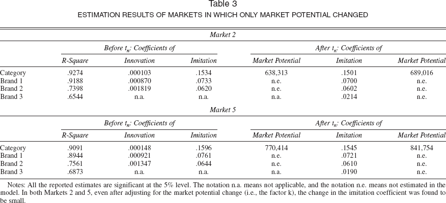
Notes: All the reported estimates are significant at the 5% level. The notation n.a. means not applicable, and the notation n.e. means not estimated in the model. In both Markets 2 and 5, even after adjusting for the market potential change (i.e., the factor k), the change in the imitation coefficient was found to be small.

Table 4

ESTIMATION RESULTS OF MARKETS IN WHICH BOTH DIFFUSION SPEED AND MARKET POTENTIAL CHANGED

Market 3
	Before t_n: Coefficients of			After t_n: Coefficients of
	R-Square	Innovation	Imitation	Market Potential	Imitation	Market Potential
Category	.9368	.00013	.1468	1,358,254	.1934	1,426,267
Brand 1	.9301	.00067	.0694	n.e.	.0974	n.e.
Brand 2	.8106	.0011	.0821	n.e.	.0648	n.e.
Brand 3	.7104	n.a.	n.a.	n.a.	.0312	n.e.

Market 6
	Before t_n: Coefficients of			After t_n: Coefficients of
	R-Square	Innovation	Imitation	Market Potential	Imitation	Market Potential
Category	.9314	.000171	.1588	1,264,589	.1993	1,332,118
Brand 1	.9276	.000740	.0736	n.e.	.0896	n.e.
Brand 2	.8368	.000900	.0847	n.e.	.0788	n.e.
Brand 3	.7457	n.a.	n.a.	n.a.	.0309	n.e.

Notes: All the reported estimates are significant at the 5% level. The notation n.a. means not applicable, and the notation n.e. means not estimated in the model.

Markets 1 and 4 were found to fit best the nested model in which only the diffusion speed and not the market potential was modeled to be affected by the third brand entry. In Market 1 (as reported in Table 2), for example, the market potential remained the same at 1,112,437 units before and after the third brand entry, though the speed of category diffusion represented by the coefficient of imitation increased from .1424 to .1708, roughly a 20% increase. In other words, the marketing activities that followed the third brand entry simply pulled the future buyers to buy the product sooner. The brands that benefited are Brand 1 (whose speed of diffusion—i.e., the coefficient of imitation—increased by 39%, from .0614 to .0853) and Brand 3, whereas Brand 2 seems to have lost its potential future buyers partly to Brand 1 and partly to Brand 3. In other words, the word-of-mouth effect became stronger for Brand 1 and weaker for Brand 2. A similar explanation can be offered for Market 4 in Table 2.

Markets 2 and 5 were found to fit best the nested model in which only the market potential and not the diffusion speed was modeled to be affected by the third brand entry. In Market 2 (as reported in Table 3), the coefficients of imitation remained the same for the category, Brand 1, and Brand 2 before and after the third brand entry, though the market potential increased from 638,313 units to 689,016 units (an increase of approximately 51,000 subscribers) because of the third brand entry. This finding implies that the marketing strategies and activities that followed the third brand entry in this market were able to tap into a new stratum of the socioeconomic structure in the society wherein the word-of-mouth effect remained the same as in the existing market. A similar explanation can be offered for Market 5 in Table 3.

Markets 3 and 6 were found to fit best the comprehensive model in which both the diffusion speed and the market potential were modeled to be affected by the third brand en-try.¹¹ In Market 3 (as reported in Table 4), for example, the speed of the category diffusion represented by the coefficient of imitation increased from .1468 to .1934, roughly a 32% increase, and the market potential increased by 5%, from 1,358,254 units to 1,426,167 units. This market has apparently witnessed such an increased level of marketing activity that not only was a new market tapped into but also the word-of-mouth effect was accelerated. A similar explanation can be offered for Market 6 in Table 4.

We estimated this model in two stages; first, we estimated the model assuming no change in the market potential, and second, we estimated the change in market potential alone. Estimating the model in one stage caused parameter redundancy problems, and the proposed method of fixing m has been used in the diffusion literature by Jain and Rao (1990) and Horsky (1990).

On the basis of our discussion with the brand manager of one of the firms and our own observation, we found that the reason introduction of the third brand opened up the market for additional consumers in Markets 2 and 3 and not in Market 1 is that the subscriber penetration had not reached the lower socioeconomic segment in the former markets, whereas it had done so in the latter market. Another possible reason lies in the specific marketing strategies adopted in the markets.

At the brand level, when Brand 3 entered Market 1 (and Market 3), it practically slowed down the sales growth of Brand 2, whereas the diffusion of Brand 1 was accelerated. In this market, the third brand bought the wireless service from the firm that was marketing Brand 2 and sold it to the customer under a different name. Although the lines were bought by one brand from another, the brands still directly competed with each other in the market and moreover had similar marketing strategies. This is a reason that Brand 2's sales slowed down with the introduction of Brand 3. At the same time, the general increase in the marketing activity helped accelerate the sales growth of Brand 1.

It has been noted by Srinivasan and Mason (1986) and others that the sales data not covering the period up to the peak sales time are likely to result in the nonconvergence of the Bass (1969) model in the estimation stage. To test this, we treated Brand 3 as a separate category and tried estimating its parameters using the prepeak sales data (although we have the data past the peak sales period), and as expected, the nonlinear program did not converge, which indicates that the sales of Brand 3 were not likely to hit their peak any time soon in the diffusion cycle.¹² That means, with data not available past the peak, the sales data of a late entrant, when estimated as a category by itself, are likely to show an excellent growth potential, perhaps beyond the category's peak sales time. However, when we estimated the same prepeak sales data of Brand 3 as a part of the category (i.e., the proposed model) we achieved convergence, which indicates that the category peak sales were controlling Brand 3's sales. This is an important finding, because it shows that brand managers simply cannot afford to neglect what happens at the category level, even if their own brands are having fantastic growth rates. Managers neglecting the category are likely to overestimate their brands' sales growth potential.

It should be noted here that, using the data past peak sales time, we did get convergence for the third brand with the Bass (1969) model.

From the estimates reported on the coefficients of imitation in all three markets, the sum of the brand's imitation coefficients equals the corresponding category imitation coefficient, both before and after the third brand's entry. With respect to the coefficients of innovation, however, the sum of the two brands' innovation coefficients does not equal the corresponding category innovation coefficient. This is because we have forced the innovation coefficient of the third brand to be zero. If we let the third brand have its coefficient of innovation, we get the desired summation result.¹³

In this case, the third brand was found to have a negative innovative coefficient, a reflection of the fact that it had zero sales until its entry into the market. Because this is merely an artifact of the model, we chose to fix it at zero.

We tested the performance of the proposed model against the alternative model discussed in the previous section. We estimated the alternative model using the data from all six markets and found the fit to be poor compared with that of the proposed model. For demonstration purposes, we provide the alternative model's estimates from Markets 1, 2, and 3 in Table 5. Comparing Market 1 in Tables 2 and 5, we find that the proposed model produces a better fit than the alternative model for the category and the brands as well. For example, the R-Squares for the proposed model are .9303 (category), .9315 (Brand 1), .7936 (Brand 2), and .6154 (Brand 3), and for the alternative model, they are .8472 (category), .8519 (Brand 1), .7142 (Brand 2), and .5319 (Brand 3). As explained previously, the relatively poor performance of the alternative model specification probably occurs because the market shares of the brands do not remain constant.

Table 5

ESTIMATION RESULTS OF THE ALTERNATIVE MODEL SPECIFICATION

Market 1
	Before t_n: Coefficients of			After t_n: Coefficients of
	R-Square	Innovation	Imitation	Market Potential	Imitation	Market Potential
Category	.8472	.000144	.1405	1,035,148	.1904	1,035,148
Brand 1	.8519	.000070	.1405	n.e.	.1904	n.e.
Brand 2	.7142	.000065	.1405	n.e.	.1904	n.e.
Brand 3	.5319	.000017	.1405	n.a.	.1904	n.e.

Market 2
	Before t_n: Coefficients of			After t_n: Coefficients of
	R-Square	Innovation	Imitation	Market Potential	Imitation	Market Potential
Category	.8498	.000101	.1500	583,114	.1500	610,458
Brand 1	.8206	.000049	.1500	n.e.	.1500	n.e.
Brand 2	.6526	.000045	.1500	n.e.	.1500	n.e.
Brand 3	.5719	.000012	.1500	n.a.	.1500	n.e.

Market 3
	Before t_n: Coefficients of			After t_n: Coefficients of
	R-Square	Innovation	Imitation	Market Potential	Imitation	Market Potential
Category	.8411	.000120	.1402	1,119,825	.1891	1,125,816
Brand 1	.8568	.000060	.1402	n.e.	.1891	n.e.
Brand 2	.7289	.000050	.1402	n.e.	.1891	n.e.
Brand 3	.6429	.000010	.1402	n.a.	.1891	n.e.

Notes: All the reported estimates are significant at the 5% level. The notation n.a. means not applicable, and the notation n.e. means not estimated in the model.

Forecasting Efficiency

Brand managers are interested in determining how well their brands grow in relation to other brands. Therefore, our objective is to test whether the proposed model, which explicitly models the effect of the third brand entry on the diffusion of the category and of the incumbent brands, does better in terms of forecasting when compared with a model that does not explicitly capture the third brand entry effect. We chose the Bass (1969) model as our reference model, first because to our knowledge there is no equivalent model in the literature that analyzes the effect of a late entrant on the diffusion, and second because the Bass (1969) model has been reported to have excellent predictive capability. To apply the Bass (1969) model, we treated each brand as a category by itself with no interaction with other brands. The holdout sample was the last six quarters of the sales data. The results are provided in Table 6 for all six markets.

Table 6

FORECASTING RESULTS (MAPE)

	Brand 1		Brand 2		Brand 3
	Proposed Model	Null Model	Proposed Model	Null Model	Proposed Model	Null Model
Market 1	2.8%	7.0%	3.1%	8.2%	3.2%	9.6%
Market 2	3.0%	7.8%	2.9%	9.1%	3.7%	10.4%
Market 3	3.9%	9.5%	4.1%	9.8%	4.4%	11.5%
Market 4	3.0%	7.7%	3.4%	7.9%	3.5%	9.3%
Market 5	3.1%	8.2%	3.0%	8.9%	3.6%	9.9%
Market 6	4.2%	10.2%	4.3%	10.8%	4.7%	11.2%

Notes: Markets 1 and 4: Diffusion speed was affected by the third brand entry. Markets 2 and 5: Market potential was affected by the third brand entry. Markets 3 and 6: Both diffusion speed and market potential were affected.

The proposed model is found to have more efficiency in forecasting in terms of lower mean absolute percentage error (MAPE). For example, consider Market 1. The proposed model, which found that the diffusion speed was affected by the third brand entry (see Table 2), yields, on the average, a MAPE of approximately 3% across all three brands, whereas the reference model produces a MAPE of approximately 8% across all three brands.¹⁴ Thus, the forecasting error is reduced substantially with the use of the proposed model.

In this forecasting exercise, the alternative model performed worse than both the proposed model and the null model.

Conclusions and Directions for Further Research

In this article, we developed a brand-level diffusion model and used the framework to analyze the effects of a late entrant on the diffusion dynamics of the category and of the existing brands. We used cellular telephone service adoption data in three markets that showed that in one market the third brand entry increased the market potential of the category, in another market it hastened the speed of diffusion, and in a third market it did both. Our model will be useful to product managers, because a simple graph of the sales data does not explain the complex effect the third brand entry has on the market and the effect the market has on the sales growth of the new brand.

The proposed model has several managerial implications. First, managers can use our model to compare their brands' performance before and after a new brand entry in the market, evaluate their brands' performance with respect to the competing brands, and assess the changes taking place in the diffusion process because of the new brand entry. Second, because we have a closed-form solution, brand managers facing incidents such as the threat of a potential new entrant can develop several “what if” scenarios to understand better the scope of the impact the new entry may have on the market and on their own brands. Third, although our focus was the late-entrant effect, the proposed framework can be used to study the effects of any discrete change in the marketplace, such as a reposition of an existing brand, a major price reduction, and a grand promotional campaign by an existing brand. Our framework can be used to study whether those events achieved the intended goals, and/or what the long-term impacts of such events were.

There are several directions for further research. Although the brand-level modeling is only incidental to studying the impact of a discrete event on the diffusion, different approaches to modeling the brand-level diffusion can be tried. First, modeling the market share for the brands while using the diffusion model for the category is one such approach. Second, because discrete events such as new product entry are always accompanied by promotional campaigns and price reductions, it may be worthwhile to explore how these marketing-mix changes affect the observed changes in the diffusion patterns. Third, it would be interesting to explore what underlying factors drive the market to expand and what factors drive up the diffusion process when a third brand enters the market. For example, research can be directed toward finding out whether the time of entry by a late entrant has any effect on any particular type of market behavior by the incumbent firms and subsequently on this market expansion/diffusion acceleration phenomenon. A useful starting point for this research is the work of Gatignon, Anderson, and Helsen (1989) and Gatignon, Robertson, and Fein (1997). It is also useful to analyze whether and how the various economic characteristics and the social structure of a given market affect the market dynamics for a given product.

References

Bass

Frank M.

(1969), “A New Product Growth Model for Consumer Durables,” Management Science, 15(January), 251–27.

Bass

Frank M.

, Krishnan

Trichy V.

, and Jain

Dipak C.

(1994), “Why the Bass Model Fits Without Decision Variables,” Marketing Science, 13, (Summer), 203–23.

Gatignon

Hubert

, Anderson

Erin

, and Helsen

Kristiaan

(1989), “Competitive Reactions to Market Entry: Explaining Interfirm Differences,” Journal of Marketing Research, 26(1), 44–55.

Gatignon

Hubert

, Anderson

Erin

, Robertson

Thomas S.

, and Fein

Adam J.

(1997), “Incumbent Defense Strategies Against New Product Entry,” International Journal of Research in Marketing, 14(2), 163–76.

Givon

Moshe

, Mahajan

Vijay

, and Muller

Eitan

(1995), “Software Piracy: Estimation of Lost Sales and the Impact on Software Diffusion,” Journal of Marketing, 59(January), 29–37.

Givon

Moshe

, Mahajan

Vijay

, and Muller

Eitan

(1997), “Assessing the Relationship Between the User-Based Market Share and the Unit Sales-Based Market Share for Pirated Software Brands in Competitive Markets,” Technological Forecasting and Social Change, 5(June), 131–44.

Horsky

Dan

(1990), “A Diffusion Model Incorporating Product Benefits, Price, Income and Information,” Marketing Science, 9(Fall), 324–85.

Jain

Dipak

, and Rao

Ram C.

(1990), “Effect of Price on the Demand for Durables: Modeling, Estimation, and Findings,” Journal of Business & Economic Statistics, 8(April), 163–70.

Kim

, Chang

, and Shocker

(1998), “Modeling Inter-category Dynamics for A Growing Information Technology Industry: The Case of Wireless Telecommunications Industry,” working paper, Hong Kong University of Science and Technology.

10.

Krishnan

Trichy V.

, Bass

Frank M.

, and Jain

Dipak C.

(1999), “Optimal Pricing Strategy for New Products,” Management Science, 45(December), 1650–63.

11.

Mahajan

Vijay

, Muller

Eitan

, and Bass

Frank M.

(1993), “New Product Diffusion Models,” in Handbooks in Operations Research and Management Science, Vol. 5, Eliashberg

Jehoshua

, and Lilien

Gary L.

, eds. Amsterdam: North Holland Publishers, 349–408.

12.

Mahajan

Vijay

, Muller

Eitan

, Sharma

Subhash

, and Buzzell

Robert D.

(1993), “Assessing the Impact of Competitive Entry on Market Expansion and Incumbent Sales,” Journal of Marketing, 57(July), 39–52.

13.

Norton

, and Bass

Frank M.

(1987), “A Diffusion Theory Model of Adoption and Substitution of Successive Generations of High Technology Products,” Management Science, 33(September), 1069–86.

14.

Norton

, and Bass

Frank M.

(1992), “Evolution of Technological Generations: The Law of Capture,” Sloan Management Review, 33(Winter), 66–77.

15.

Parker

Philip

, and Gatignon

Hubert

(1994), “Specifying Competitive Effects in Diffusion Models: An Empirical Analysis,” International Journal of Research Marketing, 11(1), 17–39.

16.

Rao

Ram C.

, and Bass

Frank M.

(1985), “Competition, Strategy and Price Dynamics: A Theoretical and Empirical Investigation,” Journal of Marketing Research, 22(August), 283–96.

17.

Srinivasan

, and Mason

C.H.

(1986), “Nonlinear Least Squares Estimation of New Product Diffusion Models,” Marketing Science, 5(Spring), 169–78.

Impact of a Late Entrant on the Diffusion of a New Product/Service

Abstract

A BRAND-LEVEL DIFFUSION MODEL

Closed-Form Expression

Entry of a New Brand at Time tn

Closed-Form Solutions to the Diffusion Equations

Empirical Demonstration

Empirical Results and Discussion

Forecasting Efficiency

Conclusions and Directions for Further Research

References

Entry of a New Brand at Time t_n