The Estimation of Pre- and Postpromotion Dips with Store-Level Scanner Data

Abstract

One of the mysteries of store-level scanner data modeling is the lack of a dip in sales in the weeks following a promotion. Researchers expect to find a postpromotion dip because analyses of household scanner panel data indicate that consumers tend to accelerate their purchases in response to a promotion—that is, they buy earlier and/or purchase larger quantities than they would in the absence of a promotion. Thus, there should also be a pronounced dip in store-level sales in the weeks following a promotion. However, researchers rarely find such dips at either the category or the brand level. Several arguments have been proposed to account for the lack of a postpromotion dip in store-level sales data and to explain why dips may be hidden. Because dips are difficult to detect by traditional models (and by a visual inspection of the data), the authors propose models that can account for a multitude of factors that together cause complex pre- and postpromotion dips. The authors use three alternative distributed lead and lag structures: an Almon model, an unrestricted dynamic effects model, and an exponential decay model. In each model, the authors include four types of price discounts: without any support, with display-only support, with feature-only support, and with feature and display support. The models are calibrated on store-level scanner data for two product categories: tuna and toilet tissue. The authors estimate the dip to be between 4 and 25% of the current sales effect, which is consistent with household-level studies.

One of the key issues in sales promotion research is whether “there is a trough after the deal” (Blattberg, Briesch, and Fox 1995, p. G127). The evidence from analyses of household-level panel data is that consumers accelerate their purchases as a result of sales promotions. For example, Gupta (1988) decomposes the sales effect due to promotion for coffee into brand switching (84%), purchase timing acceleration (14%), and increased purchase quantity (2%). Chiang (1991) obtains similar percentages, and Grover and Srinivasan (1992, pp. 86–87) conclude that “one-fourth of the gain in a week's product category sales resulting from a promotion is at the expense of the succeeding week's sales.” Bell, Chiang, and Padmanabhan (1999) decompose the sales effect for 13 product categories and find that, on average, brand choice accounts for 75% of the total elasticity (range 49%–94%). Thus, the percentage attributable to purchase timing acceleration and increases in purchase quantity varies between 6 and 51%.

At first sight, it might be expected that the acceleration effects in timing and quantity evident at the household level would translate directly into a postpromotion dip in weekly store-level sales data. However, postpromotion dips are rarely detected in visual or (traditional) statistical analyses of store data. A resolution of this paradox is important for both researchers and managers. For researchers, a lack of convergent validity between the results from household-level panel data and weekly store-level sales data casts doubt on the nature of the acceleration phenomenon. Also, many managers say they use store-level (or more highly aggregated) scanner data more frequently for analyses than household-level panel data (Bucklin and Gupta 1999). However, if the household results are accurate, managers who rely on aggregated data for inferences about promotion effects will obtain incorrect conclusions. Unless stockpiling can be properly accounted for, managers will overestimate the effectiveness of promotions: They tend to classify the entire promotion-based sales spike as incremental (Neslin and Schneider Stone 1996). Because managers rely heavily on aggregated data, the most challenging part of the post-promotion dip paradox is the apparent lack of a dip in store-level data. In Figure 1, we show two typical store-level sales graphs from the data used in our empirical application. Neither of these graphs shows any sales dip before or after a sales spike.

Figure 1

Typical Store-Level Sales Graphs

As far as we know, only Doyle and Saunders (1985), Leone (1987), Litvack, Calantone, and Warshaw (1985), and Moriarty (1985) studied acceleration through store data. Doyle and Saunders (1985) demonstrate that lead effects of promotions, resulting from the anticipations of promotions by consumers and other economic agents, can be as important as lagged effects. They examine monthly gas appliance sales as a function of the commission structure for sales personnel and analyze whether salespeople move some customer purchases to the time period in which their commission rates are higher. Doyle and Saunders calculate that approximately 7% of total sales during an eight-week promotion period consisted of sales that would have taken place before the promotion period if commission rates had not been increased during the promotion.

Leone (1987) applies intervention analysis to weekly sales data to evaluate a single “five for $1.00” sale for wet cat food. The weekly sales data graph shows a clear post-promotion dip, and the analyses confirm this dip. Litvack, Calantone, and Warshaw (1985) observe the sales of many items before, during, and after a price cut. The authors do not observe a postpromotion dip in sales for the items that could experience purchase acceleration. Moriarty (1985) includes one-week lagged promotion variables in a sales response function and finds significant postpromotion dips for only 3 of the 15 cases.

Although a few of these studies obtain evidence of pre- or postpromotion dips, Blattberg, Briesch, and Fox (1995, p. G127) mention that “examination of store-level [point-of-service] data for frequently purchased goods rarely reveals a trough after a promotion. This anomaly is surprising and needs to be better understood.” Neslin and Schneider Stone (1996) consider eight possible arguments for the apparent lack of postpromotion dips in store-level sales data. Their arguments imply that the dips may be hidden. As a result, dips will be difficult to detect by traditional models or by a visual inspection of the data. Because brand sales are the aggregate of purchases across (heterogeneous) households, both pre- and postpromotion sales data will have complex patterns. Essentially, sales are shifted from multiple future and past periods into a current, promotion-based sales spike in a nontrivial way.

Neslin and Schneider Stone (1996, p. 92) suggest that researchers carry out “sophisticated distributed lag analyses of weekly sales data in the hopes of measuring the postpromotion dip statistically.” We present a flexible modeling approach and regress brand-level sales on current, lead, and lagged own-brand price indices with three different distributed lead and lag structures: an Almon model, an unrestricted dynamic effects model, and an exponential decay model. We distinguish four types of price discounts: without any support, with feature-only support, with display-only support, and with feature and display support.

The key contributions of our article include the following:

•

We propose a store-level model specification explicitly based on the arguments for the apparent lack of a postpromotion dip in aggregate data.

•

We show that there is no postpromotion dip paradox: We obtain pre- and postpromotion dips that are comparable to those obtained with household data.

•

We propose a new way of modeling the interaction effects between price cuts and various types of support (feature and/or display) and show differences in the magnitude of pre- and postpromotion effects between price cuts with alternative types of support.

In the next section, we briefly review eight arguments for the apparent lack of a postpromotion dip in models of store sales and derive implications from these arguments for the specification of pre- and postpromotion dips. Then we show the model specification and discuss model calibration. We introduce store-level scanner data sets for two product categories and provide empirical evidence for dynamic promotion effects for both categories. Finally, we present our conclusions.

Arguments for the Lack of a Postpromotion Dip and Implications for Model Specification

Neslin and Schneider Stone (1996) provide eight possible arguments for the apparent absence of postpromotion dips in store-level scanner data. Five of their arguments complicate the identification of postpromotion dips in both household-and store-level data:

Consumers purchase deal to deal,

Increased consumption,

Competitive promotions mask the dip,

Positive repeat purchase effects cancel the acceleration effect, and

Retailers partially extend promotions beyond the first week.

We refer to Neslin and Schneider Stone (1996) for a discussion of the first four arguments. We expand on the fifth argument, because it has implications for our model specification. Retailers may extend all or part of a promotion—in particular, display activity—and thereby increase sales immediately after the initial promotion, which will mask the dip (Blattberg and Neslin 1990, p. 358). In principle, this effect can be accounted for with expanded display variables in the model. However, it is possible that extensions are not captured. For example, display activity is measured by weekly store audits, say, on Thursday. If a display is extended only during the first three days of a second week (Monday, Tuesday, and Wednesday), the value of the display variable will not accurately reflect this second week's situation. Therefore, we need lagged display variables to capture this extension effect, which should affect sales positively. The other common scanner data variables (sales, prices, feature activities) do not have this measurement error problem.

The final three arguments provided by Neslin and Schneider Stone (1996) appear to complicate the analysis of store-level data uniquely. They are as follows.

The Combined Effect of Quantity and Timing Acceleration

Time acceleration steals from the weeks immediately following the promotion, depressing sales in those weeks, whereas the effects of quantity stockpiling are manifested during the next consumer purchase occasion, depressing sales often after a lag of a few weeks (Blattberg and Neslin 1990, p. 192). In household-level models, these effects can be measured separately. Our store-level model should account for flexible, multiperiod postpromotion dips to capture these effects jointly.

Lack of Consumer Inventory Sensitivity

Inventory may be reduced to its normal level only after an extended period. Therefore, the postpromotion dip is dissipated into the future. In household-level models, heterogeneity in inventory amounts and sensitivities can be accommodated, whereas a brand sales model should incorporate multiperiod postpromotion dips.

Anticipatory Effects

The literature suggests that consumers form price expectations (Kalwani et al. 1990; Winer 1986). If consumers expect a significant price reduction in the future, they may defer or decelerate their purchases, which causes prepromotion dips. In other words, an expected price decrease in period t may decrease sales in period t − k, k = 1, 2, ….

We assume (cf. Kalwani et al. 1990, Equation 8; Winer 1986) that price expectations are unbiased and that actual prices capture price expectations. Therefore, we propose that sales in period t − k are a function of the actual price in period t. This implies that a retailer that offers a deal in week t will lose sales in week t − k (k ≥ 1) if customers expect a deal to be offered in week t.

Because consumers are heterogeneous in the length of the period they are willing to defer purchases in anticipation of a price promotion, prepromotion dips are spread out over multiple prepromotion weeks. However, we do not know when a prepromotion dip will be the deepest. Therefore, the model should also account for flexible, multiperiod prepromotion dips. We note that household-level models that include future expected prices implicitly account for prepromotion effects.

In summary, the store-level model we want to develop should account for factors that can hide postpromotion dips in traditional store-level models and visual representations of the data. The model should accommodate the following:

Multiple-week, own-brand postpromotion effects that are negative or positive relative to sales under the no-promotion scenario;

Multiple-week, own-brand prepromotion dips;

Flexible pre- and postpromotion effects; and

Current cross-brand effects.

There is limited opportunity to test the relevance of specific arguments on sales data. For example, several arguments can account for the occurrence of negative postpro-motion effects. Thus, we do not propose to test the relevance of any arguments. Instead, our objective is to present and estimate a model that can accommodate complex pre- and postpromotion effects for managerial use and to report the nature and magnitude of these effects in store data.¹

There may be other, relevant differences between models of store sales and models of household purchases that pertain to the differential observability of postpromotion dips. For example, our model does not accommodate store switching. If the sales effect in a given store due to a promotion for a brand in that store partly reflects shifts in sales among stores, the current effect that is potentially incremental to the manufacturer of the brand is overstated. Household models of brand choice typically focus on choices conditional on a product category purchase in any of several stores. If the choice of store is not explicitly modeled, as a function of promotional activities, the household models will be subject to similar problems (for a discussion of the conditions under which household choice models generate the same results as store sales models, see Gupta et al. 1996). Thus, we do not believe there is actually a difference between household- and store-level models on this aspect. Households are unlikely to switch purchases actively between stores as a function of promotions for tuna or tissue, the product categories we study. Store switching tends to occur for such items as soft drinks and disposable diapers (see Kumar and Leone 1988). Other relevant aspects include the following: (1) Household panel data could represent a nonrepresentative sample from store-level data; (2) household data involve the imputation of causal data for items not purchased, whereas store-level data are complete; and (3) the purchases for low-penetration categories may be unreliable with household data.

Model Specification and Calibration

We require a model that accommodates lead and lagged effects for multiple sales promotion variables over multiple weeks in a flexible manner. Basically, there are two approaches: econometric and time series. The econometric approach includes lead and lagged sales promotion variables as predictors in a model of brand sales. The time series approach uses transfer function/intervention modeling. In the latter case, we would use autoregressive integrated moving average models for all variables and estimate a transfer function (if the predictors are continuous) or an intervention model (if the predictors are binary) to relate the criterion variable to the predictors.

The traditional time series approach, used by Leone (1987) and others, must be modified in four ways. First, we have multiple predictors instead of the one used by Leone. Thus, we must model dynamic interactions between the predictors as well. Second, for a given predictor we have multiple promotional observations, whereas Leone evaluates the effect of a single promotion. Third, we need to allow for lead and lagged effects. Although Doyle and Saunders (1985) use time series methods to identify lead and lagged effects for multiple predictors, their final model (see Doyle and Saunders, 1985, p. 59, Equation 3) is an econometric model. Fourth, we have time series observations for multiple stores. We are not aware of transfer function/intervention models for lead and lagged effects of multiple predictors in a pooled data context. Although the development of such models may be a fruitful area for new research, the econometric approach appears to be equally promising and is straightforward to implement.

Our econometric model is a modification of the SCAN^*PRO model (Christen et al. 1997; Foekens, Leeflang, and Wittink 1994; Wittink et al. 1988). The original model includes own- and cross-brand effects of promotions and is estimated with store-level scanner data provided by ACNielsen. It was developed for commercial purposes, and the basic model has been used in more than 1800 different commercial applications in North America, Europe, and Asia. Our modification of the SCAN^*PRo model is related to (1) variable choice and (2) model specification.

Variable Choice

In our model, the criterion variable is the log of unit sales of a brand in a specific store in a given week, as is true for the SCAN^*PRO model. The SCAN^*PRO model includes as predictors four current promotional instruments—discount, feature-only, display-only, and feature and display—for the brand and other brands. We modify this formulation and define (1) own- and cross-brand discounts without support; (2) own- and cross-brand discounts with feature-only support; (3) own- and cross-brand discounts with display-only support; (4) own- and cross-brand discounts with feature and display support; (5) own-brand, feature-only without price cuts; (6) own-brand, display-only without price cuts; and (7) own-brand, feature and display without price cuts.

We specify instruments 1–4 as log price indices. We use logs so that the parameters are elasticities. We use price indices (ratio of actual to regular prices) to capture only the promotional price effects. For instrument 1, we take the log price index observations and multiply them by one for observations with neither feature nor display activity for the brand, and by zero otherwise. The values of instruments 2–4 are determined analogously. We include instruments 5–7 as indicator variables, because there is no price discount associated with those observations. Still, these activities can cause sales increases for the brand (Inman, McAlister, and Hoyer 1990).

Our approach has two advantages over the traditional approach of including log price index variables separately from the indicator variables for the nonprice promotion variables. In our approach, the set of own-brand variables is minimally correlated by definition (as is the set of cross-brand variables), whereas in the traditional approach, the log price index variable is often highly correlated with one or more of the nonprice promotion variables. Also, the interpretation of our results is straightforward: Price cuts are the core of sales promotions, whereas feature and display are communication devices. More important, our variable definitions capture any interaction effects between price cuts and the various types of support, which is one of the key issues in sales promotion research (Blattberg, Briesch, and Fox 1995). Our results show the own- and cross-brand price promotional elasticities for each of the four conditions of support.²

Our approach is somewhat similar to the one followed by Papatla and Krishnamurthi (1996, p. 23, Equation 2). They include interaction effects among indicator variables for price cut dummies, feature, and display. However, their set of predictors is more correlated than our set, and their approach does not generate different price (promotion) elasticities for the promotion conditions.

Our model also includes variables for dynamic price promotion effects. Specifically, we use variables to capture lead and lagged own-brand log price index effects under the four conditions of support.

Model Specification

The current own- and cross-brand variables under promoted conditions are included multiplicatively, as in the SCAN^*PRO model. The lead and lagged own-brand log price indices for the four different conditions are modeled with three alternative dynamic effects specifications:

•

Unrestricted dynamic effects (Judge et al. 1985, pp. 351–56),

•

Exponential decay dynamic effects (a finite duration version of the geometric lag model in Judge et al. 1985, p. 388), and

•

Almon dynamic effects (Judge et al. 1985, pp. 356–64; Stewart 1991, pp. 181–86).

The unrestricted dynamic effects approach approximates lead and lagged effects by including the relevant predictors in lagged (t − 1, t − 2, t − 3, …) as well as lead (t + 1, t + 2, t + 3, …) format. In this specification, all lead and lagged variables have unique parameters. Thus, if criterion variable y_t is explained by current, past, and future values of one predictor variable x_t to a maximum lag of s periods and a maximum lead of s' periods, the unrestricted dynamic effects model is

\begin{matrix} y_{t} = α_{0} + α_{1} x_{t} + \sum_{u = 1}^{s} β_{u} x_{t - u} + \sum_{v = 1}^{s'} γ_{v} x_{t + v} + u_{t}, \\ t = s + 1, …, T - s' . \end{matrix}

(1)

The exponential decay model imposes a structure on the dynamic effects (see also Blattberg and Wisniewski 1989): β_u = λ^u–1 β and γ_v = μ^v–1 γ. As a result, the model with one predictor x_t is

\begin{matrix} y_{t} = α_{0}^{'} + α_{1}^{'} x_{t} + \sum_{u = 1}^{s} λ^{u - 1} {βx}_{t - u} + \sum_{v = 1}^{s'} μ^{v - 1} {γx}_{t + v} + u_{t}^{'}, \\ t = s + 1, …, T - s' . \end{matrix}

(2)

The parameters λ and μ are the decay parameters.

The Almon model approximates the dynamic effects in Equation 1 with polynomials. The lagged effect parameters are β_u = Σ_m^r = ₀ϕ_m(u − 1)^m, r < s (u = 1, …, s).³ The lead effect parameters are γ_v = Σ^r'_m = ₀θ_m(v − 1)^m, r' < s' (v = 1, …, s'). In this manner, the Almon model is

\begin{matrix} y_{t} = α_{0}^{''} + α_{1}^{''} x_{t} + \sum_{u = 1}^{s} \sum_{m = 0}^{r} ϕ_{m} {(u - 1)}^{m} x_{t - u} \\ + \sum_{v = 1}^{s'} \sum_{m = 0}^{r'} θ_{m} {(v - 1)}^{m} x_{t + v} + u_{t}^{''}, t = s + 1, …, T - s' . \end{matrix}

(3)

For u = 1, the first element of this sum is defined as ϕ₀(0)0 ≡ ϕ₀.

Our use of these three alternative dynamic effect specifications differs in three respects from their standard use in the econometric literature. First, our approach includes lead effects as well as lagged effects. Second, instead of modeling the dynamic effects of just one variable, we model the dynamic effects of multiple variables. Third, the standard way researchers use the exponential decay and Almon models is to impose a structure in which the dynamic effect parameters are linked to the current effect parameter. Our approach relaxes this assumption; that is, we let the current effect parameter be estimated independently of the lead and lagged effect parameters, because current price promotion effects are expected to be much larger than (week-specific) lead and lagged effects. In addition, we use separate approaches for lead and lagged effects for all models, because we should incorporate flexible dynamic effects, as mentioned previously. For the exponential decay model, this means that the lagged effect decay parameter λ may differ from the lead effect decay parameter μ. For the Almon model, this means that the degree of the lagged effect polynomial (r) may be different from the degree of the lead effect polynomial (r').

It is clear that the unrestricted dynamic effects approach defined in Equation 1 offers the highest degree of flexibility. However, it involves many lead and lagged effect variables, which may lead to multicollinearity. At the other end is the exponential decay model (Equation 2), which uses few parameters but is relatively inflexible. In Equation 2, the dynamic effect is assumed to be largest in the weeks immediately after (lagged effect) or before (lead effect) the promotion. This may be restrictive because of the multitude of factors causing pre- and postpromotion effects (see the arguments section). The Almon approach (Equation 3) is between these two approaches: It is more flexible than the exponential decay model but more parsimonious than the unrestricted model.⁴

Blattberg and Neslin (1990, p. 190) note that “While there are no published examples of using polynomial lags to measure the lag effects of promotion, the technique appears to be promising.”

For brand k, k = 1, …, J, the full model is

\begin{matrix} In S_{ik, t} & = \sum_{j = 1}^{J} \sum_{ℓ = 1}^{4} α_{jk ℓ} In ({PI}_{ij ℓ, t}) + α_{FK} F_{ik, t} + α_{Dk} D_{ik, t} \\ + α_{FDk} {FD}_{ik, t} + \sum_{u = 1}^{s} \sum_{ℓ = 1}^{4} β_{k ℓ, u} In ({PI}_{ik ℓ, t - u}) \\ + \sum_{v = 1}^{s'} \sum_{ℓ = 1}^{4} γ_{k ℓ, v} In ({PI}_{ik ℓ, t + v}) + ψ_{ik} R_{i} \\ + ξ_{tk} W_{t} + u_{ik,t}, \\ t = s + 1, …, T - s' and i=1, …,N, \end{matrix}

(4)

where the lagged effect parameters β and lead effect parameters γ are kept unrestricted (Equation 1), are modeled as an exponential decay model (Equation 2), or are modeled as an Almon model (Equation 3) and where

ln S_ik,t

is the log unit sales of brand k in store i in week t;

ln(PI_ijℓ,t)

is the log price index (ratio of actual to regular price) of brand j in store i in week t (ℓ = 1 denotes that the observation is supported by neither feature nor display, ℓ = 2 by feature only, ℓ = 3 by display only, and ℓ = 4 by feature and display);

F_ik,t

is a feature-only indicator variable for nonprice promotion observations (F_ik,t = 1 if brand k is featured but not displayed or price promoted by store i in week t, 0 otherwise);

D_ik,t

is a display-only indicator variable for nonprice promotion observations (D_ik,t = 1 if brand k is displayed but not featured or price promoted by store i in week t, 0 otherwise);

FD_ik,t

is an indicator variable for combined use of feature and display for nonprice promotion observations (FD_ik,t = 1 if brand k is featured and displayed but not price promoted by store i in week t, 0 otherwise);

R_i

is a store indicator variable (R_i = 1 if an observation is from store i, 0 otherwise);

W_t

is a weekly indicator variable (W_t = 1 if an observation is from week t, 0 otherwise);

α_jkℓ

is the elasticity of brand k's sales with respect to brand j's price index in the current week (ℓ = 1 denotes that it is supported by neither feature nor display, ℓ = 2 by feature only, ℓ = 3 by display only, and ℓ = 4 by feature and display);

^α_Fk, α_Dk, and α_FDk

are the current-week effects on brand k's log sales resulting from brand k's use of feature only (F), display only (D), and feature and display (FD); each is the effect in the absence of a discount for brand k;

β_kℓ,u

is the elasticity of brand k's sales in week t relative to brand k's price index with support ℓ in week t − u;

γ_kℓ,v

is the elasticity of brand k's sales in week t relative to brand k's price index with support ℓ in week t + v;

ѱ_ik and ξ_tk

are the store intercept for store i (i = 1, …, N), brand k, and the week intercept for week t (t = 1, …, T), brand k, respectively; and

u_ik,t

is a disturbance term for brand k in store i in week t.

Weekly indicator variables are included to account for seasonal effects and the effects of missing variables (e.g., manufacturer advertising, coupons).

This model accounts for the factors that can hide dips, which we presented previously. It includes flexible, multiple-week, pre– and post–price promotion own-brand variables and incorporates current cross-brand price-promotional instruments. Through the use of separate price discount variables for four promotion conditions, the model accommodates lagged price cut with feature effects, which are found to be significant in prior research (Papatla and Krishnamurthi 1996). In summary, the model includes lead and lagged variables for temporary price discounts with four types of support: no support, feature-only, display-only, and feature and display. Thus, our model also accounts for dynamic effects for features and displays (documented also by Lattin and Bucklin 1989), to the extent that these promotions were accompanied by price discounts.⁵

We also considered the existence of dynamic effects for feature and/or display activity without promotional price cuts. However, as consumers have no monetary incentive to accelerate their purchases in the case of valueless promotions, we expect few or no dynamic effects. To check, we included dynamic effects for these variables in the models. The effects were significant in only a few cases, so parsimony justifies constraining them to be zero.

We note that the model implicitly accounts for a decrease in promotional effectiveness during a multiple-week price promotion. This occurs if the first week's price promotion causes a dip in the second week's sales, which then takes away from the second week's price promotion effect, and so forth. In other words, the current effect of the promotion in this second week effect equals the current-week parameter (α, negative if j = k) plus the one-week postpromotion parameter (β, generally positive). One rationale is that households that purchased promotional items in the first week will be less responsive to the same promotion in a second week. Another rationale is that consumers who engage in deal-to-deal purchasing will have reduced motivation to participate if a promotion is extended. We note that there are other ways of modeling the effect of past and future deals on current price response. For example, Foekens, Leeflang, and Wittink (1999) use a varying-parameter approach; that is, the αs are a function of past promotions.

Model Alternatives

We consider various alternatives to approximate the dynamic structure separately for each of the brands. For example, we must choose between three alternatives for the dynamic effect specification: the Almon, exponential decay, and unrestricted models. In addition, for each of these specifications, we estimate the durations of the lag (s) and lead (s') periods. Moreover, for the exponential decay model, we need to find the best values for the lagged effect decay parameter λ and the lead effect decay parameter μ. Finally, for the Almon model, we must determine the best degrees for the lagged effect polynomial r and for the lead effect polynomial (r').

To accomplish this, we let the maximum lag period vary from zero to six weeks (s = 0, 1, 2, …, 6) and let the maximum lead period vary from zero to six weeks (s' = 0, 1, 2, …, 6) for the three specifications. Both maxima are six weeks so that they are close to the average interpromotion period in the data sets (see the Data section). For the exponential decay model, we let each decay parameter vary independently from .1, .2, …, .9. For the Almon model, we consider polynomials up to degree three for both the lag polynomial (r = 0, 1, 2, 3) and, independently, the lead polynomial (r' = 0, 1, 2, 3). We note that the polynomial degree must be smaller than the maximum lead or lag length (r < s and r' < s').

Model Calibration

For a given brand, we proceed as follows. First, we estimate Equation 4 by ordinary least squares (OLS) for all alternatives. Because the Almon and exponential decay models impose constraints on the parameters of successive periods, we must impose these constraints during estimation. To accomplish this, we compute linear combinations of both lead and lagged predictors using polynomial coefficients as weights for the Almon model and geometrically declining weights for the exponential decay model (see also Judge et al. 1985, pp. 357, 388). The unrestricted model does not impose constraints, and we estimate it by including untransformed lead and lagged predictors. Within each of the three dynamic effect specifications, we vary the lead and lag duration as well as the values of the decay parameters (for the exponential decay model) or the polynomial degrees for the lead and lagged effects (for the Almon model). Next, we choose among all alternatives the model that minimizes Akaike's information criterion (AIC): AIC = ln(SSR/n) + 2p/n, where SSR = sum of squared residuals for a given model, n = number of observations used to estimate this model, and p = number of predictors included in this model. We use AIC because it can compare the nonnested models and it ranked high in a comparison of 11 model selection criteria (Rust et al. 1995). Although the Schwarz criterion ranked first overall (Rust et al. 1995, Table 1) and AIC second, for dynamic regression models, AIC showed a slightly better performance than the Schwarz criterion. This is important because we are interested in the structural nature of lead and lagged effects. That is, we want to report the best possible estimates of the magnitudes of these effects on the basis of a model that has the highest possible structural validity. Because the AIC is known to penalize models with extra parameters less heavily than the Schwarz criterion, we expect the models selected through AIC to provide a more flexible representation of dynamic effects (e.g., as in the unrestricted model): More flexibility means less bias. For example, the Almon model is known to produce biased parameter estimates if the assumed degree of the polynomial is too low or if the assumed lag length is too short (Judge et al. 1985, p. 358). We acknowledge that the best AIC model may not provide the best possible forecasts, but our focus is not on maximizing forecast accuracy.⁶

A third alternative, the F-test, cannot be applied, because this test requires all models to be nested. Because we choose AIC as the model selection criterion, we do not report Schwarz criterion values or F-test statistics in the results section.

Table 1

Descriptive Statistics for Tuna and Tissue Categories

	Tuna Brand			Tissue Brand
	1	2	3	A	B	C	D	E	F
Number of stores	28	28	28	24	24	24	24	24	24
Number of weeks	52	52	52	52	52	52	52	52	52
Number of observations	1456	1456	1456	1248	1248	1248	1248	1248	1248
Brand share percentage	46.6	30.8	22.5	5.2	12.9	10.8	14.9	46.9	9.2
Average regular price	.86	.87	.86	1.15	1.23	1.16	1.17	.62	1.44
Average interpromotion period in weeks	3.2	9.9	5.9	6.2	5.7	4.8	5.4	4.9	8.2
(standard deviation)	(2.5)	(10.7)	(5.0)	(5.5)	(3.5)	(3.9)	(4.0)	(3.9)	(8.2)
Number of price promotions without support	245	101	220	103	48	53	36	7	104
Number of price promotions with feature only	65	70	16	46	20	18	29	49	9
Number of price promotions with display only	59	18	77	42	14	17	44	6	5
Number of price promotions with feature and display	241	79	112	76	136	149	130	105	81
Number of nonprice promotions with feature only	8	8	2	11	59	43	58	42	14
Number of nonprice promotions with display only	44	23	47	9	6	13	21	16	9
Number of nonprice promotions with feature and display	22	11	10	1	2	2	16	12	5

Second, we test for pooling: We test whether the assumption of parameter homogeneity across the stores is tenable with a Chow test. The unpooled models have store-specific effects for the marketing instruments but common weekly effects. Third, we test for disturbance-term assumptions: We test the assumptions of homoscedasticity (across the stores) and zero first-order autocorrelation with the Bera–Jarque test.

Data

We use weekly store-level scanner data from ACNielsen for two product categories to calibrate the models. We use pooled data to estimate the effects across all stores. The first data set of 52 weeks pertains to the three largest national brands (items) in the 6.5-ounce canned tuna fish product category in the United States (T = 52, J = 3). The data are from 28 stores that belong to one supermarket chain in a metropolitan area (N = 28). We show descriptive statistics based on 1456 observations for each of these tuna brands in the first three columns of Table 1. The average interpromotion time varies from 3.2 to 9.9 weeks across the brands. Each brand is promoted frequently.

The second data set (also 52 weeks) pertains to the six largest national brands in the toilet tissue product category in the United States (T = 52, J = 6). Each brand is composed of several stockkeeping units (SKUs), which represent different sizes and forms. The database contains data aggregated across the SKUs to define brand-level variables. Unit sales are defined as the total number of sheets per package sold, and unit price is the price per thousand sheets. We developed a procedure to impute the weekly regular prices required for the price index variables, because these were not included in this data set.⁷ The data are from 24 stores of different chains in one region of the United States (N = 24). We show descriptive statistics based on 1248 observations for each of the toilet tissue brands in the last six columns in Table 1. The average interpromotion period for the toilet tissue brands varies from 4.8 to 8.2 weeks. The frequency with which the brands are promoted is somewhat lower for this category than for tuna.

Details about this procedure are available from the first author.

We note that Narasimhan, Neslin, and Sen (1996) obtained consumer-based ratings of “ability to stockpile” for 108 product categories. In their listing, tuna fish is rated first, and toilet tissue is rated fourth. Although their measure is incomplete with regard to actual stockpiling of products and is subject to an unknown degree of error, these two product categories should provide excellent opportunity to examine the postpromotion dip controversy.

There is an important difference between the two data sets, however. Whereas the tuna data are at the SKU level, the tissue data are at the brand level (multiple SKUs). For example, there may be within-brand switching among SKUs due to heterogeneity in the timing of promotions at the SKU level. As a result, the current price index elasticity at the brand level may be smaller (α less negative) than the current price index elasticity at the SKU level. At the SKU level, the model does not accommodate dynamic effects for other SKUs that belong to the same brand. However, at the brand level, the dynamic effects represent the (net) effect across the SKUs. If consumers are just as inclined to stockpile one SKU as another for a given brand, the dynamic effects may be larger (e.g., β and/or γ more positive) at the brand level. This suggests that the dip, in a relative sense, may be larger for tissue. However, tuna seems to be especially easy to stockpile.

Results

We estimate the models with data pooled across stores. Because promotional effects may differ among stores, we test the null hypothesis of parameter homogeneity. To do this, we also estimate the best models with store-specific current and dynamic effect parameters but homogeneous weekly effects. We report the p-values of the Chow test in the panel headed “Pooling Test” in Table 2. We do not reject the null hypothesis for any of the nine brands.

Table 2

Model Calibration Results

	Tuna Brand			Tissue Brand
	1	2	3	A	B	C	D	E	F
Model Selection
AIC Almon model (A)	-2.008^a	-1.967	-1.703	-1.285	-2.203	-1.917	−2.360	−2.851	−2.6616
AIC exponential decay model (E)	−1.994	-1.967	−1.693	−1.268	−2.166	-1.917	−2.338	−2.842	-2.6622
AIC unrestricted model (U)	−2.002	-1.967	−1.693	−1.283	−2.195	-1.917	-2.369	-2.855	−2.630
Model choice	A	A/E/U^b	A	A	A	A/E/U^b	U	U	E
Lead period s (weeks)	4	0	6	0	5	0	5	5	3
Lag period s' (weeks)	3	0	1	6	5	1	6	1	6
Reestimation Results
Estimation procedure^c	IGLS-AH	IGLS-AH	IGLS-AH	OLS	OLS	IGLS-H	IGLS-H	IGLS-H	IGLS-AH
Number of observations for estimation	1260	1456	1260	1104	1008	1224	1008	1104	1032
Number of parameters	104	91	103	111	116	105	132	120	103
R²	.941	.834	.915	.883	.929	.957	.975	.987	.947
Pooling Test
p-Value Chow test	.986	1.000	.996	1.000	1.000	.995	1.000	1.000	1.000
Error Assumption Tests
p-Value simultaneous test (α = .05)	.000	.000	.000	.074	.020	.000	.000	.000	.000
p-Value zero autocorrelation (α = .025)	.000	.000	.000	—	.057	.657	.060	.846	.005
p-Value homoscedasticity (α = .025)	.000	.000	.000	—	.035	.000	.000	.000	.001

Underlined figures are the smallest AIC values across the three model specifications.

The models are exactly the same in this situation.

IGLS-A = IGLS that accounts for nonzero autocorrelation, IGLS-H = IGLS that accounts for heteroscedasticity, and IGLS-AH = IGLS that accounts for both.

To test the error assumptions, we use the Bera–Jarque test (Körösi, Mátyás, and Székely 1992, pp. 173–80). We first test the error assumptions simultaneously and report the p-values in the panel headed “Error Assumption Tests” in Table 2. If the outcome is a rejection (i.e., a p-value lower than .05), we also test separately the hypotheses of zero autocorrelation and homoscedasticity. We use a significance level of 2.5% for these tests (based on Bonferroni's rule). We also report the p-values for these tests in Table 2. We find four cases of nonzero autocorrelation and seven cases of heteroscedasticity.

Given some error-term assumption violations, we reestimate the models where necessary, using iterative generalized least squares (IGLS). Kmenta (1986, pp. 609–22) describes IGLS accounting for nonzero autocorrelation (IGLS-A), heteroscedasticity (IGLS-H), or both (IGLS-AH). We iterate the GLS procedure until convergence. In the panel headed “Reestimation Results” in Table 2, we show the estimation procedure used for each brand. We note, however, that the IGLS parameter estimates are close to the OLS estimates (the primary benefit of IGLS lies in obtaining more valid estimated standard errors). In the same panel, we report the number of observations used for estimation and the number of parameters. The number of observations used differs from the original number because of the inclusion of lead and lagged variables. For example, tuna brand 1 has a lead effect of four weeks and a lagged effect of three weeks. Therefore, we can only use weeks 4 through 48 of the 52 weeks for each store. The number of observations is 28 (stores) × 45 weeks, or 1260, for this brand. The number of parameters includes the indicator variables for stores and weeks. Below these numbers, we show the R² values, which are between .834 and .941 for tuna and between .883 and .987 for toilet tissue.⁸

We also performed multicollinearity analyses. We computed the condition indices from the predictor matrices for the best models. They were higher than 30 for four brands, so there is a substantial amount of multi-collinearity in the data for those brands. This multicollinearity stems from the allowance for multiple and flexible lead and lagged promotion effects. Therefore, individual parameter estimates may not be reliable, so we base our conclusions on total dynamic effects summed over pre- and postpromotion periods.

We provide summary statistics for the OLS estimation results of Equation 4 for the nine brands in the panel headed “Model Selection” in Table 2. Specifically, we report the AIC for the AIC-minimizing alternative of each of the three model specifications. For each brand, we then choose the model specification that minimizes AIC (underlined values) and find dynamic price promotion effects for eight of nine brands (tuna brand 2 being the exception). For the tuna brands, the preferred model has, on average, a longer lead than lag length. For tissue brands, the lag period tends to be longer than the lead period. We also show in Table 2 that the AIC values for the Almon model are lowest for four of nine brands. The unrestricted model has the lowest AIC for two brands, and the exponential decay model for one brand. For the two remaining brands, the three models are exactly the same: tuna brand 2 (no dynamic effects) and tissue brand C (one-week lagged effect). In the former case, the model without dynamic effects is best, and in the latter case, the lagged effect lasts one week only, so there is no opportunity to consider alternative ways to describe dynamic patterns.

The lead and lag lengths vary across the brands. However, for a given brand, the three dynamic-effect specifications often yield the same lead and lag lengths (not shown). Across the nine brands, 83% of the lead and lag lengths are exactly the same for the three AIC-minimizing specifications. For all brands, we find that if one AIC-minimizing specification yields a nonzero lead or lag length, the other specifications also do.

We present average estimated effects from the best individual models, which have been reestimated with IGLS if appropriate, in Table 3. We report four current price index elasticities for each category, averaged across the brands, in Table 3, Panel A: price cut without support, price cut with feature-only support, price cut with display-only support, and price cut with feature and display support. For both product categories, the price elasticity is the lowest for unsupported price cuts and the highest for price cuts with feature and display support, exactly as we would expect. Except for price cuts without support, the average own-brand price elasticities are larger for the tissue category than for the tuna category. However, these results are not comparable, because there are differences in the recency of the data (the tuna data are from 1986–87, whereas the tissue data are from 1992), the regions represented (the data are from different U.S. regions), the store types, and so forth.

Table 3

Average Current, Dynamic, and Net Sales Promotion Effects

A: Average Parameter Estimates for Best Models
	Tuna Category Support Type^a				Tissue Category Support Type^a
	No F, no D	F only	D only	F and D	No F, no D	F only	D only	F and D
Average current own-brand price elasticity	−3.1	−4.0	−4.5	−5.2	−2.9	−5.4	−5.2	−5.7

B: Simulated Sales Effects Using Best Models
	Tuna Category Sales Impact of a 20% Price Cut Supported by				Tissue Category Sales Impact of a 20% Price Cut Supported by
	No F, no D	F only	D only	F and D	No F, no D	F only	D only	F and D
Current sales effect	126	190	222	284	227	542	529	689
Dynamic sales effect	−28	−24	−8	−21	−57	−72	+50	−84
Net sales effect (= current + dynamic)	98	165	214	263	170	470	579	605

C: Percent Net Gains for All Models
	Tuna Category Support Type^a				Tissue Category Support Type^a
	No F, no D	F only	D only	F and D	No F, no D	F only	D only	F and D
Best model^b	78%	87%	96%	93%	75%	87%	110%	88%
Almon model	78%	87%	96%	93%	70%	89%	111%	88%
Exponential decay model	86%	84%	102%	91%	110%	96%	117%	93%
Unrestricted model	79%	88%	98%	93%	75%	86%	110%	87%

No F, no D = neither feature nor display; F only = feature only; D only = display only; F and D = feature and display.

The percentage for the best model is the ratio of the net sales effect over the current sales effect, which is reported in Panel B.

In Table 3, Panel B, we report the results from a simulation exercise. We use the brand-specific current, lead, and lagged effect parameter estimates from the best individual models to calculate the current sales effect and the pre- and postpromotion sales effects for a 20% promotional price cut for each of the four types of support. A 20% price cut is typical in both product categories. We show in units the average current sales effect as well as the average dynamic sales effect, which is the sum of the pre- and postpromotion sales effects. We then combine the current and dynamic effects into a net sales effect, which is the total promotion effect over time.⁹ The percent net gain is obtained by the ratio of the net sales effect to the current sales effect. The results in Table 3, Panel B, show that the difference between current and net sales effects can be quite large, so the profit implications may change greatly if dynamic effects are taken into account.

We do not report separate lead and lagged effects, because they may be confounded. For example, one postpromotion period may interfere with the prepromotion period of the next promotion if these promotions are close in time. In addition, lagged terms can capture prepromotion dips because these dips are due to anticipatory responses that consumers may base on current and lagged prices. We do not exclude lead effects from our model, however. First, because the length of the interpromotion period varies, pre- and postpromotion periods do not necessarily interfere. Second, lag terms capturing prepromotion dips should be modeled differently from lag terms capturing the effects of purchase acceleration and lack of consumer inventory sensitivity. For example, the sales pattern including pre- and postpromotion dips may be as follows: promotional sales spike (week 1) → post-promotion dip (weeks 2-3) → regular sales (week 4) → prepromotion dip (weeks 5-6) → promotional sales spike (week 7). We prefer to model such a pattern with a lagged effect specification (for weeks 2 and 3) and a lead effect specification (for weeks 5 and 6) over a model with a highly irregular five-week lagged effect. However, for the purpose of understanding the magnitudes of dynamic effects, it is sufficient to combine these effects into a total dynamic sales effect.

Table 3, Panel B, shows that more (feature/display) support produces larger own-brand current sales effects for both product categories. The dynamic sales effects, however, do not show a similar pattern. For example, a 20% price cut with display has a relatively small negative dynamic effect for tuna (−8 units) and a positive dynamic effect for tissue (+50 units). An effect of extending the display (Neslin and Schneider Stone 1996) is perhaps the most plausible explanation for this phenomenon. In any event, the net sales effect is a managerially more relevant measure than the current sales effect. For example, if we use the current sales effects only for the tissue category, a manager may believe that a price cut with feature-only support has a larger sales effect than a price cut with display-only support (542 versus 529 units). However, the net sales effect indicates that the contrary is true (470 versus 579 units).

If we were to recommend one of the three model specifications to a manager, we would choose the unrestricted model, though Table 2 indicates that no single specification can be considered best. One reason is that the substantive results from the unrestricted model are the closest to those of the best models. This can be inferred from the results in Table 3, Panel C, in which we report average percent net gains for the price cuts with different types of support. The first line shows these percentages based on the results for the best model in Table 3, Panel B. The second line shows the percentages for the Almon model, the third line for the exponential decay model, and the fourth line for the unrestricted model. Although the Almon model and the unrestricted model give similar results, the average absolute percent deviation in the percent net gains (from the results for the best model) is slightly smaller for the unrestricted model than for the Almon model: 1.2% (tuna) and .6% (tissue) for the unrestricted model versus .0% (tuna) and 2.6% (tissue) for the Almon model. For the exponential decay model, the deviations in net percent gain from the best model are much larger: 5.1% (tuna) and 13.4% (tissue). Therefore, the exponential decay model gives different conclusions about the percent net gain from these promotions. Another reason is the ease of implementation of the unrestricted model. Whereas the Almon and exponential decay models require transformations of lead or lagged predictor variables, the unrestricted model only requires that the user provide lead and lagged predictor variables. In addition, the Almon and exponential decay models require a grid search across polynomial degrees (Almon) or decay parameters (exponential decay), in addition to a search for lead and lag lengths. The unrestricted model requires only the latter search.¹⁰

Alternatively, we could use other model criteria (such as the Schwarz criterion) to decide which of the three specifications is best overall. However, this would be inconsistent, because we obtain the best model within each specification on the basis of AIC. Thus, we focus on a comparison of effect sizes if one specification were applied for all brands with the effects sizes for the best model.

The percent net gain figures for the best model are quite consistent across the two categories. For an unsupported price cut, the gain is 78% (tuna) and 75% (tissue); for a feature-only supported price cut, 87% for both categories; for a display-only supported price cut, 96% (tuna) and 110% (tissue); and for a feature and display–supported price cut, 93% (tuna) and 88% (tissue). The percent net gains lower than 100% reflect pre- and/or postpromotion dips. For these cases, the purchase acceleration effects vary between 4 and 25%. These numbers appear to be consistent with the results from household-level studies.

We illustrate the performance (of the best model) by plotting actual and fitted sales in Figure 2. Instead of showing the graphs for all brands in all stores for all weeks (28 stores with three tuna brands with 52 observations each and 24 stores with six tissue brands with 52 observations each), we select two illustrative examples. We take the same brands and stores as in Figure 1. In the upper panel of Figure 2, we show actual and fitted sales for tuna brand 1 in store 28 for weeks 35–45. We obtain fitted sales by using the model that includes current and dynamic effects (Equation 4) and, separately, a model that includes current effects only. We rejected the latter no dynamic effects model in favor of the dynamic effects model (see Table 2). Both models track actual sales well up to week 42. However, the dynamic effects model shows a much smaller effect for the price promotion in week 43 than the no dynamic effects model. This store had a price promotion for week 41 as well, which caused negative postpromotion effects that are captured by the dynamic effects model but not the no dynamic effects model.¹¹

The decreased effectiveness of the price promotion in week 43 is not due to prepromotion effects, because the brand was not price promoted after week 43.

Figure 2

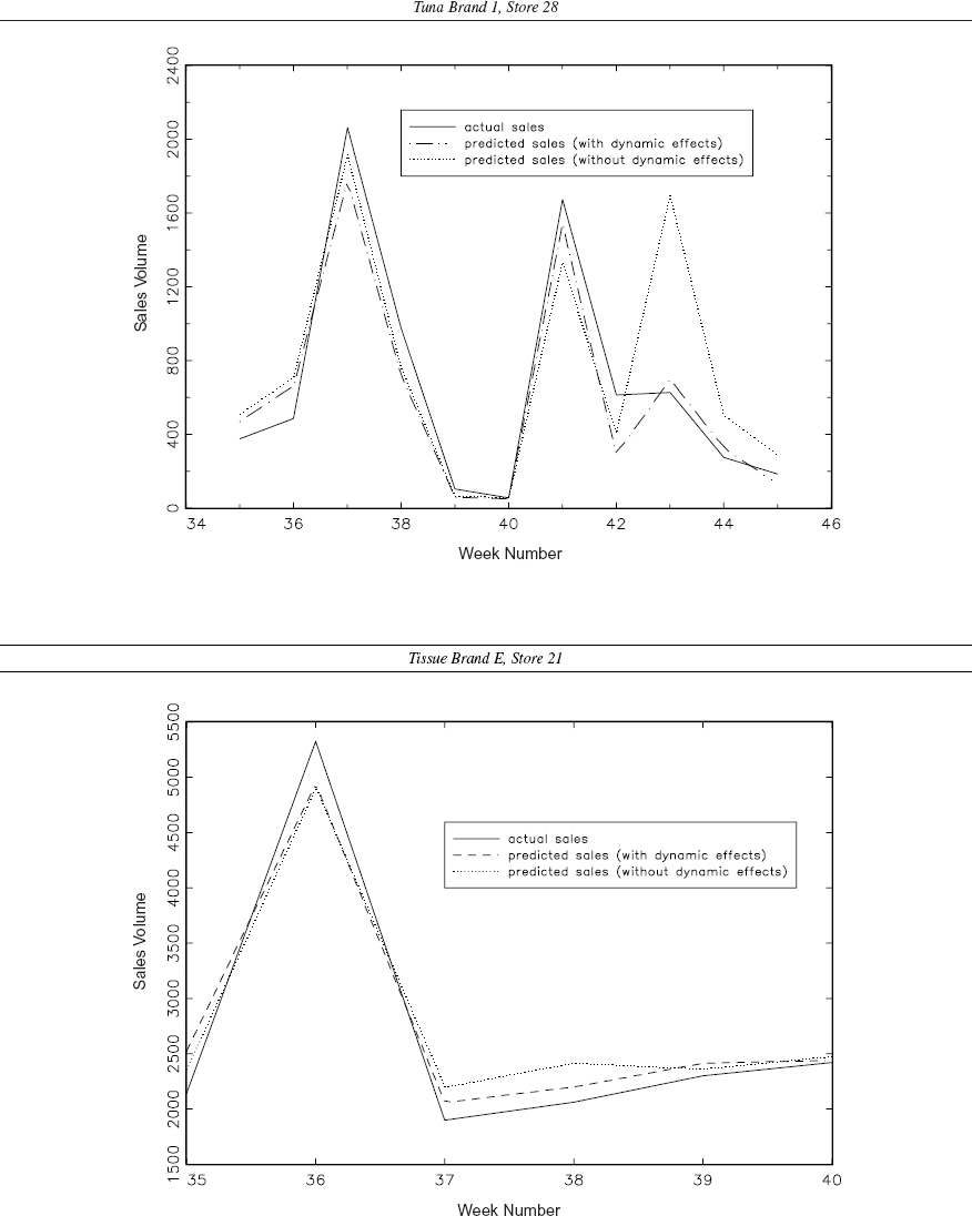
Actual Sales and Predicted Sales by (1) The Dynamic Effects Model and (2) The No Dynamic Effects Model

The second example is from tissue brand E sold in store 21. As is shown in the lower panel of Figure 2, the dynamic effects model approximates the postpromotion dip better than the no dynamic effects model (see weeks 37 and 38). Again, the no dynamic effects model was rejected (Table 2). This graph illustrates the subtleness of dynamic promotion effects and is more representative of brand sales graphs than the upper panel of Figure 2.

Conclusions

We investigated one of the mysteries of sales promotion research: the lack of postpromotion dips in store data. From studies of household panel data, it is known that consumers often accelerate their purchases in time and/or quantity because of promotions, which should result in a dip in purchases in the weeks following a promotion. This dip, however, is rarely observed in sales data. Extant arguments for the apparent lack of postpromotion dips imply that the dips may be difficult to detect by traditional models. Because brand sales are the aggregate of purchases across (heterogeneous) households, both pre- and postpromotion sales data may have complex patterns. Essentially, sales are shifted from multiple future and past periods into a current, promotion-based sales spike in a nontrivial way. Neslin and Schneider Stone (1996, p. 92) suggest that researchers “conduct sophisticated distributed lag analyses on weekly sales data in the hopes of measuring the postpromotion dip statistically.” Our modeling approach reflects the multitude of factors that pertain to dynamic promotion effects, and we obtain postpromotion dips convincingly.

We use an econometric model to regress brand-level sales on current, lagged, and lead price discount variables (price indices) for three different distributed lead and lag structures: an Almon model, an unrestricted dynamic effects model, and an exponential decay model. The unrestricted dynamic model is flexible but not parsimonious. The exponential decay model is the least flexible and the most parsimonious, and the Almon polynomial model is in between these extremes. More important, we distinguish the effects of four types of price discounts: without support, with feature-only support, with display-only support, and with feature and display support.

We applied the models to nine brands in two product categories: tuna fish and toilet tissue. Within each of these three models, we varied lead and lag lengths as well as the parameters describing the lag structure. For each brand, we selected the model specification that minimizes the AIC. We tested the assumption of parameter homogeneity among stores (no evidence of heterogeneity) and reestimated the models by accounting for nonzero autocorrelation or heteroscedasticity if necessary.

Our main findings across two product categories include the following:

•

Significant dynamic promotion effects exist (for eight of the nine brands).

•

The dynamic effects can be substantial. Negative dynamic effects are indicative of acceleration effects that vary between 4 and 25% of the current sales effect across the two categories and across different support activities for discounts. These numbers are consistent with the results from household-level studies, which have found the acceleration effect to vary between 6 and 51%.

•

The conclusion for researchers is that the postpromotion dip paradox does not need to exist: Household-level studies and this store-level study find acceleration effects of comparable sizes.

•

For managers, our results suggest that the results from models that accommodate only current sales effects from a promotion may be misleading. Managers should insist on obtaining the sum of the current and dynamic effects from a model that accounts for (1) purchase acceleration effects and (2) display extension effects.

•

Given the complexity of dynamic sales promotion effects, it is advisable to use a flexible specification, such as the unrestricted model or the Almon model. We find that the percent net gains (Table 3, Panel C) are similar for the Almon and unrestricted models, whereas the exponential decay model produces different results. Overall, the unrestricted model is the closest to the best model results. It is also the model that is easiest to implement.

An interesting future research issue in this context is the accommodation of within-store and between-store heterogeneity in models of store sales. Within-store heterogeneity can occur because of changes in the composition of the households that purchase items from the product category over time. The use of time-varying response parameters is one way to account for such effects. Between-store heterogeneity may result from customer, assortment, and other differences between stores. Even though we found no evidence in favor of this type of heterogeneity, it may be relevant for other categories. Hsiao, Appelbe, and Dineen (1993) provide a general framework for varying parameter panel data models.

From a substantive perspective, it will be useful to apply distributed lead and lagged models to other product categories to discover commonalities and idiosyncrasies. With results for a much larger number of items, it should be instructive to explore the effects of product category and brand measures, marketing activities (e.g., interpromotion periods, depth of price cuts), and consumer characteristics on the observed dynamics.

References

Bell

David R.

, Chiang

Jeongweng

, and Padmanabhan

(1999), “The Decomposition of Promotional Response: An Empirical Generalization,” Marketing Science, 18 (Winter), 504–26.

Blattberg

Robert C.

, Briesch

Richard

, and Fox

Edward J.

(1995), “How Promotions Work,” Marketing Science, 14 (Part 2 of 2), G122–32.

Blattberg

Robert C.

, and Neslin

Scott A.

(1990), Sales Promotion, Concepts, Methods and Strategies. Englewood Cliffs, NJ: Prentice Hall.

Blattberg

Robert C.

, and Wisniewski

Kenneth J.

(1989), “Price-Induced Patterns of Competition,” Marketing Science, 8 (Fall), 291–309.

Bucklin

Randolph E.

, and Gupta

Sunil

(1999), “Commercial Use of UPC Scanner Data: Industry and Academic Perspectives,” Marketing Science, 18 (Fall), 247–73.

Chiang

Jeongwen

(1991), “A Simultaneous Approach to the Whether, What and How Much to Buy Questions,” Marketing Science, 10 (Fall), 297–315.

Christen

Markus

, Gupta

Sachin

, Porter

John C.

, Staelin

Richard

, and Wittink

Dick R.

(1997), “Using Market-Level Data to Understand the Promotion Effects in a Nonlinear Model,” Journal of Marketing Research, 36 (August), 322–34.

Doyle

Peter

, and Saunders

John

(1985), “The Lead Effect of Marketing Decisions,” Journal of Marketing Research, 22 (February), 54–65.

Foekens

Eijte W.

, Leeflang

Peter S.H.

, and Wittink

Dick R.

(1994), “A Comparison and an Exploration of the Forecasting Accuracy of a Nonlinear Model at Different Levels of Aggregation,” International Journal of Forecasting, 10 (2), 245–61.

10.

Foekens

Eijte W.

, Leeflang

Peter S.H.

, and Wittink

Dick R.

(1999), “Varying Parameter Models to Accommodate Dynamic Promotion Effects,” Journal of Econometrics, 89 (1), 249–68.

11.

Grover

Rajiv

, and Srinivasan

(1992), “Evaluating the Multiple Effects of Retail Promotions on Brand Loyal and Brand Switching Segments,” Journal of Marketing Research, 29 (February), 76–89.

12.

Gupta

Sachin

, Chintagunta

Pradeep K.

, Kaul

Anil

, and Wittink

Dick R.

(1996), “Do Household Scanner Data Provide Representative Inferences from Brand Choices? A Comparison with Store Data,” Journal of Marketing Research, 33 (November), 383–98.

13.

Gupta

Sunil

(1988), “Impact of Sales Promotion on When, What, and How Much to Buy,” Journal of Marketing Research, 25 (November), 342–55.

14.

Hsiao

Cheng

, Appelbe

Trent W.

, and Dineen

Christopher

(1993), “A General Framework for Panel Data Models with an Application to Canadian Customer-Dialed Long Distance Telephone Service,” Journal of Econometrics, 59 (1), 63–86.

15.

Inman

Jeffrey

, McAlister

Leigh

, and Hoyer

Wayne D.

(1990), “Promotion Signal: Proxy for Price Cut?” Journal of Consumer Research, 17 (June), 74–81.

16.

Judge

George G.

, Griffiths

W.E.

, Hill

R. Carter

, Lütkepohl

Helmut

, and Lee

Tsoung-Chao

(1985), The Theory and Practice of Econometrics, 2d ed. Singapore: John Wiley & Sons.

17.

Kalwani

Manohar U.

, Yim

Chi Kin

, Rinne

Heikke J.

, and Sugita

Yoshi

(1990), “A Price Expectation Model of Customer Brand Choice,” Journal of Marketing Research, 27 (August), 251–62.

18.

Kmenta

Jan

(1986), Elements of Econometrics. New York: Macmillan Publishing Company.

19.

Körösi

Gábor

, Mátyás

László

, and Székely

István P.

(1992), Practical Econometrics. Aldershot, England: Avebury.

20.

Kumar

, and Leone

Robert P.

(1988), “Measuring the Effect of Retail Store Promotion on Brand and Store Substitution,” Journal of Marketing Research, 25 (May), 178–85.

21.

Lattin

James M.

, and Bucklin

Randolph E.

(1989), “Reference Effects of Price and Promotion on Brand Choice Behavior,” Journal of Marketing Research, 26 (August), 299–310.

22.

Leone

Robert P.

(1987), “Forecasting the Effect of an Environmental Change on Market Performance: An Intervention Time Series Approach,” International Journal of Forecasting, 3 (4), 463–78.

23.

Litvack

David S.

, Calantone

Roger J.

, and Warshaw

Paul R.

(1985), “An Examination of Short-Term Retail Grocery Price Effects,” Journal of Retailing, 61 (Fall), 9–26.

24.

Moriarty

Mark M.

(1985), “Retail Promotional Effects on Intraand Interbrand Sales Performance,” Journal of Retailing, 61 (Fall), 27–47.

25.

Narasimhan

Chakravarthi

, Neslin

Scott A.

, and Sen

Subrata K.

(1996), “Promotional Elasticities and Category Characteristics,” Journal of Marketing, 60 (April), 17–30.

26.

Neslin

Scott A.

, and Stone

Linda G. Schneider

(1996), “Consumer Inventory Sensitivity and the Postpromotion Dip,” Marketing Letters, 7 (1), 77–94.

27.

Papatla

Purushottam

, and Krishnamurthi

Lakshman

(1996), “Measuring the Dynamic Effects of Promotions on Brand Choice,” Journal of Marketing Research, 33 (February), 20–35.

28.

Rust

Roland T.

, Simester

Duncan

, Brodie

Roderick J.

, and Nilikant

(1995), “Model Selection Criteria: An Investigation of Relative Accuracy, Posterior Probabilities, and Combinations of Criteria,” Management Science, 41 (February), 322–33.

29.

Stewart

Jon

(1991), Econometrics. Hemel Hemstead, England: Philip Allan.

30.

Winer

Russell S.

(1986), “A Reference Price Model of Brand Choice for Frequently Purchased Products,” Journal of Consumer Research, 13 (September), 250–56.

31.

Wittink

Dick R.

, Addona

Michael J.

, Hawkes

William J.

, and Porter

John C.

(1988), “The Estimation, Validation, and Use of Promotional Effects Based on Scanner Data,” working paper, Johnson Graduate School of Management, Cornell University.