Designing Conjoint Choice Experiments Using Managers' Prior Beliefs

Abstract

The authors provide more efficient designs for conjoint choice experiments based on prior information elicited from managers about the parameters and their associated uncertainty. The authors use a Bayesian design procedure that assumes a prior distribution of likely parameter values and optimizes the design over that distribution. The authors propose a way to elicit prior information from managers and show in Monte Carlo studies that the procedure provides more efficient designs than the current procedures. The authors provide an empirical application, in which they elicit prior information on the parameter values and the associated uncertainty from managers. Here, the Bayesian design provides 30%-50% lower standard errors of the estimates and an expected predictive validity that is approximately 20% higher.

A conjoint choice design should provide as much information as possible on the parameters of the choice model calibrated on the collected data. Several authors have addressed the problem of how to construct designs with higher efficiency (Bunch, Louviere, and Anderson 1994; Huber and Zwerina 1996; Kuhfeld, Tobias, and Garratt 1994; Lazari and Anderson 1994) and provide methods to produce those designs. Constructing designs with improved efficiency has become more and more important because problems of lengthy questionnaires are increasingly troubling market researchers. The dilemma is the trade-off between the increasing quantity of information obtained at higher costs and the decreasing quality of that information because of such effects as respondent fatigue and boredom.

More efficient designs enable a reduction in the number of questions asked from a respondent as well as a reduction in the number of respondents. We are interested in generating designs for conjoint choice experiments. Complications in the construction of these designs arise from the analysis of the data from conjoint choice experiments with the multinomial logit model (MNL; Louviere and Woodworth 1983). Contrary to experimental design methods for linear regression (Atkinson and Donev 1992; Lenk et al. 1996; Pilz 1991), for the MNL the construction of an efficient experimental design requires knowledge of the values of the parameters. This is so because the information on the parameters provided by the design is dependent on the value of those parameters. Unfortunately, the parameter values are unknown at the time the design is constructed, and researchers need to assume values to enable a design to be generated. Often, researchers construct designs by assuming that the parameters are zero. This construction can be motivated by the argument that the design achieves optimality under the null hypothesis of no effect of the attribute level in question. However, in many applications, zero parameter values are judged unlikely a priori by product or marketing managers, and the constructed design can have low efficiency at the parameter values that seem relevant from a management point of view. It is therefore desirable to optimize the design over nonzero parameter values, reflecting the managers' beliefs. However, in doing so, researchers must accommodate the uncertainty about those beliefs. This is what we set out to do in this article.

Huber and Zwerina (1996) provide a first and important effort to construct designs with improved efficiency when the parameters are assumed to be nonzero. They argue that in practice, conjoint questionnaires are often pretested on small samples, the results of which may provide reasonable priors for the construction of the design. However, this approach has limitations. First, some design should already be available for the pretest, and second, it is not known how efficient the constructed designs are if the true parameter values differ from the ones assumed in the pilot, because uncertainty about them is discarded. Researchers must obtain designs that take the uncertainty about the assumed parameter values into account. Such designs are expected to yield a higher efficiency across a wide range of parameter values. Uncertainty about specific values may be accommodated through a prior distribution over a range of plausible values. In this article, we address this issue and develop designs with improved efficiency that are constructed in a Bayesian fashion (for an excellent review of Bayesian experimental designs, see Chaloner and Verdinelli 1995), incorporating prior parameter distributions elicited from managers. We build on previous work in this area (Huber and Zwerina 1996), in that our designs pertain to a typical conjoint choice experimental setup for MNL models with qualitative predictors and main effects only.

In the next section, we describe the construction of Bayesian designs. First, we introduce the MNL model for choice experiments, and then we describe in more detail the design optimality criteria we use. We elaborate on the elicitation and use of prior distributions for the parameter values and propose a Bayesian approach to the construction of experimental designs. Then we compare the performance of a design obtained by Huber and Zwerina (1996) with Bayesian designs. In addition, we investigate the performance of our modified design-generating algorithm. We conduct Monte Carlo studies to investigate the relative efficiency of the designs under various conditions. In the following section, we provide an empirical application, in which we elicit prior information from management to yield improved choice designs. In the last section, we discuss limitations and extensions.

Choice Designs

In developing choice designs for the MNL model, we specify the utility of a subject for profile j in choice set s as

u_{js} = x'_{js} β + ε_{js},

(1)

where x_js is a k-vector of the attributes of the alternative j, β is a k-vector parameter weighting these attributes, and ε_js is an error term following an i.i.d. extreme value distribution. If the respondents are assumed to choose the profile with the highest utility of the J alternatives in choice set s, the probability that j is chosen can be expressed in closed form:

p_{js} = \frac{\exp (x_{js}^{'} β)}{\sum_{r = 1}^{J} \exp (x_{rs}^{'} β)} .

(2)

We assume a design in which all respondents are to be given the same choice sets. Because of the assumption of independence of the error terms, the choices made among the alternatives in different choice sets are independent. Then, the log-likelihood function is the sum of the log-likelihood functions of the choice sets; that is,

L = N \times \sum_{s = 1}^{S} \sum_{j = 1}^{J} f_{js} \times {ln p}_{js},

(3)

where f_js denotes the observed number of purchases of product j in choice set s divided by the total number of purchases, N. The information matrix, obtained as the variance of the first-order derivatives of the log-likelihood with respect to the parameters, is the sum of the choice-set–specific information matrices:

I (β) = N \times \sum_{s = 1}^{S} X_{s}^{'} (P_{s} - p_{s} p_{s}^{'}) X_{s},

(4)

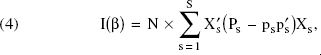
where X_s = [x_1s,…,x_Js]′, p_s = [p_1s,…,p_Js]′, and P_s = diag(p_1s, …, p_Js).

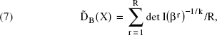
Our concern is to find a design of the product profiles that, given a number of choice sets, a number of alternatives in the choice sets, and a number of attribute levels, has improved efficiency. Following the other design-generation procedures provided in the literature, we consider the size of the choice set to be fixed by the researcher before design construction. We accept minimal attribute-level overlap as a constraint on the design, which means that within a choice set, the same attribute level should occur as few times as possible. Huber and Zwerina (1996) use level balance as a design constraint, which implies that all levels of an attribute occur in the same frequencies. However, we show subsequently that sacrificing strict level balance enables us to generate more efficient designs than enforcing this criterion does. It appears that the design-optimization procedure we use yields designs that are approximately level balanced, even without explicitly enforcing this constraint. Huber and Zwerina (1996) also use orthogonality as a design optimality constraint, because according to their definition, together with minimal level overlap and level balance, it yields efficient designs. In their definition, a design is orthogonal if X'X is diagonal for a suitably coded × (see also Kuhfeld, Tobias, and Garratt 1994). This design orthogonality (Lindsey 1996, p. 235) is of limited use, because in the MNL model it does not imply that the parameters themselves are independent (though design orthogonality tends to reduce the strength of the relationships among parameters). A more useful concept is information orthogonality (Lindsey 1996, p. 236), in which the parameter estimates are truly independent. However, from Equation 4 it appears that if the parameters deviate from zero, finding any design that satisfies information orthogonality is unlikely. Therefore, orthogonality and level balance will not play a role in our procedure to develop efficient choice designs. We look for designs that maximize the information on the estimates as represented in the Fisher information matrix in Equation 4 under the constraint of minimal level overlap. A widely accepted one-dimensional measure of information is the determinant of the information matrix (Huber and Zwerina 1996; Kuhfeld, Tobias, and Garratt 1994). It is motivated from the confidence ellipsoid for β that equals

{β: {(β - \hat{β})}^{'} I (\hat{β}) (β - \hat{β}) \leq constant},

(5)

where $\hat{β}$ is the ML estimate of β and has a volume proportional to ${[det I (\hat{β})]}^{- 1 / 2}$ (Silvey 1980). Researchers usually employ the D_P-error: D_P-error = det[I(β)]^−1/k as a one-dimensional measure of the efficiency of a design. Here, k is the dimensionality of the parameter vector, and the exponent serves to “adjust” the information for the dimensionality of the parameter vector. The power 1/k normalizes the determinant of the information matrix, making it proportional to the number of respondents.

It should be noted that we cannot prove that the designs we generate are strictly optimal, nor are they expected to be. There are several reasons for this. First, by enforcing minimal level overlap, we optimize the choice design under a constraint that may make it less efficient. We search for “optimal” designs within the class of minimal level overlap designs. Second, we optimize a scalar measure of the information, det[I(β)]^−1/k, because this measure has intuitive appeal and has been used previously in the design of conjoint choice experiments (Huber and Zwerina 1996) and other experiments for logit models (Zacks 1977). However, other measures are possible, for example, ln{det[I(β)]}. This measure is appealing from a Bayesian perspective because it can be derived from a utility function of a design based on Shannon information (Chaloner and Verdinelli 1995). Design optimality is only defined with respect to the particular scalar measure of information we use, but our approach can easily be extended to include others, for example, the ln{det[I(β)]} criterion. Third, we use heuristic search procedures to find the optimum. Although those heuristics yield designs with improved efficiency, they may not yield optimal efficiency. Therefore rather than refer to “optimal” designs, we refer to designs with “improved efficiency” or “more efficient” designs. Table 1 provides an overview of the criteria considered by previous authors.

Table 1

PREVIOUS RESEARCH ON EFFICIENT DESIGNS IN MARKETING

Authors	Year	Criterion	Assumed Parameters	Algorithm^a
Kuhfeld, Tobias, and Garrat	1994	det(X'X)	—	Modified Federov
Lazari and Anderson	1994	det(X'X)	—	Not specified
Huber and Zwerina	1996	det[I(β)⁻¹]	β₀	R, S
This article	2001	det[I(β)⁻¹]	f(β₀, σ₀)	R, S, C

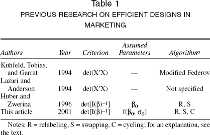
Notes: R = relabeling, S = swapping, C = cycling; for an explanation, see the text.

Eliciting and Using Prior Information

We propose to elicit prior information on the parameters from product or marketing managers in the company that issues the study and to use that in design construction. Managers hold prior beliefs on the share of consumers that will purchase a product with a specific attribute level. Such prior beliefs are commonly used in selecting the attributes and levels to be included in a design, but though a priori beliefs could explicitly be allowed to affect the design itself, to date they have not been used in that way.

How can prior information on choice model parameters be elicited from managers? Subjective Bayesian theory states that personal beliefs can be reflected through subjective probability statements (Berger 1985, p. 75): It assumes that people can conceive of uncertainty about events as probabilities and can coherently express those probabilities (Savage 1976). We wish to elicit prior beliefs from managers in the form of a (95%) credible set that involves the upper and lower bounds of the prior probability distribution of model parameters (Shafer 1982). However, instead of eliciting beliefs for a parameter β₁ directly, we propose to elicit managers' beliefs about the relative f₁ (market shares) with which customers in the population will choose a product with attribute level l. We then derive the corresponding subjective probability distribution (SPD) of the parameter from it by a transformation. The motivation for doing so is that prior distributions are not invariant under transformations. Therefore, equivalent prior distributions for parameters in differently parameterized choice models may lead to different prior distributions for the choice frequencies. Techniques for elicitation of beliefs on relative frequencies are well developed in the psychological literature, but it may be difficult for managers to state beliefs on relatively abstract constructs as parameters.

Various elicitation techniques have been proposed (see Van Lenthe 1993), which attempt to control the reliability and validity of the stated beliefs (Lichtenstein, Fischhoff, and Phillips 1982). In particular, overconfidence (Yates et al. 1989) has been reported to be a major problem. Scoring rules are used to give feedback on individual assessments in an attempt to alleviate overconfidence. With strictly proper scoring rules, individual assessors are stimulated to report only true beliefs, because they can maximize the score only if the stated SPD corresponds to their subjective knowledge.

We use a paper-and-pencil version of the elicitation method proposed by Van Lenthe (1993), employing proper scoring rules in a graphically oriented elicitation task. Managers are asked to provide a direct visualization of their SPD of customer choice by drawing it, for each attribute in the design, in panels as is shown in Figure 1. Feedback is provided in terms of upper and lower bounds for the subjective judgments, and multiple tries are allowed. In the task, we ask the managers to think of these probabilities as if the products formed by all possible combinations of the attributes and levels are available to consumers and invite the managers to assess the choice probabilities for a product that we present with specific levels of one particular attribute. 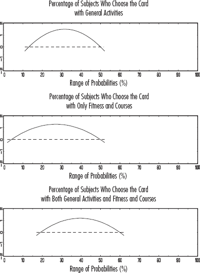Van Lenthe (1993) extensively investigates the performance of his method, which provides estimates of the lower π_l, and upper ${\bar{π}}_{l}$ bounds of the subjective probability distribution function of choice frequencies.

Figure 1

EXAMPLE OF SUBJECTIVE PROBABILITIES ASSESSED BY A MANAGER

Despite the scoring rule used, the manager, specifying an interval for the choice frequencies, may still display over-confidence. Following Almond (1996, p. 241), we therefore take the managers' judgment to hold with a probability of 95%, which is equivalent to eliciting a 95% credibility interval from them, and fit a normal distribution to the 95% credible interval. From the elicited prior distribution of the frequencies, we derive the prior distribution of the parameters, which has a density denoted $\hat{f} (β_{1})$ , by employing an inverse logit transformation as shown in Equations 8 and 9 in the following application.

Constructing the Design

Adopting a Bayesian approach to design construction (see Atkinson and Donev 1992, p. 211; Chaloner and Verdinelli 1995), we use the prior distribution of the logit coefficients $\hat{f} (β)$ thus obtained to reflect subjective beliefs in the probabilities that particular parameter values occur. The optimal design is the one that minimizes the D_B-error, that is, the expectation of the D_P-error over the prior distribution of the parameter values:

D_{B} -error = E_{β} [\det I {(β)}^{- 1 / k}] = \int_{ℝ^{k}} \det I {(β)}^{- 1 / k} \hat{f} (β) dβ .

(6)

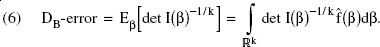
We note that this criterion is necessarily approximate, as it is based on an asymptotic approximation to the posterior distribution. The expected information is approximated by drawing R times from $\hat{f} (β)$ , and computing

{\tilde{D}}_{B} (X) = \sum_{r = 1}^{R} \det I {(β^{r})}^{- 1 / k} /R,

(7)

where β^r is a draw from $\hat{f} (β)$ . We use R = 1000.¹ Then we evaluate this approximate value for designs constrained to have minimal level overlap and submit it to the algorithms for finding the optimum value over the design space. We take the expectation of the design criterion over the prior distribution of the parameters so that prior uncertainty translates into a spread of the design points. This approach is appropriate, because in the absence of data, the prior and the posterior distributions coincide: The prior is also called the preposterior in this context. Note that in this formulation we ignore the prior variance, say S_β. An alternative criterion is ${\int_{ℝ^{k}} det [I (β) + S_{β}]}^{- 1 / k} \hat{f} (β) d β$ . However, Chaloner and Verdinelli (1995) argue in favor of the criterion we use, because it allows different prior information to be used in the design and analysis and is appealing when a non-Bayesian framework is adopted for analysis. In addition, our criterion is based on an asymptotic approximation to the posterior, and the prior vanishes in that case. Our design criterion has been shown to have good properties (Atkinson and Donev 1992, pp. 214, 218).

We investigated the effect of the number of draws used on the efficiency of the generated designs: The difference in the number of subjects needed to achieve the same efficiency compared with a design based on 10,000 draws was 2% or less.

The optimization problem can be formally represented as

\min_{X} {\tilde{D}}_{B} (X),

subject to X having minimal level overlap, given $\hat{f} (β)$ , the prior distribution of β. The tools we use for determining the design that provides the largest information and satisfies minimal level overlap are relabeling and swapping, as developed by Huber and Zwerina (1996). In addition, we propose the use of a procedure we call cycling. We conjecture that cycling may improve on Huber and Zwerina's (1996) algorithm. The reason that such heuristic procedures are used is that an exhaustive search over the entire design space is not feasible, except for small designs.² The three stages of our algorithm—relabeling, swapping, and cycling—operate as stated in the next section.³

For a class of small designs (i.e., 3²/2/6), we experimented with a search over all possible designs with minimal level overlap, which is possible though time consuming. It appeared that the distribution of the D_P-error criterion is highly skewed and extremely peaked. Nevertheless, the heuristic search algorithms did a good job and recovered the optimum in 46% of the cases in 1000 runs, and in the remaining 54% it was within 3% of the optimum. There is no guarantee that this is also the case for larger designs, in which for an exhaustive search an impractical number of evaluations of the D-errors must be made. For example, in the case of the 3⁴/2/15 designs, the total number of designs with minimal level overlap is approximately 10³⁰.

Gauss codes for these algorithms are available from the authors.

Design-Generating Algorithms

Relabeling permutes the levels of the attributes across choice sets. Take the first attribute and its levels across all choice sets. Take one particular permutation of the levels; for example, for three levels, this may be 2 3 1, one of the six possible permutations. Then reassign the levels of the attribute according to this permutation; that is, replace Level 1 by 2, 2 by 3, and 3 by 1. Do the same for other attributes for one particular permutation of their levels. Then go back to Attribute 1 and try a different permutation of its levels, as well as for the other attributes. Thus, the relabeling algorithm searches for a combination of permutations for which the corresponding design has the smallest error (either D_P-or D_B-error). (This is the same as in Huber and Zwerina's [1996] algorithm.)

Swapping involves switching two attribute levels among alternatives within a choice set. Assume two alternatives. The algorithm starts with the first choice set, takes the level of the first attribute, and swaps it with the level of that attribute in the second alternative. Then it does the same with the second attribute, and so on until the last attribute. Also consider simultaneous swaps for several attributes subsequently. Then, the algorithm proceeds to the second choice set and passes through all choice sets. If an improvement in information occurs, the procedure returns to the first choice set and proceeds until no improvement is possible. (Our algorithm is slightly different from that used by Huber and Zwerina [1996].)

Cycling is a combination of cyclically rotating the levels of an attribute and swapping them. The algorithm starts with the first attribute in the first choice set. It cyclically rotates the levels of the attribute until all possibilities are exhausted. Thus, if there are three levels, replace Level 1 with Level 2, Level 2 with 3, and Level 3 with 1. Continue this until the original configuration is obtained again. Then apply a swap and cycle again until all possibilities are exhausted. Continue in this manner by alternating swapping and cycling until all possibilities are verified. Then go on to the second choice set and so on until the last choice set. Then move to the second attribute and pass through all attributes proceeding in the same way as with the first attribute. At each stage, if an improvement is made, the procedure starts over from the first attribute in the first choice set. When no improvement is possible, the procedure stops.

Comparisons and Monte Carlo Studies

Comparison with Huber and Zwerina (1996)

In this section, we compare Bayesian designs with the designs provided by Huber and Zwerina (1996; henceforth HZ). In addition, we investigate the incremental contribution of the cycling algorithm over the relabeling and swapping algorithm. Consider the design from HZ of type 3⁴/2/15; that is, there are 15 choice sets, there are two alternatives in each set with four attributes, and each attribute has three levels: 1, 2, and 3. We use effect coding that assigns [1 0], [0 1], and [-1 −1] to the levels 1, 2, and 3, respectively. Assume the coefficients to be fixed at p₀ = [-1 0 −1 0 −1 0 −1 0]′, the values used by HZ. As HZ explain, this set of coefficients produces choice probabilities that are the same when, instead of coding, numerical values are assigned to the attribute levels and the coefficients are all equal to one.

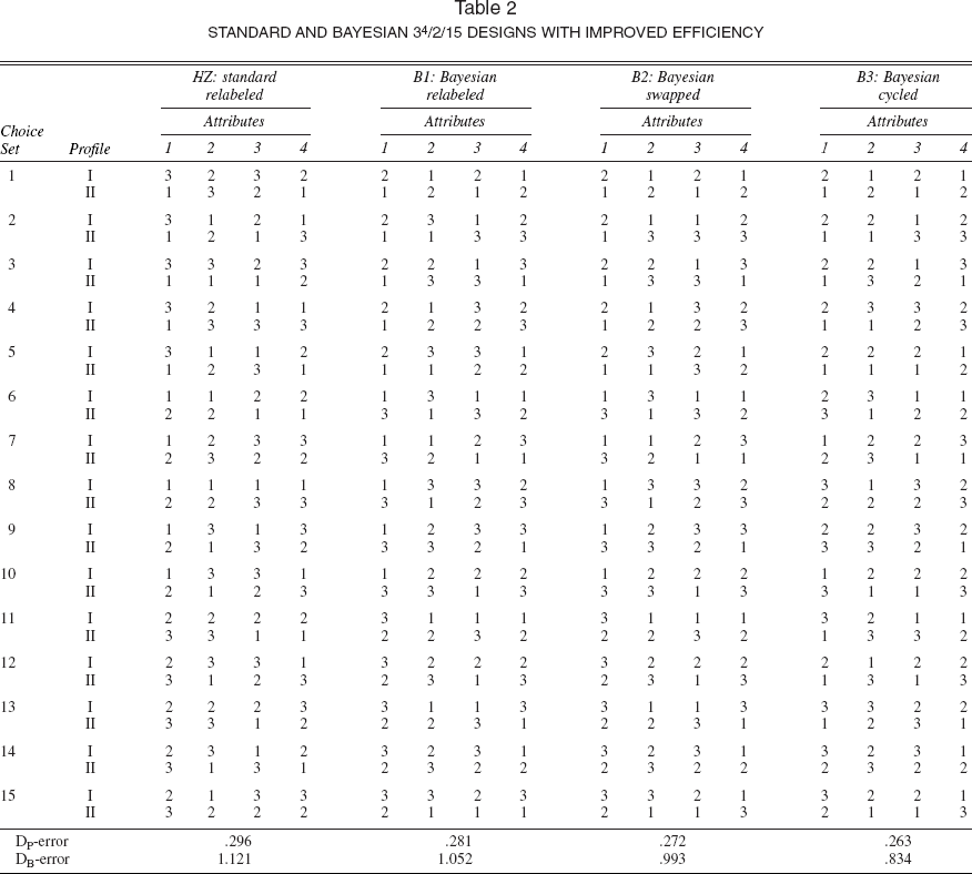
The leftmost column of Table 2 presents the design determined by HZ (HZ, Table 3, p. 313) from relabeling a starting design. Note that we use the relabeled design and not the swapped design (which was reported by HZ to provide a lower D_P-error). The reason is that HZ only provide the complete design generated by relabeling, and we believe that it provides a useful benchmark. (Subsequently, we present a Monte Carlo study in which we use the standard design obtained through relabeling, swapping, and cycling as a baseline.) In the bottom row of Table 2, the D_P- and D_B-errors are presented, which reflect the efficiencies of the designs. Table 2 also presents the improved Bayesian relabeled, swapped, and cycled designs, denoted B1, B2, and B3, respectively. Because prior management information is lacking, for these Bayesian designs we take the parameters of the prior distribution as follows: We fix the mean at β₀ provided by HZ and take the square root of the covariance matrix Σ₀^½ equal to the identity matrix. The designs B1, B2, and B3 are obtained by minimizing the D_B-error (see Equation 6), where β ∼ N(β₀, Σ₀). Note that this procedure reveals the improvement obtained only by accommodating parameter uncertainty through a prior distribution, because the mean parameter values are the same for the standard and Bayesian procedures. We believe that neglecting that uncertainty is logically inconsistent, because if the parameters were precisely known, no design needs to be generated.

Table 2

STANDARD AND BAYESIAN 3⁴/2/15 DESIGNS WITH IMPROVED EFFICIENCY

		HZ: standard relabeled				B1: Bayesian relabeled				B2: Bayesian swapped				B3: Bayesian cycled
		Attributes				Attributes				Attributes				Attributes
Choice Set	Profile	1	2	3	4	1	2	3	4	1	2	3	4	1	2	3	4
1	I	3	2	3	2	2	1	2	1	2	1	2	1	2	1	2	1
	II	1	3	2	1	1	2	1	2	1	2	1	2	1	2	1	2
2	I	3	1	2	1	2	3	1	2	2	1	1	2	2	2	1	2
	II	1	2	1	3	1	1	3	3	1	3	3	3	1	1	3	3
3	I	3	3	2	3	2	2	1	3	2	2	1	3	2	2	1	3
	II	1	1	1	2	1	3	3	1	1	3	3	1	1	3	2	1
4	I	3	2	1	1	2	1	3	2	2	1	3	2	2	3	3	2
	II	1	3	3	3	1	2	2	3	1	2	2	3	1	1	2	3
5	I	3	1	1	2	2	3	3	1	2	3	2	1	2	2	2	1
	II	1	2	3	1	1	1	2	2	1	1	3	2	1	1	1	2
6	I	1	1	2	2	1	3	1	1	1	3	1	1	2	3	1	1
	II	2	2	1	1	3	1	3	2	3	1	3	2	3	1	2	2
7	I	1	2	3	3	1	1	2	3	1	1	2	3	1	2	2	3
	II	2	3	2	2	3	2	1	1	3	2	1	1	2	3	1	1
8	I	1	1	1	1	1	3	3	2	1	3	3	2	3	1	3	2
	II	2	2	3	3	3	1	2	3	3	1	2	3	2	2	2	3
9	I	1	3	1	3	1	2	3	3	1	2	3	3	2	2	3	2
	II	2	1	3	2	3	3	2	1	3	3	2	1	3	3	2	1
10	I	1	3	3	1	1	2	2	2	1	2	2	2	1	2	2	2
	II	2	1	2	3	3	3	1	3	3	3	1	3	3	1	1	3
11	I	2	2	2	2	3	1	1	1	3	1	1	1	3	2	1	1
	II	3	3	1	1	2	2	3	2	2	2	3	2	1	3	3	2
12	I	2	3	3	1	3	2	2	2	3	2	2	2	2	1	2	2
	II	3	1	2	3	2	3	1	3	2	3	1	3	1	3	1	3
13	I	2	2	2	3	3	1	1	3	3	1	1	3	3	3	2	2
	II	3	3	1	2	2	2	3	1	2	2	3	1	1	2	3	1
14	I	2	3	1	2	3	2	3	1	3	2	3	1	3	2	3	1
	II	3	1	3	1	2	3	2	2	2	3	2	2	2	3	2	2
15	I	2	1	3	3	3	3	2	3	3	3	2	1	3	2	2	1
	II	3	2	2	2	2	1	1	1	2	1	1	3	2	1	1	3
D_P-error		.296				.281				.272				.263
D_B-error		1.121				1.052				.993				.834

Table 3

ATTRIBUTES AND LEVELS OF THE SPORTS CLUB MEMBERSHIP APPLICATION

	Attributes
Levels	Location	Period	Activities	Clubs	Price
1	A	1 trimester	General	No clubs	40
2	B	2 trimesters	Fitness + courses	Student clubs	75
3	Both	3 trimesters	All	20% discount	125

Visual inspection of the designs in Table 2 shows that all designs are reasonable in terms of composition of profiles and choice sets. The Bayesian design produces the lowest D_B-error, which is expected because that is the criterion minimized by it. But it also produces a lower D_P-error, which makes it preferable over HZ's relabeled design. Note that all DP- and D_B-errors are substantially lower for the Bayesian designs produced by cycling than for the designs produced by relabeling and by relabeling and swapping.⁴ This illustrates the superior performance of the proposed cycling algorithm.

In general, cycling improves over swapping for designs in which the number of alternatives in a choice set is not equal to the number of attribute levels.

Monte Carlo Studies

In the previous comparison, the D_P- design errors were computed at the specific parameter values assumed in constructing the respective designs. It is our contention that the Bayesian approach yields more efficient designs over a wide range of the parameter space. To investigate this, we conduct a Monte Carlo study that compares, in terms of the D_P-error, the performance of the standard HZ-type design with the Bayesian design. We construct the standard design with four attributes and three levels, analogous to HZ, in that we use relabeling, swapping, and cycling in its construction. Thus, the comparison of the Bayesian design with the standard design is unconfounded by the optimization procedure. All designs are based on 15 choice sets with 2 alternatives. In the Monte Carlo study, we investigate the sensitivity of the Bayesian design to the specified prior distribution as follows: For both the standard and the Bayesian designs, we choose β₀ as defined in the previous section. But because the performance of the Bayesian design may be sensitive to the choice of Σ₀ in the prior distribution, we vary that parameter in the Monte Carlo study. In particular, we construct six Bayesian designs, using Σ₀ = σ²₀I_k with six different values: σ₀ = .10, .25, .50, .75, 1.00, and 2.00. We draw 1000 true parameter vectors from the normal distribution, for each of 36 grid points, with a mean β₀ and a standard deviation varying between 0 and 5 on the grid. At each of the 36,000 draws, we evaluate the D_P-errors of the standard and the six Bayesian designs.

To assess the relative performance of the Bayesian designs, we compute the increase in the number of respondents needed for the standard design to have the same D_P-efficiency as the Bayesian design. This measure, if positive, reflects by what percentage we can reduce the number of respondents using a Bayesian design in order to obtain estimates that are as efficient as those from the standard design. (If it is negative, it shows by what percentage we should reduce the number of respondents for the standard design in order to obtain the same efficiency as with the Bayesian design.) Note that we again compare the designs on the criterion that is most favorable to the standard HZ design, because that is the design that maximizes the D_P-efficiency.

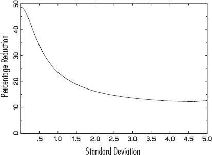
Figure 2 shows the extent to which the Bayesian design is more efficient. The standard deviations of the true parameters, reflecting their variation around the ones assumed in design construction, are shown on the x-axis, and the difference in the numbers of subjects needed for the Bayesian design relative to the standard design is on the y-axis. The different panels show the results obtained for different values of σ₀. Figure 2 shows that if the prior distribution assumed in the Bayesian design reflects little uncertainty (i.e., σ₀ = .1), the two designs need about the same number of subjects. This is to be expected, because it corresponds to a situation in which the parameter values are almost exactly known. (For σ₀ = .05, the Bayesian and the standard designs are exactly the same.) If the prior distribution assumed for the parameters reflects more uncertainty (i.e., for σ₀ = .25 and .5), a reduction of approximately 10% in the number of subjects is obtained in most cases. Each of the panels shows that if the true parameters are very close to the assumed ones in generating the designs (left-hand side of the graphs), the standard design tends to do better. This seems intuitive: If the researcher knows the values of the coefficients with a high degree of certainty, then there is not much use in employing a Bayesian design construction method. These results reveal that overconfidence of managers in eliciting their prior beliefs may affect the constructed design seriously. For larger values of σ₀, such as .75, 1.0, and 2.0, a substantial reduction of 15–22 is obtained. In our study, we provide only a lower bound for the relative performance of the Bayesian designs for three reasons. First, the Monte Carlo study reflects only the effect of including prior uncertainty on the parameter values, because the mean parameter values are the same for the standard and the Bayesian design. In practice, as we show subsequently, the Bayesian design may be appreciably better because it is based on different mean parameter values derived from managers' beliefs. Second, we note that the true parameter values were generated from draws from normal distributions centered around the assumed parameter values, but with different standard deviations, as shown on the x-axis of the graphs. Even if the standard error is large, a substantial proportion of the true parameters will be generated close to the assumed ones because of the symmetric unimodal shape of the normal distribution, which thus provides relative advantage to the standard design. Third and finally, we evaluate the relative improvement of the Bayesian design in terms of the D_P- rather than the D_B-error, which is to the advantage of the standard design.

Figure 2

PERCENTAGE REDUCTION OF SUBJECTS NEEDED FOR THE BAYESIAN DESIGN COMPARED WITH THE STANDARD DESIGN WITH THE SAME EFFICIENCY

In the Monte Carlo study described previously, the design involves four attributes and three levels. How will the design-generating procedures perform for different numbers of attributes and levels? To answer that question, we conduct another Monte Carlo Study. On the basis of either three or five attributes and three or four levels of the attributes, we construct four possible design conditions. (All designs are based on 24 choice sets with 2 alternatives.) For both the standard and the Bayesian designs, we choose β₀ as defined previously and use three different values: σ₀ = .20, 1.00, and 2.00. Thus, we evaluate the performance of the Bayesian compared with the standard design under 12 conditions. For each of those conditions, we draw 1000 true parameter vectors from the normal distribution for each of 36 grid points (36,000 draws in total), all with a mean β₀ and a standard deviation varying on the grid between 0 and 5, as in the previous study. At each draw, we evaluate the D_P-errors of the standard and the Bayesian designs and compute the increase in the number of respondents needed for the standard design to have the same D_P-efficiency as the Bayesian design. Note again that the criterion for comparison is itself most favorable to the standard design.

Figure 3 shows the results and reveals several interesting issues. First, it shows that when taking a small value of σ₀ (i.e., .20), the Bayesian design provides only a minor improvement over the standard design, irrespective of the design condition. The reason is the very limited prior uncertainty on the parameters, which makes the designs converge. Second, the effect of the number of attributes is limited. It does seem, however, that for a larger number of attributes, the difference in performance of the Bayesian and the standard design is less than the difference for a smaller number of attributes. The effect of the number of levels is even more interesting: If the attributes in the design are defined at a larger number of levels, the improvement of the Bayesian design over the standard design is larger. This holds in particular for the case in which the number of attributes is larger. Here, we see improvements that may range up to 30%–40%. A preliminary conclusion that emerges from this study is that in particular, for more complex designs (i.e., the ones with larger numbers of attributes and levels), the improvements of using a Bayesian design procedure may be substantial. These results will need to be corroborated in larger Monte Carlo studies that employ a wider range of numbers of choice sets, attributes, and levels.

Figure 3

PERCENTAGE REDUCTION OF SUBJECTS NEEDED FOR THE BAYESIAN DESIGN COMPARED WITH THE STANDARD DESIGN WITH THE SAME EFFICIENCY

Empirical Application

In this section, we illustrate the elicitation and use of prior information as well as the efficiency gain from the Bayesian design procedure. The application involves the design of a new university sports club membership card for students. The study was conducted among managers of the sports center and students of the University of Groningen in the Netherlands. On the basis of depth interviews with managers and students, five attributes were identified as most important for the design of a new membership card. The attributes and the levels are presented in Table 3.

Two managers of the university sports center agreed to participate in the elicitation task. They were asked to provide a subjective estimate of the percentage of students that would choose a card with one of the three levels of a certain attribute (considering all possible combinations of attributes and levels available). They did so using the paper-and-pencil version of the elicitation task described previously, of which an example is provided in Figure 1. We obtain five triples of graphs containing managers' subjective estimates of choice probability intervals. The prior beliefs of the two managers were qualitatively similar, but the exact lower and upper bounds were not completely consistent, which made us decide to combine them conservatively by taking the smaller values of the elicited lower bounds and the higher values of the upper bounds. These minimax probability bounds further alleviate possible overconfidence. We estimate the upper and lower bounds of the prior distribution of the parameters from the subjective probability intervals as follows: We take one attribute and denote its coefficients by β₁ and β₂. We code the first level of the attribute as [1 0], the second as [0 1], and the third as [-1 −1]. We assume that the minimax probability bounds provide 95% symmetric confidence intervals from a normal prior distribution and compute the mean and the variance from them. We then draw from that estimated normal prior distribution (truncating it from the left at zero to avoid negative logarithms). The marginal prior probabilities of the three levels can be expressed, respectively, as

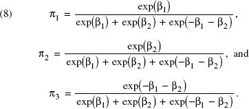
\begin{matrix} π_{1} = \frac{\exp (β_{1})}{\exp (β_{1}) + \exp (β_{2}) + \exp (- β_{1} - β_{2})}, \\ π_{2} = \frac{\exp (β_{2})}{\exp (β_{1}) + \exp (β_{2}) + \exp (- β_{1} - β_{2})}, and \\ π_{3} = \frac{\exp (- β_{1} - β_{2})}{\exp (β_{1}) + \exp (β_{2}) + \exp (- β_{1} - β_{2})} . \end{matrix}

(8)

Inverting these formulas for each draw r = 1, …, R from the prior distribution of the probabilities, we compute the parameters as

\begin{matrix} β_{1}^{r} = \frac{2}{3} \ln π_{1}^{r} - \frac{1}{3} \ln π_{2}^{r} - \frac{1}{3} \ln π_{3}^{r}, and \\ β_{2}^{r} = - \frac{1}{3} \ln π_{1}^{r} + \frac{2}{3} \ln π_{2}^{r} - \frac{1}{3} \ln π_{3}^{r} . \end{matrix}

(9)

This way, we obtain draws of the parameters from the prior distribution that we use in the Bayesian design procedure as described previously. Notice the interesting property of the expressions in Equation 9 that they are invariant to multiplication of π^r_l by a scalar. Consequently, even if the managers' subjective probability estimates do not sum to one, we do not need to normalize them.

Comparison of Design Efficiency

We construct a Bayesian design and a design according to HZ's procedures (but using our algorithms). These designs have 15 choice sets with two alternatives each. In our comparison, we want to establish the effect of eliciting prior information from managers and using that in the Bayesian design. Therefore, we did not want to use the elicited prior information in constructing the HZ-type design and needed to set values for the parameters in that design. We specified them in a way that is analogous to what was proposed by HZ. These parameter values are shown in the second column of Table 4. We believe they are intuitive and appropriately reflect the signs that we expect for the coefficients. Obviously, other choices are possible. The prior parameter estimates, obtained as the median of the minimax subjective probability bounds obtained from the managers, are presented in the third column of Table 4; the fourth column provides the 95% credible interval. Not all the prior estimates obtained from the managers are intuitive, possibly reflecting the managers' difficulty in expressing subjective probabilities formally. The constructed designs are presented in Table 5.

Table 4

PRIOR VALUES, PARAMETER ESTIMATES, AND STANDARD ERRORS

				Estimates of Parameters and Standard Errors
	Prior Parameters			HZ-Type Design		Bayesian Design
Coefficients	HZ-Type Design	Bayesian Design	95% Interval	Parameters	Errors Standard	Parameters	Errors Standard
Location1	-1.0	.272	(.141, .802)	.598	.098	.559	.059
Location2	-1.0	-.617	(-1.683, -.350)	-.872	.114	-.706	.082
Period1	-1.0	-.291	(-1.336, -.331)	-.674	.111	-.652	.058
Period2	.0	-.510	(-1.336, .368)	.000	.053	.111	.062
Activities1	-1.0	.007	(-.035, .270)	.004	.088	-.087	.045
Activities2	-1.0	-.303	(-.828, -.217)	-.313	.104	-.213	.056
Clubs1	-1.0	.649	(.421, 1.338)	.011	.112	-.277	.070
Clubs2	.5	.190	(-.191, .310)	.181	.078	.487	.053
Price1	1.0	-.331	(-.528, -.244)	.597	.111	.452	.056
Price2	.0	.368	(.234, .651)	-.051	.050	-.011	.052

Table 5

DESIGNS USED IN THE EMPIRICAL APPLICATION

		Standard Design					Bayesian Design
		Attributes					Attributes
Choice Set	Profile	1	2	3	4	5	1	2	3	4	5
1	I	3	2	1	2	3	1	3	1	2	3
	II	1	3	3	1	2	3	1	3	1	2
2	I	2	1	2	3	2	1	1	1	3	2
	II	1	3	1	1	3	3	2	2	1	3
3	I	1	1	1	3	1	3	3	1	3	1
	II	2	3	2	2	2	1	1	2	2	3
4	I	3	1	3	1	3	2	1	3	1	3
	II	2	2	2	2	1	1	3	2	2	1
5	I	2	1	3	2	3	2	2	1	2	2
	II	1	2	2	3	1	1	3	3	3	1
6	I	3	2	1	3	1	1	2	3	1	1
	II	1	3	3	2	3	3	3	1	3	3
7	I	2	2	3	1	2	1	2	1	1	2
	II	1	3	1	2	1	2	3	3	2	1
8	I	1	1	3	2	2	2	3	1	1	2
	II	3	3	2	1	3	3	2	3	2	3
9	I	3	2	1	1	2	1	1	3	3	2
	II	2	3	2	3	1	2	2	1	1	1
10	I	1	3	2	2	2	2	3	3	2	2
	II	2	1	3	1	1	1	1	2	1	1
11	I	2	2	1	2	1	3	2	1	2	1
	II	3	1	2	3	3	2	3	2	1	3
12	I	3	1	1	1	1	3	1	2	2	1
	II	1	2	3	3	3	1	2	3	3	3
13	I	2	3	1	3	2	2	3	2	3	2
	II	3	1	2	2	3	3	1	1	2	3
14	I	1	2	3	1	1	2	1	1	1	1
	II	3	1	1	3	2	3	2	2	3	2
15	I	3	1	2	1	2	1	2	3	2	2
	II	2	3	1	3	3	3	1	2	3	3

On the basis of the two designs, a paper-and-pencil conjoint choice questionnaire was developed. The choice sets from both designs were mixed in the same questionnaire, in randomized order, so that the questionnaire contained 30 two-alternative choice sets. A sample of current membership card owners was selected; usable responses were obtained from 58 subjects (undergraduate students of marketing). The estimates of the parameters from the two separate designs and their standard errors are presented in Table 4.

Notice that the prior estimates based on the managers' beliefs are not close to the estimated values in all cases; in particular, the estimated coefficients of Clubs1 and Price1 are substantially outside of the 95% credible interval. This indicates that the managers estimated the percentage of subjects that chose that product to be lower than for the reference level (attribute level 3), but it was higher in the sample. The D_P-errors of the standard and Bayesian designs are .31 and .27, respectively, so that the Bayesian design is approximately 13% better in this application. This is corroborated by an examination of the estimated asymptotic standard errors in Table 4. For two parameters, the standard error estimates obtained from the Bayesian design are the same or slightly larger; for the other parameters, the asymptotic standard errors are 30%–50% lower. In addition to yielding different precision, the parameter estimates of the two designs are also different. Because both designs provide consistent estimates, these differences are due to chance fluctuations. However, because the standard errors for the HZ-type design are larger, the probability that these estimates are farther from the true ones is larger. We observe substantial differences in the estimates for six of ten coefficients—in particular for Period2, Activities1, Clubs1, and Clubs2 and to a lesser extent Activities2 and Price1. These differences in coefficients may have important implications if management wants to implement the results of the study in designing a new membership card. For example, for the Clubs attribute, on the basis of the standard design, management may conclude that differences in customer preference for the three levels are negligible and opt for the simplest, low-cost level. The estimates from the Bayesian design show, however, that there is a strong preference for Clubs2. The probability of constructing a suboptimal product from the standard design is substantially larger than from the Bayesian design results, which is clearly undesirable.

We also compare the two designs using the measures employed in the Monte Carlo study, as presented in Figure 4. The parameter estimates presented in Table 4 have a computed standard deviation from the prior values (Table 4) of .47.⁵ Figure 4 shows that the percentage reduction in the number of subjects a researcher expects to obtain through the Bayesian design for a standard deviation of .47 from the true parameters is approximately 35%, so the actual reduction of 13% we happened to observe in our sample is on the low end. Figure 4 is constructed on the basis of the standard and the Bayesian designs and the prior estimate of the parameter, and this enables us to predict the efficiency of the Bayesian design compared with the standard design. For example, if the true parameter is at a distance corresponding to standard deviations between 3 and 5 from the prior values (computed on the basis of the Euclidean distance), we expect that the Bayesian design needs 10%–14% fewer subjects. As the true value gets closer to the prior estimate, the measure in Figure 4 improves dramatically. This is to be expected, because the more precise the prior estimate, the more efficient is the Bayesian design constructed from it.

This number is given by the ratio of the Euclidean distance of the prior estimates from the true value and the average Euclidean distance of univariate normal random 10-vectors from the origin, which is 3.085.

Figure 4

PERCENTAGE REDUCTION OF SUBJECTS NEEDED FOR THE BAYESIAN DESIGN COMPARED WITH THE STANDARD DESIGN WITH THE SAME EFFICIENCY IN THE APPLICATION

Comparison of Predictive Validity

Predictive validity has been of eminent importance in the evaluation of conjoint models in practice. Although the design-generating procedures aim at improving the efficiency of the estimates, not the predictive capacity of the estimated models, improved efficiency will translate into better expected predictive validity to a certain extent, as we show theoretically and empirically. The criterion we use for assessing the predictive validity of the designs is the expected mean square error (EMSE) of the choices in holdout choice sets. We use the EMSE, because it is not based on the point estimates but takes the entire distribution of the coefficients into account. Formally,

{EMSE}_{D} = {\int [p ({\hat{β}}_{D}) - n]}^{'} [p ({\hat{β}}_{D}) - n] f ({\hat{β}}_{D}) d {\hat{β}}_{D},

(10)

where D = S or D = B; EMSE_S and EMSE_B denote the EMSE of the predicted choice probabilities of the standard and Bayesian designs, respectively; n is the vector of choice frequencies in the holdout choice sets; $p ({\hat{β}}_{D})$ is the corresponding vector of predicted probabilities computed for parameter values $β = {\hat{β}}_{S}$ or ${\hat{β}}_{B}$ according to Equation 2; and $f ({\hat{β}}_{D})$ is the distribution of the estimates. It can be seen from Equation 10 that if the distribution of the estimates $f ({\hat{β}}_{D})$ is more concentrated around the mean, as we expect for the Bayesian design, and the Bayesian parameters are more precise, the EMSE will be smaller. The expectations in Equation 10 can be approximated by averaging over a large number of draws from the distribution of the estimates, as is done for the D_B-error as explained after Equation 6. We approximate these distributions by the asymptotic distribution, which is normal, using the corresponding point estimates for the mean and variance. We use the choices of the respondents in a holdout design consisting of five choice sets, each of which has two alternatives in the empirical application. The numerical values obtained for the EMSEs are EMSE_S = .118 and EMSE_B = .092.

The parameter estimates obtained from the Bayesian procedure have 22% lower expected prediction error than those obtained from the standard procedure. This result adds a new aspect to the design of efficient choice experiments. The Bayesian procedure can produce estimates that are more precise in predicting choice probabilities of new profiles, and the magnitude of the improvement obtained from the design is often larger than what has resulted from improvements in the MNL model itself.

Conclusion and Discussion

Few will contest that managers have relevant knowledge on the behavior of their customers. It therefore may be surprising that managers' subjective beliefs have hardly been used in conjoint experiments. Whereas managers are routinely consulted by market researchers to select the attributes and levels for a conjoint (choice) experiment, the potential of using their beliefs about the attractiveness of attribute-level combinations to customers has remained largely untapped. By designing conjoint experiments based on managers' subjective beliefs, we have addressed the long-standing circular problem that in order to design an experiment to estimate choice model parameters, those parameters need to be known. Bayesian theory enables us to construct designs that have higher efficiency at parameter values that are judged likely by managers. In our empirical illustration, not only did a Bayesian design-generating procedure produce choice designs that resulted in lower estimated standard error than procedures proposed heretofore, but it also provided higher predictive validity. The increased efficiency of the Bayesian design can be decomposed into two components. First, there is the efficiency gain due to incorporating the beliefs of the managers on the choice probabilities of products that possess certain attribute levels, and second, an improvement arises from accommodating managers' uncertainty about the values of those probabilities in the population.

Our study reveals that accurate elicitation of uncertainty is an important issue, in particular with regard to the overconfidence effect. We have made an attempt to alleviate overconfidence in three ways. First, we have used an elicitation procedure that stimulates respondents to state their true beliefs and minimizes overconfidence. Second, we have combined the subjective confidence bounds of several managers using a minimax rule, so that a parameter value that is considered plausible by any of the managers is included in the confidence set. Third, we have taken the resulting confidence set of the parameters as holding with 95% certainty. All of these procedures produce a relatively wide plausible interval for the parameters, which improves the efficiency of the designs. However, the procedures for elicitation (Van Lenthe 1993) and combination (Almond 1996) of belief intervals from several judges need more study. Further research should aim at producing elicitation procedures that enable similar contexts to be invoked for the management judgments and consumer choice tasks, which would ensure maximal congruity between the two (Schwartz and Bohner 2001). Our procedure to produce the prior parameter distribution from subjective probability judgments should be further improved and its sensitivity to several aspects, such as the assumed normal prior distribution of the probabilities, investigated.

Then, the Bayesian design-generating procedure can be extended in several directions. First, effective design-generating algorithms need to be developed that can also be used to determine optimal designs that include a base or no-choice alternative. This problem is important because these types of designs are popular in the conjoint choice literature. Second, following other design-generation procedures currently provided in the literature, we consider the size of the choice set to be fixed by the researcher before design construction. It may be desirable to include the size of the choice set in design construction. However, presently this is hampered by the combinatorial explosion of the designs to be searched over, and the issue awaits the development of better optimization algorithms. Third, the relabeling, swapping, and cycling algorithms can be further improved, for example, through the application of genetic or data-correcting algorithms (Goldengorin and Sierksma 1999). The possibility of implementing such procedures for our designs needs further investigation. Fourth, we believe it is desirable to investigate further the performance of procedures on the basis of different efficiency measures derived from the information matrix. Fifth, we wish to mention the possible extension of our method to the design of logit models that deal with consumer heterogeneity, such as the mixed logit, the latent class logit, or the hierarchical Bayes logit models (Wedel et al. 1999). The construction of optimal designs for the models that include heterogeneity, analogous to the designs proposed by Lenk and colleagues (1996), has not yet been addressed and poses interesting yet computationally intensive problems.

Footnotes

Simple Numerical Example

In this Appendix, we present a simple numerical example of constructing a Bayesian design by eliciting prior information from managers. For this purpose, we consider a small design with three choice sets, each having two alternatives. The alternatives have two attributes: Attribute 1 at three levels denoted 1, 2, and 3, coded [1 0], [0 1], and [-1 −1], respectively, and Attribute 2 at two levels, 1 and 2, coded −1 and 1. We present our algorithm in the following seven steps.

References

Almond

Russel G.

(1996), Graphical Belief Modeling. London: Chapman and Hall.

Atkinson

Anthony C.

, and Donev

Alexander N.

(1992), Optimum Experimental Designs. London: Oxford.

Berger

James O.

(1985), Statistical Decision Theory and Bayesian Analysis. New York: Springer Verlag.

Bunch

David S.

, Louviere

Jordan J.

, and Anderson

Don

(1994), “A Comparison of Experimental Design Strategies for Multinomial Logit Models: The Case of Generic Attributes,” working paper, Graduate School of Management, University of California at Davis.

Chaloner

Kathryn

, and Verdinelli

Isabella

(1995), “Bayesian Experimental Design: A Review,” Statistical Science, 10 (3), 273–304.

Goldengorin

Boris

, and Sierksma

Gerard

(1999), “The Data-Correcting Algorithm for the Minimization of Supermodular Functions,” Management Science, 45 (November), 1539–52.

Huber

Joel

, and Zwerina

Klaus

(1996), “The Importance of Utility Balance in Efficient Choice Design,” Journal of Marketing Research, 33 (August), 307–17.

Kuhfeld

Warren F.

, Tobias

Randall D.

, and Garratt

Mark

(1994), “Efficient Experimental Design with Marketing Research Applications,” Journal of Marketing Research, 31 (November), 545–57.

Lazari

Andreas G.

, and Anderson

Donald A.

(1994), “Designs of Discrete Choice Experiments for Estimating Both Attribute and Availability Cross Effects,” Journal of Marketing Research, 31 (August), 375–83.

10.

Lenk

Peter J.

, DeSarbo

Wayne S.

, Green

Paul E.

, and Young

Martin R.

(1996), “Hierarchical Bayes Conjoint Analysis: Recovery of Partworth Heterogeneity from Reduced Experimental Designs,” Marketing Science, 15 (2), 173–91.

11.

Lichtenstein

, Fischhoff

, and Phillips

L.D.

(1982), “Calibration of Probabilities: The State of the Art to 1980,” in Judgement Under Uncertainty: Heuristics and Biases, Kahneman

Daniel

, eds. Cambridge, UK: Cambridge University Press, 306–34.

12.

Lindsey

James K.

(1996), Parametric Statistical Inference. London: Oxford.

13.

Louviere

Jordan J.

, and Woodworth

George

(1983), “Design and Analysis of Simulated Consumer Choice or Allocation Experiments: An Approach Based on Aggregate Data,” Journal of Marketing Research, 20 (November), 350–67.

14.

Pilz

Jürgen

(1991), Bayesian Estimation and Experimental Design in Linear Regression Models. Chichester, UK: John Wiley & Sons.

15.

Savage

Leonard J.

(1976), “On Rereading R.A. Fisher,” Annals of Statistics, 4 (3), 441–500.

16.

Schwartz

Norbert

, and Bohner

Gerd

(2001), “The Construction of Attitudes,” in Blackwell Handbook of Social Psychology: Intraindividual Processes, Tesser

, and Schwartz

, eds. Oxford, UK: Blackwell.

17.

Shafer

Glenn

(1982), “Belief Functions and Parametric Models,” Journal of the Royal Statistical Society, B, 44 (3), 322–52.

18.

Silvey

Samuel David

(1980), Optimal Design: An Introduction to the Theory for Parameter Estimation. London: Chapman and Hall.

19.

Van Lenthe

Jelle

(1993), “ELI: An Interactive Elicitation Technique for Subjective Probability Distributions,” Organizational Behavior and Human Decision Processes, 55 (3), 379–413.

20.

Wedel

Michel

, Kamakura

Wagner A.

, Arora

Neeraj

, Bemmaor

Albert

, Chiang

Jeongwen

, Elrod

Terry

, Johnson

Rich

, Lenk

Peter

, Neslin

Scott

, and Poulsen

Carsten Stig

(1999), “Discrete and Continuous Representation of Heterogeneity,” Marketing Letters, 10 (3), 217–30.

21.

Yates

J.F.

, Zhu

, Ronis

D.L.

, Wang

D.F.

, Shinotsuka

, and Toda

(1989), “Probability Judgement Accuracy: China, Japan and the United States,” Organizational Behavior and Human Decision Processes, 43 (2), 145–71.

22.

Zacks

(1977), “Problems and Approaches in Design of Experiments for Estimation and Testing in Non-linear Models,” in Multivariate Analysis, IV, Krishnaiah

D.R.

, ed. Amsterdam, The Netherlands: North Holland, 209–23.