Using Multimarket Data to Predict Brand Performance in Markets for Which No or Poor Data Exist

Abstract

The authors show how multimarket data can be used to make predictions about brand performance in markets for which no or poor data exist. To obtain these predictions, the authors propose a model for market similarity that incorporates the structure of the U.S. retailing industry and the geographic location of markets. The model makes use of the idea that if two markets have the same retailers or are located close to each other, then branded goods in these markets should have similar sales performance (other factors being held constant). In holdout samples, the proposed spatial prediction method improves greatly on naive predictors such as global-market averages, nearest neighbor predictors, or local averages. In addition, the authors show that the spatial model gives more plausible estimates of price elasticities. It does so for two reasons. First, the spatial model helps solve an omitted variables problem by allowing for unobserved factors with a cross-market structure. An example of such unobserved factors is the shelf-space allocations made at the retail-chain level. Second, the model deals with uninformative estimates of price elasticities by drawing them toward their local averages. The authors discuss other substantive issues as well as future research.

Most large consumer goods manufacturers wish to monitor sales performance of their brands in a variety of regional markets. To accommodate this desire, the leading market research providers, such as Information Resources Inc. (IRI) or ACNielsen, collect multimarket time-series data of brand performance through complex data-collection systems. These multimarket data are now widely available to both practitioners and academicians, but they pose several new challenges.

First, in the United States, many locations are left unsampled because of obvious economic constraints in collecting and handling complete time-by-market data. The exclusion of many locations from the spatial sample poses a missing data problem for managers of national brands who frequently make decisions on the basis of local demand conditions (Hoch et al. 1995). We propose to solve this problem through spatial prediction.

Second, and not unrelated, strong dependencies across the sampled markets can and do occur. These dependencies raise new issues about how to model multimarket data. At least in marketing, modeling approaches rarely broach on the subject of cross-sectional or spatial dependencies of data from multiple locations.

Perhaps as a result, and despite the familiarity of marketing practitioners and academicians with the extrapolation of stochastic processes in time, spatial prediction has remained unstudied in our field. Both prediction problems share the same underlying philosophy: The goal is to determine the sample points that are most informative about the behavior of the process at prediction points. The main distinction is that stochastic processes in space are multidimensional and do not have a clear or particular ordering. In contrast, stochastic processes in time are defined over one single dimension of interest—time itself—with a natural and clear directional ordering. Because of these differences, the spatial prediction problem is nonstandard.

In this article, we demonstrate how to model spatial dependence across markets, and we offer a perspective on how to make spatial predictions. Our contribution is intended to be both methodological and substantive. Methodologically, we first make an existing spatial prediction method, called kriging (pronounced KREE-ging), operational in marketing and test its performance. Our spatial prediction approach is based on a model that can be calibrated on spatiotemporal data. It is estimated using Markov Chain Monte Carlo (MCMC) methods.

Second, we also contribute methodologically to the spatial prediction problem by using the presence of the same retailers in multiple markets to construct a measure of market similarity. In other words, whereas traditional spatial prediction methods use purely distance-based metrics, we develop a model that also captures the impact of retailer territories on the multimarket data. In the process, we (1) obtain a cross-market covariation structure that is more flexible and provides a better representation of the data than purely distance-based approaches and (2) offer a measure of the importance of the U.S. retail structure in explaining the cross-sectional variation in the data, while controlling for purely spatial (i.e., distance-based) effects in a variance decomposition model.

Substantively, we aim to shed some light on the determinants of the cross-sectional differences in sales performance for nationally distributed brands. For the brands considered, market performance measures, such as market shares and sales velocity, differ greatly across the 64 markets sampled by IRI, despite the product homogeneity that characterizes the categories under analysis. To investigate possible sources for these cross-sectional differences, we allow for distance effects and retailer effects on (1) model constants, (2) observed dynamic effects (e.g., due to price), and (3) unobserved dynamic effects (e.g., due to unobserved retailer behavior).

Our analysis offers the following conclusions: First, the territories of retailers in the U.S. are “shingled” in the sense that retailers' territories neither perfectly overlap nor are completely separated. There are, in other words, no truly isolated markets in the network of U.S. retailers. Second, the structure of the U.S. retail industry accounts for a large portion of the cross-market variance of the data, even in the presence of competing distance-based spatial structures. Third, estimates of price elasticities are more efficient (and more reasonable) when the spatial nature of the data is accounted for. Finally, for both performance measures, kriging methods outperform naive predictors, such as local averages, across holdout samples of various sizes and spatial structures (e.g., geographic region versus random locations). This result appears especially true when the holdout sample is large and the estimation sample is small, which demonstrates the usefulness and power of these new approaches.

The remainder of this article is structured as follows: In the next section, we discuss a set of marketing problems that researchers may fruitfully address through spatial prediction. Then, we develop our model for spatiotemporal data and formalize the spatial predictor. In the following section, we focus on spatial covariance models and a model of the U.S. retailing industry. We then provide the empirical analysis and conclude with future research and managerial implications.

Multimarket Data

Temporal and Spatial Components in Multimarket Data

Syndicated market data for the grocery industry are collected in the United States for a multitude of geographic markets, often defined as a metropolitan area or a part of a state. These data are generally correlated across both time and locations. Time dependence can be caused by brand loyalty, inertia within the distribution channel, the use of heuristic decision rules (e.g., history based pricing), or the seasonal nature of some products. Spatial dependence, in contrast, can be caused by the economic agents in the distribution channel (e.g., retailers) that are common to multiple markets, by climate-dependent demand of some product categories, or by a nonrandom distribution of consumer types.

Given the pervasiveness of these three factors, correlation of demand across geographic markets is likely to be the norm and not the exception in multimarket data. Yet not much academic work has explicitly accounted for these dependencies and their effects on inference. To fill this hiatus in the literature, we classify spatial dependence into different types on the basis of the duration and the reach of the spatial effects (see Table 1). First, in terms of duration, spatial dependence may apply to either constant or dynamic data components.

Table 1

Examples of Effects on Brand Performance in Multimarket Data

Spatial Effects	Time Effects
Spatial Effects	Dynamic	Constant
Short range (e.g., local market) Medium range (e.g., retailer trade area) Long range (e.g., national market)	Behavior of independent stores Retailer-level pricing decisions Manufacturer supply constraints Climate	Consumer type distributions Retailer-level distribution decisions Order-of-entry effects

Second, spatial dependencies may die out over a short (e.g., local market), a medium (e.g., retailer trade area), or a long range in space (e.g., the domestic U.S. market). The spatial dependencies induced by the distribution of consumer types and the behavior of independent retailers are both short-range dependencies, though one type of dependency is constant whereas the other changes over time.

At the medium-range level, the effects of retailer-level pricing and promotion decisions are an example of dynamic effects with a regional character. The effects of retailer-level distribution decisions (adoption)—which are made less frequently than promotion decisions—cause a more constant component with regional structure.

Finally, manufacturer supply constraints, climate variations, and order-of-entry effects may also lead to spatial dependencies that hold over longer ranges (such as the entire domestic U.S. market). For example, order-of-entry decisions by manufacturers reflect unobserved market conditions and transportation and distribution costs, among other factors, at the time of the product launch. To the extent that such order-of-entry effects have permanent effects on the data, they may give rise to larger-share “home-markets” and lower-share “distant markets”; that is, such order-of-entry effects may cause a long-range spatial dependence in the data that is more or less constant. In contrast, supply constraints and climate variations give rise to spatial dependencies that vary over time.

This classification of the spatial dependencies provides the basic framework we use to both understand and model spatial phenomena. Next, we present some marketing applications that can benefit from the modeling of these spatial phenomena and introduce our modeling and prediction approaches.

Applications of Spatial Analysis to Marketing

Collecting, handling, and maintaining full time-by-space data over all relevant cross-sectional units is both cost prohibitive and likely subject to diminishing marginal returns in information content. Therefore, we believe that spatial prediction methods may provide great benefits to market researchers in situations in which detailed knowledge exists on selected cross-sectional units and information is required about other cross-sectional units. Store audits and shelf-space audits, market tests of new products, hit rate predictions for direct marketing companies, and micromarketing studies are some examples of possible applications in which we may observe such benefits. The only difference between these examples is how we define the cross-sectional units.

For example, store audits or shelf-space audits give detailed information about merchandizing activity or shelf-space allocation for a subset of stores. Spatial prediction can then help predict store execution of promotions or shelf-space allocations for unsampled stores.

Customer records, which include Zip code information, owned by catalog, Internet, or direct-marketing companies represent another example of a sparsely sampled cross-section of data. These companies have an interest in knowing, for example, the a priori hit rate of mailings to potential customers in certain Zip code areas (see, e.g., Steenburgh, Ainslie, and Engebretson 2001). By means of spatial methods, it is generally possible to interpolate such information from hit rate data of current customers given their location.

Micromarketing, the fine-tuning of the marketing mix to local markets (see Hoch et al. 1995), provides yet another example. Spatial prediction can be helpful in forecasting, say, the responses to price promotions in unsampled markets from the corresponding responses in sampled markets. These forecasts are fundamental input to any micromarketing decision process.

Finally, the proposed spatial prediction methods are also beneficial when a given market, though sampled, provides “poor” (i.e., imprecise) information. This is because we use a Bayesian approach that allows for the influence of precise information from close markets during estimation.

Modeling and Prediction Approach

A Model of Market-by-Time Panel Data

The purpose of our modeling work is to investigate spatial dependence of brand performance across regional markets. It is our goal to capture the impact of spatial variables that are either time-invariant, as in the case of demand constants, or dynamic, as in the case of price effects. To do so, we allow demand intercepts, prices, and price responses to be spatially distributed. We also allow for a stochastic term that is both spatially and time dependent to capture other unobserved spatial effects. We have adopted a log-log formulation for the demand model because such a formulation provides direct estimates of price elasticities, which may be compared across markets.

Assume that we sample N locations, for T time periods. Our basic demand model is

\begin{matrix} y_{t} = \tilde{α} + diag ({\tilde{p}}_{t}) β+ e_{t}, & t = 1, \dots, T \\ e_{t} = p_{y} e_{t - 1} + η_{t}, \end{matrix}

(1)

where y_t is an N × 1 vector of log-demands for all the markets at time period t,

{\tilde{p}}_{t}

is an N × 1 vector of log-prices, and diag(·) represents the operator that transforms a vector into a diagonal matrix (i.e., diag(

{\tilde{p}}_{t}

) is an N × N diagonal matrix of log-prices). The element

\tilde{α}

is an N × 1 vector of intercepts, and β is an N × 1 vector of price elasticities. The scalar ρ_y is an autoregression effect for the N × 1 vector of demand error terms, e_t, and η_t is an N × 1 vector of zero-mean time-independent stochastic terms. The autocorrelation in e_t can be due to inertia of manufacturers, retailers, consumers, or any other channel participant.

Using the within-market means 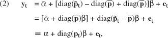${\bar{p}}_{i}$ of the log-prices, p_it, we orthogonalize the demand system by rewriting it as follows:

\begin{matrix} y_{t} & = \tilde{α} + [diag ({\tilde{p}}_{t}) - diag (\bar{p}) + diag (\bar{p})] β + e_{t} \\ = [\tilde{α} + diag (\bar{p}) β] + diag ({\tilde{p}}_{t} - \bar{p}) β + e_{t} \\ \equiv α + diag (p_{t}) β + e_{t}, \end{matrix}

(2)

where

\bar{p}

is an N × 1 vector containing the means of log-prices for all markets, and p_t is an N × 1 vector of demeaned log-prices.

As a result, the transformed model factors the data into three separate “bins,” each of which may be subject to spatial dependencies: (1) constant demand effects, α; (2) observed time-varying price effects, diag(p_t)β; and (3) unobserved time-varying effects, e_t, which are autoregressive transient shocks. If so desired, the original demand constants, $\tilde{α}$ , can be easily recovered using the estimated values of α, β, and the means of log-price.

If we had access to the actual market prices for all markets, sampled and unsampled, spatial predictions would require only the estimates of the unknowns in Equation 2 and the variance–covariance structures of all spatial variables. In general, however, price knowledge is absent for unsampled locations. In such cases, before we predict demand, we must first predict prices or, more specifically, demeaned log-prices. Therefore, we specify the following model for the demeaned log-prices (making use of the mean of p_t being zero)

\begin{matrix} p_{t} = 0 + v_{t} \\ v_{t} = p_{p} v_{t - 1} + ξ_{t}, \end{matrix}

(3)

where the scalar ρ_p is an autoregression effect for the N × 1 vector of price error terms, v_t, and ξ_t is an N × 1 vector of zero-mean time-independent stochastic terms. Although this model appears rudimentary, it is necessary for the spatial prediction of prices.

Spatial Processes

To predict brand performance for M unsampled locations, we now allow some components of our model to be spatially distributed and specify their spatial processes. In Equation 2, we allow for three potential sources of spatial structure: (1) the demand constants, α; (2) the price-elasticities, β; and (3) the random shocks, e_t, through the time-independent shocks η_t. We also allow the demeaned log-prices in Equation 3 to be spatially distributed through the time-independent random shocks ξ_t. We assume that these spatial variables follow (different) second-order stationary spatial processes in ℝ², that is, spatial processes that satisfy the following two properties (using α to illustrate):

{\begin{matrix} E (α_{i}) = Z_{αi} φ \end{matrix}}_{α}, = \forall i and cov (α_{i}, α_{i'}) = Λ_{α} (d_{ii'}, θ_{α}),

(4)

where i and I′ designate markets, Z_αi is a vector of covariates, and φ_α is the corresponding vector of parameters. The notation Λ_α(d_ii′, θ_α) reflects that the covariance is a function of a parameter vector, θ_α, and of location differentials, d_ii′, such as the distance or the direction between location pairs.¹ Therefore, the covariance function does not depend on absolute location of i or i′. If this function depends only on distance, it is called “isotropic.” If it also depends on the direction of the vector connecting the location pair {i, i′}, it is called “anisotropic.” We abbreviate the notation for the full variance–covariance matrix Λ_α(d, θ_α) by Λ_α.

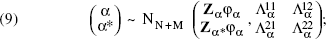
The same principle is used frequently in temporal dependence. For example, the standard AR(1) process has a variance–covariance function that is dependent on time differences (the equivalent to d_ii′) and on an autocorrelation parameter (the equivalent to 8).

As a result of the second-order stationarity assumption, the cross-sectional structure—which is measurable through the N sample points—will hold over all N + M locations. For each of the spatial components in the model, we use a joint Normal distribution over N + M variates. That is, we posit the following:

\begin{matrix} {(α^{'} α^{*'})}^{'} \sim N_{N+M} (Z_{α} φ_{α}, Λ_{α}), \end{matrix}

(5)

\begin{matrix} \begin{matrix} {(β^{'} β^{*'})}^{^{'}} \sim N_{N+M} (Z_{α} φ_{β}, Λ_{β}), \end{matrix} \end{matrix}

(6)

\begin{matrix} \begin{matrix} \begin{matrix} {(η_{t}^{'} η_{t}^{*'})}^{'} \sim N_{N+M} (0, Λ_{η}), \end{matrix} \end{matrix} \end{matrix} and

(7)

\begin{matrix} \begin{matrix} \begin{matrix} {(ξ_{t}^{'} ξ_{t}^{*'})}^{'} \sim N_{N + M} (0, Λ_{ξ}), \end{matrix} \end{matrix} \end{matrix}

(8)

where α^*, β^*, η_t^*, and ξ_t^* are M × 1 vectors of the demand constants, price elasticities, demand shocks, and price shocks for the unsampled markets, respectively. Elements Z_α and Z_β are covariates, and φ_α and φ_β are vectors of corresponding parameters. We assume that the unobserved components of the spatial variables are conditionally independent from one another. This implies the assumption that the unobserved components of one spatial variable are conditionally uninformative about the unobserved components of other spatial variables.

The variance–covariance structure of the stacked stochastic terms from Equation 1, e = [e′₁ … e′_T]′ for all sampled and unsampled markets, is a (M + N)T square matrix equal to Ψ_y ⊗ Λ_n (for a brief overview of some proofs, see also Appendix A). The element Ψ_y is the standard variance–covariance matrix for an AR(1) process with autoregressive parameter ρ_y and with unit variance in the innovation terms (see Judge et al. 1985, p. 284). Similarly, the variance–covariance matrix of the corresponding stacked price error terms, v, is Ψ_p ⊗ Λ_ξ, where Ψ_p is the variance–covariance matrix of an AR(1) process with autoregressive parameter ρ_p and unit variance in the innovation terms. The exact modeling of the variance–covariance matrices Λ_α, Λ_β, Λ_η, and Λ_ξ is discussed subsequently.

Spatial Prediction or Kriging

Assuming that estimates for the model exist, we now address how these can be used for spatial prediction. We assume that we want to predict the process for some market j, where j = N + 1, …, N + M, at a time period t, for t = 1, …, T.² We need to spatially predict four (conditionally) independent components of the model: the constants α_j*, the price elasticities β_j*, the random components e_jt*, and the random components v_jt*. The method of spatial prediction is identical for α_j* and β_j* on the one hand, and for e_jt* and v_jt* on the other.

We do not consider here the case of predicting out of both the spatial sample and the time sample. However, such a case is easy to develop.

Case 1: Prediction of the Demand Constants α_j* and the Price Elasticities β_j*

Consider the case of the demand constants (similar results hold for the price elasticities). For spatial prediction, partition Equation 5 into

(_{α^{*}}^{α}) \sim N_{N+M} (_{Z_{α *} φ_{α}}^{Z_{α} φ_{α}},_{Λ_{α}^{21}}^{Λ_{α}^{11}}_{Λ_{α}^{22}}^{Λ_{α}^{12}});

(9)

then (Searle, Casella, and McCulloch 1992) [α^*|α] is multivariate Normal with

\begin{matrix} E (α^{*} | α) = \end{matrix} \underset{regression mean}{\underset{︸}{Z_{α^{*}} φ_{α}}} + \underset{adjustment for spatial depedence}{\underset{︸}{Λ_{α}^{21} {(Λ_{α}^{11})}^{- 1} (α - Z_{α} φ_{α})}}

(10)

and

\begin{matrix} Λ (α^{*} | α) = Λ_{α}^{22} - \end{matrix} Λ_{α}^{21} {(Λ_{α}^{11})}^{- 1} Λ_{α}^{12} .

(11)

If we estimate φ_α using ${\hat{φ}}_{α}^{GLS} = {[{Z^{'}}_{α} {(Λ_{α}^{11})}^{- 1} Zα]}^{- 1} {Z^{'}}_{α} {(Λ_{α}^{11})}^{- 1} α$ , then the mean of the conditional distribution in Equation 10 is called the “universal kriging predictor” (see Cressie 1993). The first term of this predictor, $Z_{α*} {\hat{φ}}_{α}^{GLS}$ , is the standard generalized regression result. This term ignores the unobserved spatial covariation, Λ_α¹¹, in (α − Z_αφ_α). The second term in the predictor corrects for this correlation and is the conditional expectation of the unobserved stochastic terms, (α* − Z_α*φ_α), given the observed differences (α − Z_αφ_α). Therefore, we can interpret the kriging predictor as an adjusted generalized least squares predictor. Cressie (1993) shows that this predictor has the additional benefit of minimizing the squared prediction error; that is, it is the best linear unbiased predictor.

Case 2: Prediction of the Stochastic Terms e_jt* and v_jt*

As an example, consider the prediction of e_jt* (j = N + 1, …, N + M, t = 1, …, T). This case proceeds in a similar fashion as in the previous case. The main difference is that, given the temporal structure of the stochastic terms, we need to condition our predictions on all NT stochastic terms from our sample, as opposed to only the N contemporaneous stochastic terms, e_t = [e_lt,…,e_Nt]. In Appendix A, we prove that for the prediction of the M × 1 vector e_t* conditional on the full NT × 1 vector e, only the subvector e_t matters, so that

\begin{matrix} E (e_{t}^{*} | e) = Λ_{η}^{21} \end{matrix} {(Λ_{η}^{11})}^{- 1} e_{t}

(12)

and

V (e_{t}^{*} | e) = \frac{1}{1 - ρ_{y}^{2}} [Λ_{η}^{22} - Λ_{η}^{21} {(Λ_{η}^{11})}^{- 1} Λ_{η}^{12}] .

(13)

Similar results hold for the prediction of v_t* (t = 1, …, T).

Some Differences with the Classic Kriging Predictor

Kriging methods require knowledge of the spatial (co)variance structure of the data, as can be seen from Equation 10. In practice, researchers using the classic kriging predictor estimate the cross-sectional covariance using actual observations of, say, α_i for i = 1, …, N.³ After the parameters on which the covariance Λ_α depends, here denoted as θ_α, are estimated, it is simple to estimate the variance–covariance matrix Λ_α(d, θ_α) of the (N + M) random vector [α′ α^*′]′. Researchers can then predict the mean and the variance of the process for the M unobserved markets using Equations 10 and 11.

For alternative empirical methods to estimate the covariogram or covariance function, see Cressie (1993, Ch. 2).

Despite their intuitive appeal, classic kriging methods have some drawbacks that we seek to address with the approach presented in this article. First, although classic kriging infers Λ_α from sampled data, the final predictor does not account for the sampling error in θ_α. This is a general problem affecting any classic kriging application. In contrast, our prediction approach relies on Bayesian methods and constructs a marginal predictive distribution that integrates over the density of all unknown model parameters.

Second, classic kriging models the covariance structure solely on the basis of distance. In marketing contexts, this method is, at best, a reduced-form approach. Instead, in the next section, we derive the spatial structure of the data from first principles. Specifically, we incorporate the spatial organization and an aspect of the behavior of retailers in the variance–covariance model. Doing so, we obtain direction-sensitive patterns of covariation that cannot be represented even with very flexible anisotropic covariance functions.

Finally, in a marketing context, not all variables of managerial interest are directly observable (e.g., α is estimated, not observed). Therefore, cross-sectional prediction of these measures requires the construction of both a measurement and a prediction model. Classic kriging addresses the prediction problem but does not address the issue of measurement. In contrast, our model incorporates both.

Specific Models of Covariation

Components of the Covariance Structure

We model the variance–covariance structure of the unobserved components of the demand constants, Λ_α; of price elasticities, Λ_β; of temporary demand shocks, Λ_η; and of temporary price shocks, Λ_ξ, as mixtures of three independent variance structures that are, respectively, distance based, retailer based, and purely random. Therefore, we postulate that the variance–covariance structure for each spatial variable can be factored into three components such that (using the demand intercepts a as an illustration)

\begin{matrix} Λ_{α} = θ_{α3}^{2} \sum_{Rα} (θ_{α1}) + θ_{α4}^{2} \end{matrix} \sum_{sα} (θ_{α2}) + θ_{α5}^{2} I_{(N+M)},

(14)

where θ_α3, θ_α4, and θ_α5 are all positive unknown parameters. The term

θ_{α3}^{2} Σ_{Rα} (θ_{α1})

represents the retailer component,

θ_{α4}^{2} Σ_{Sα} (θ_{α2})

represents the distance-based component, and

θ_{α5}^{2} I_{(N + M)}

represents a spatially uncorrected variance component. Similar expressions hold for the remaining spatial variables β, η_t, and ξ_t.

The distance-based component of the spatial variance–covariance serves as an approximation to several unobserved variables (e.g., taste, culture, climate) that can be correlated across neighboring markets and can affect the spatial variables.

The retailer-based component accounts for the effects of retailer structure and conduct on the spatial variables. Different mechanisms exist that justify the presence of these retailer-based effects. For example, retailers have control of shelf-space policies and other forms of brand support. Therefore, we expect retailers to affect the baseline sales of the brand (captured in demand constants α or the dynamic sales effects η_t). Retailers also influence the composition of their clientele in terms of price sensitivity with store-format choice and private-label program decisions. Consequently, observed price responses may vary with retailer structure and conduct. Finally, prices themselves are often set at the account level, so we also expect price effects, η_t, to have a retailer structure. Next, we describe in more detail both the spatial and the retailer model of covariation and provide an interpretation for different possible patterns.

Distance-Based Model of Covariation

The typical procedure in selecting a functional form for a distance-based covariogram is to plot the empirical covariogram and choose a valid covariance function that allows for the type of patterns actually encountered in the data (e.g., whether spatial correlations die out, whether there are positive and/or negative correlations, whether there is a need to account for measurement error). Both Cressie (1993) and Journel and Huijbregts (1978) offer an overview of the effects that are usually considered part of the spatial covariance function. In our application, we found that positive correlations dominate between observations that are close together but that negative spatial correlations may occur between observations that are separated by larger distances in space. This would happen when the observations have a tendency (as they do in our data) to be below average on one coast and above average on the other. As a result, we use a covariogram in ℝ² that allows for negative correlations across larger distances.

The choice of a specific functional form that is valid for use as a covariance function is not trivial and depends on the number of spatial dimensions used. For example, for any n-dimensional process, the spatial autocorrelations cannot be less than −1/n (see, e.g., Christakos 1984). Therefore, not all models of covariation in ℝ¹ are valid in ℝⁿ, for n > 1. Valid models in ℝⁿ are, however, valid in spaces with less than n dimensions. Other requirements on valid covariograms exist, and the literature on valid covariograms in ℝⁿ has received much attention in spatial analysis (see, e.g., Christakos 1984; Mantoglou and Wilson 1982; Vecchia 1988; Whittle 1954).

For our empirical analysis, we selected a function that is often used in the spatial sciences as a correlation function in ℝ² and allows for negative correlations. This function is the Bessel function of the first kind and order 0 (see, e.g., Christakos 1984; Mantoglou and Wilson 1982; Matern 1986). This correlation function is parameterized by a single parameter that controls the range of going from positive to negative correlation and looks like a dampened oscillation in distance. It is also a simple and standard function in most econometric software.

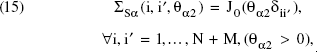
Formally, each (i, i′) element of the matrix Σ_Sα(θ_α2), which forms the distance-based variance–covariance matrix, is defined as follows:

\begin{matrix} \sum_{Sα} ({i,i}^{'}, θ_{α2}) = J_{0} (θ_{α2} δ_{ii'}), \\ \forall {i,i}^{'} = 1, \dots, N + M, (θ_{α2} > 0), \end{matrix}

(15)

where δ_ii′ is the distance between location i and location i′, and J₀ is the Bessel function of the first kind and order 0. In Figure 1, we illustrate the shapes of the Bessel function for two representative values of θ_α2. Distance is expressed in rads (see also the empirical section) spanning the distance between the East Coast and the West Coast.

Figure 1

Two Patterns of Distance-Based Correlations Generated by the Bessel Function

Retailer Model of Covariation

To model the covariation structure across markets due to retailer location and conduct, we assume that a component of retailer policies is common to the level of a retail account. The retail account is generally the unit at which retailers make decisions. It is either a portion of the retail chain—typically if the retailer is spread over multiple states—or the entire retailer.

Define a K × (N + M) matrix H of retail structure containing the share of all-commodity volume (ACV) for each retailer account r (r = 1, …, K) in each sampled and unsampled market i (i = 1, …, N + M). Columns in H sum to one, and a typical element H(r, i) is a number from 0 to 1 that indicates the relative size of retailer r in market i.

In addition, we construct an asymmetric retailer influence matrix W of size K × K. This matrix lists in each row, that is, for each retailer, the relative size of all other retailers it competes with directly. Define {C_r} as the set of markets in which retailer r is present; that is, {C_r} is the territory of retailer r. Then, a typical element of W is computed as follows:

W ({r,r}^{'}) = \frac{\sum_{i \in {C_{r}}} ACV (r^{'}, i)}{\sum_{r^{″} \neq r} \sum_{i \in {C_{r}}} ACV (r^{″}, i)} and W (r,r) = 0.

(16)

In other words, W contains, in each row r, the normalized ACV share of each of the other retailers in r's retail territory. Rows of W add to one, and its diagonal is zero. Note that W accounts for differences in market size. For example, W(r, r′) will be higher if the competing retailer r′ is large in big markets than if it is large in small markets.

We assume that the elements in the rth row of W capture the relative competitive influence on r. We illustrate the effect of this influence for the spatial variable α. Suppose a retailer r has an effect on the demand intercepts equal to S_αr. Although this effect is unobservable to the analyst, it is possible to make inferences about the structure that such unobservable effects would cause across space, given the structure of retail territories and retailer conduct. For this purpose, we model the retailer effect on demand intercepts S_αr as a combination of retailer r's idiosyncratic actions and of the competitive influence from the other retailers in r's territory. Vectorizing the retailers' effects S_αr into a K × 1 vector S_α, we then have

\begin{matrix} S_{α} \underset{(K \times 1)}{=} θ_{α1} W S_{α} + υ \Leftrightarrow \\ S_{α} = {(I_{K} - θ_{α1} W)}^{- 1} υ - 1 < θ_{α1} < 1. \end{matrix}

(17)

The K × 1 stochastic vector υ is assumed independent, with mean 0 and variance $θ_{α3}^{2} I_{K}$ , and reflects the idiosyncratic actions of the retailers to support one brand over another. The term θ_α1WS_α represents a local interaction effect reflecting the competitive interaction of retailers. A short way of defining this relation is simply to point out that we allow the spatial variables to be autoregressive across retail territories. The parameter θ_α1 controls the strength and direction of the interaction among retailers in supporting one brand versus another. The strongest form of interaction occurs when θ_α1 approaches 1 or −1. In the first case, retailers locally imitate one another. In the second case, retailers tend not to follow one another. This may happen when retailers vie for locally exclusive distribution of nationally available brands.

We can convert the retailer-level effects on intercepts, S_α, to market-level effects by taking their weighted average, where the weights are the relative size of each retailer in market i. In mathematical notation, the market-level effects due to retailers correspond to the ith element of the vector H′S_α, where H is the matrix of relative size of each retailer in each market (as defined previously). Therefore, the implied variance–covariance structure across markets due to retail structure and conduct is equal to $θ_{α3}^{2} Σ_{Rα} (θ_{α1})$ , such that

\begin{matrix} \sum_{Rα} (θ_{α1}) = H^{'} {(I_{K} - θ_{α 1} W)}^{- 1} {(I_{K} - θ_{α 1} W)}^{- 1}' \end{matrix} H,

(18)

where

θ_{α3}^{2}

is the scale parameter or the variance of the innovations υ. We discuss the different patterns of spatial correlation that this function generates subsequently.

Covariation Patterns

Our parsimonious variance model can capture a wide variety of covariation patterns, depending on alternative mixtures of retailer- and distance-based spatial components. This flexibility results from the distinct features of each component. For example, distance-based spatial effects in our data are long-range, direction independent, and smooth, whereas retailer-based covariation patterns are direction sensitive and show ridges and discontinuities according to the shapes of retail territories. With mixtures of these different components, the model is flexible enough to accommodate the intricate patterns of covariation that can be expected in market performance data.

We consider two specific patterns from the retailer model. First, when there is no retailer interaction but only retailer structure effects (i.e., θ_.1 = 0 and θ_.3 > 0) cross-market dependence is local (see also the next section) and direction dependent. Mathematically, we obtain from Equation 18 that $Σ_{R \cdot} = H^{'} H \equiv H$ , where $H$ has market-specific Herfindahl indices of retailer concentration on the diagonal and cross-products of the retail shares in two markets on the off-diagonals. If this cross-product is zero, no retailer serves both markets, whereas if this product is high, few retailers have high share in both markets. Therefore, cross-market correlation will be present simply because an unobserved component of the spatial variables in retailer-specific and retailer territories spans multiple markets.

Second, when retail interaction and retail structure effects exist (i.e., θ_.1 ≠ 0 and 8 _.3 > 0), both retailer multimarket presence and the interaction among competing retailers explain cross-sectional variability. In addition, retailers indirectly influence one another even when their territories do not overlap, simply because retailers interact with one another. For example, Retailers A and C may not compete head-to-head, because their territories do not overlap. However, A may indirectly influence C, and vice versa, if they have Retailer B as a common competitor. As θ_.1 increases in absolute value, the indirect influence of A on C becomes more important, and retailer dependence extends over larger areas.

Empirical Analysis

Data

In our empirical application, we combine four different data sets. First, we apply the proposed spatial prediction methods to INFOSCAN sales and price data for Mexican salsa and tortilla chips. The raw data, collected by IRI over two years (May 1994 to April 1996) from its sample of approximately 3000 stores in 64 domestic U.S. markets, are at the local market level.

Second, to operationalize the retail structure model, we obtained U.S. retail data from TradeDimension. These data are at the designated market area (DMA) level. A DMA is a geographic area that designates a single advertising market. The continental U.S. market is divided into 205 DMAs, and every county in the United States is a member of one and only one DMA. The retail structure data include account-by-market ACV for all retailer accounts with more than .1% market share. TradeDimension also has the same data at the IRI market level. From these data, we retained the retailers present in more than two markets and with no less than 10% market share in at least one of the markets in which they operate. Thus, we removed from the data retailers that are too small to play a major role in the spatial structure of demand. We also removed the so-called independent retailers. These retailers share the same label but do not correspond to the same decision makers across the markets. In total, this left us with 185 retail chains. These include national discounters such as Wal-Mart and Kmart and retailer chains such as Albertsons, H-E-B, and Vons.

Third, to compute distances, we collected location data for all DMAs and all IRI markets. We computed the location of each DMA from the latitude and longitude coordinates of Zip code centroids and a mapping of Zip codes into DMAs. (The necessary data to make this computation are available from http://www.zipinfo.com.) For the 64 IRI markets, we collected longitude and latitude data using an Internet mapping service (available at http://www.indo.com/distance). Most IRI markets are associated with a single city. In some cases, a single IRI market is defined as either a part of a state or a set of multiple cities. In these cases, we approximated the location of these IRI markets by an interior point. We used the latitude and longitude data (in rads) to compute pairwise market distances (1 rad ≈ 4000 miles at the equator).

Fourth, we collected demographic information for each county in the United States from the Census Bureau's 1994 County and City Data Book. We aggregated these data to the DMA and IRI market level.

Estimation

The combination of the temporal Equations 2 and 3 with the four cross-sectional Equations 5–8 forms a hierarchical model, which we estimate using Bayesian methods. Given the complexity of the model, an MCMC approach is necessary to simulate the posterior and predictive distributions of the variables of interest.

The specification of the priors and the full conditional distributions used in the MCMC algorithm appear in Appendix B. An important feature of this MCMC algorithm pertains to the full conditional distributions of the spatial variables α_i and β_i, for each market i. These conditional distributions combine two sources of relevant information: (1) the time-series data of market i and (2) the values of the spatial variables for the remaining markets. The mixing of these two types of information will depend on the data itself. For example, if the α_is and β_is are spatially dependent, the time series estimates for these parameters will be shrunk to their local averages. This shrinkage is stronger when the within-market data are less informative about the α_is and β_is. If, instead, the data are not spatially dependent, the time-series estimates for the parameters will be shrunk toward the overall average.

The MCMC algorithm contains a Metropolis–Hastings step for the variance–covariance parameters and conjugate steps for all others. Appendix C lists the complete algorithm.

We ran the algorithm for 40,000 draws. We discarded the first 10,000 draws for burn-in and used the remaining 30,000 in the analysis. Specifically, to eliminate the autoregression in the samples, we sampled each 25th draw for a total of 1200 draws from the results to make predictions. Also, we confirmed the stability of the Markov Chains using t-tests on the split-half samples of these 1200 draws.

Operationalizations and Model Testing

We analyzed two measures of brand performance: sales velocities and market shares. Sales velocity is defined as the brand weekly sales (in pounds) divided by the total market ACV (measured in millions of dollars per year). For space reasons, we report only on the analysis of sales velocity as the dependent variable in Equation 1. We defined the price in Equation 1 as the ratio of dollar sales and sales in pounds.

Functional Form

We estimated a log–log specification. With such a specification, price responses are interpretable as scale-free elasticities that can be compared meaningfully across markets. However, the log-log specification is not without problems. Because we make predictions of the log of sales velocity rather than of the sales velocity itself, the log–log model implies log-normal prediction errors upon exponentiation of the predictions. Such prediction errors have a mean that increases in the variance of the errors. Therefore, as we predict farther away from actual sample points, the prediction mean increases because prediction error will increase. This is not the case with, for example, the linear model. The drawback with the linear model is that price effects lack economic interpretation and cannot be meaningfully compared across markets.

We therefore report on the results for the log-log formulation, which provides a good compromise between predictive accuracy and model interpretation. We evaluate the predictive ability of this model using the units in which the model is estimated.⁴ Therefore, we evaluate predictive ability in logs. We note that the ability of the linear model to predict the sales velocities is substantively identical to that of the log–log model in predicting the log of sales velocity.

We thank an anonymous reviewer for suggesting this approach as a way to reconcile demands on interpretation and prediction.

The Between-Market Model for Intercepts

We used an intercept-only model for net demands (denoted φ_α). For the variance structure of net demands, we used a full spatial covariance structure as in Equation 14.

The Between-Market Model for Price Responses

We specified the model for price elasticities to depend on demographic variables, as do Hoch and colleagues (1995). However, in our data, demographic variables did not help explain the cross-market patterns of price elasticities. Therefore, we removed the demographics from the model.⁵ The final specification for the mean of price responses includes only an intercept (denoted φ_β).

A possible difference that may help explain this discrepancy is that the level of geographic aggregation used here is different from the one used in Hoch and colleagues' (1995) analysis.

For the covariance structure of price responses, we allow for only two covariance components: a retailer-based and an independent component. In other words, we set θ_β4 = 0 in Equation 14. We did this because the empirical covariogram of the estimated price elasticities reveals no long-range spatial dependence among price elasticities.

The Models for the Spatiotemporal Components in the Data

For identification purposes, e_it and v_it are zero-mean error components. No mean specification is therefore needed. For the spatial covariance structure of those components, we used the full model of Equation 14.

Results

Although results are available for multiple brands, for conciseness, we report only the results of a single brand, Pace Salsa. This brand is the market leader in the Mexican salsa category in the United States.

We focus our discussion of the results around three areas: (1) the differences in inference of the price elasticities between our spatial model and other frequently used approaches, (2) the estimates of the parameters θ that govern the spatial variance decomposition of Equation 14, and (3) the cross-sectional sales velocity and price elasticity predictions.

Inferences about Price Elasticities

There are several different approaches to estimate market-specific price elasticities from multimarket data. The first logical approach is to take ordinary least squares (OLS) estimates of price elasticities from the time series of each market. A second approach is to compute an estimated generalized least squares (EGLS) estimate of price elasticities for each of the 64 markets and account at least for a temporal dependence in the data using an AR(1) model. A third approach is the one we present in this article. This approach accounts for both the temporal and the spatial structure of the data, through Ψ_y and Λ_η, respectively. Our approach goes even further, as it also accounts for the possibility of spatial structure in the price elasticities themselves, through Λ_β. The final estimates are then influenced by these two distinct layers of spatial information.

To show that we obtain better estimates of market-specific price elasticities, by taking into account the spatial nature of the data, we present some summary statistics for the three approaches. First, the average of the 64 market-specific OLS estimates of price elasticity is –.46, and the average standard error for these estimates is 1.11. In addition, 19 of these 64 elasticity estimates are positive. Boatwright, McCulloch, and Rossi (1999, p. 1065) find a similar fraction of wrongly signed estimates in their analysis of promotion effects in multiaccount data.

Second, the average of the 64 market-specific EGLS estimates of price elasticities is −1.31, with an average standard error of .70, and 8 of the 64 elasticity estimates are positive.

Third, from our proposed model, the average of the posterior means for the market-specific β_is (i = 1, …, 64) is −1.79, with an average standard error of .39. With our approach, only 2 of the 19 original positive price elasticities remain positive. These belong to “spatial-edge” locations (Miami in the South and Syracuse in the North) that have fewer neighbors from which they draw information. In summary, most of the 19 positive OLS estimates of price elasticities are replaced by negative and significant estimates when the spatial nature of the data is accounted for.

These results suggest that accounting for the spatial nature of the data (and of the parameters themselves) provides a more efficient and, prima facie, more plausible set of estimates of price elasticities in U.S. markets. These results also make our approach relevant to the methodology developed by Boatwright, McCulloch, and Rossi (1999). These authors use theoretically motivated truncated priors to obtain more reasonable estimates of price and promotion effectiveness. In contrast, we do not use such priors but rather let the data speak after allowing the estimation to borrow information from neighboring markets. Our approach can perhaps be thought of as a useful alternative to the approach developed by Boatwright, McCulloch, and Rossi (1999).

The Spatial Variance Structures

In this section, we analyze in more detail the results of the posterior distributions for the hierarchical spatial parameters of α, η_t, and ξ_t (see Equations 5, 7, and 8). We further discuss the results for the price elasticities β in the “Predictions” section.

The Spatial Structure of the Demand Constants

Figure 2 presents the posterior distributions obtained for the hierarchical model of the demand constants, α. Using the draws for θ_α, we can compute that approximately 69% of the cross-sectional variance in α is distance based, 25% is related to retail structure and conduct, and 6% has no cross-sectional structure.

Figure 2

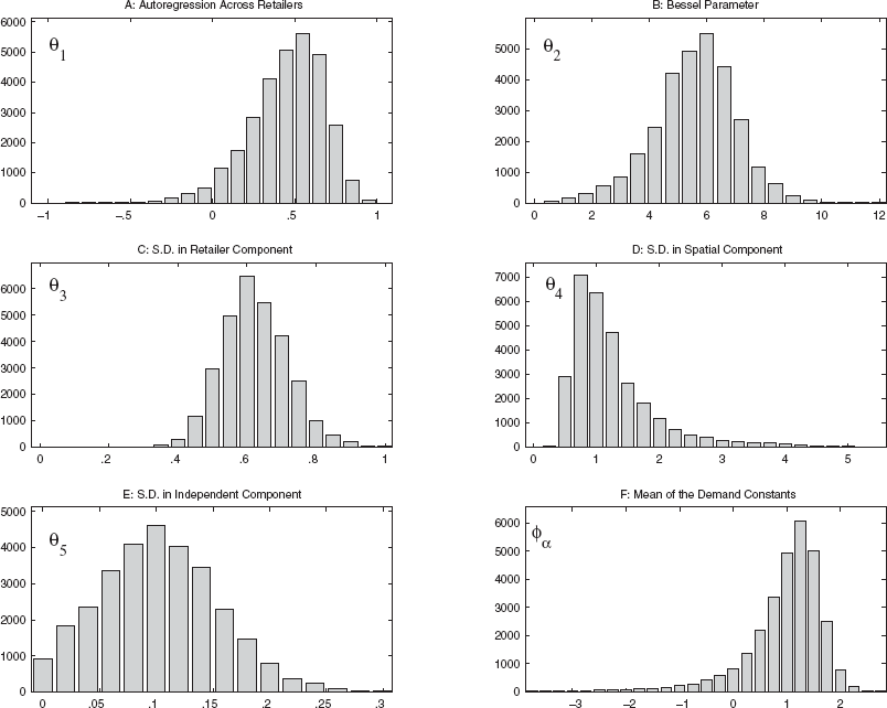
Posterior Distributions for the Parameters of the Cross-Sectional Model For α

The retailer autoregression parameter, θ_α1, has a mode at approximately .5, and more than 95% of its probability mass is in positive territory. Therefore, with some degree of confidence, we conclude that the interaction of retailers—net of other spatial influences—is one of local imitation. This may be of some importance to brand managers, because it suggests that the influence of any given retailer extends beyond its own retail territory. For example, without retailer autoregression (i.e., with θ_α1 = 0), the average area over which there is retailer-based spatial correlation of at least .2 has a radius of 240 miles. However, if θ_α1 = .3, then on average, the same level of spatial correlation extends to an area with a 320-mile radius. As θ_α1 increases, so will the area in which retailer-based spatial correlation is at least .2. We note that because of the structure of the retail industry, these patterns of spatial correlation are highly anisotropic.

The distribution of the distance-based covariation parameters provides additional insights into the covariation patterns. The Bessel parameter θ_α2 has a mean of approximately 5.5 (for an interpretation, see the top graph in Figure 1). This means that from a purely distance-based perspective, the demand constants are positively correlated (locally similar) over a long range of distances. However, as we move even farther away (roughly 1600 miles, e.g., Los Angeles, Calif., to Saint Louis, Mo.), the correlation becomes negative. This result is consistent with the data (sales velocity data for Pace Salsa tend to be above the U.S. mean on the West Coast and below the U.S. mean on the East Coast).

A final aspect of the demand constant parameters involves the large right tail of the posterior distribution for θ_α4 (the standard deviation in the spatial component) and the large left tail of the posterior distribution for φ_α (the mean of the demand constants). There are two reasons for these long tails.

First, precise estimates of φ_α are difficult to obtain because of the predominantly positive correlation across space. The impact of strong spatial correlations on the estimation of φ_α can be observed as follows: If we knew the spatial covariance structure, Λ_α, and if we had observed the constants α, ${\hat{φ}}_{α}$ would be the usual generalized least squares estimate with variance ${(ι^{'} Λ_{α^{- 1}} ι)}^{- 1}$ , where ι is an N × 1 vector of ones. The question now is, “Why is this variance large with positive spatial dependence?” Suppose, for ease of exposition, that the diagonal of the covariance matrix contains equal elements. Factoring out the diagonal, we obtain $σ_{α}^{2} {(ι^{'} Γ_{α^{- 1}} ι)}^{- 1}$ as the sampling variance of ${\hat{φ}}_{α}$ , where Γ_α is the correlation matrix and $σ_{α}^{2}$ is the corresponding scale. The term $(ι^{'} Γ_{α^{- 1}} ι)$ is known in the decision sciences as the Clemen–Winkler measure (Clemen and Winkler 1985) and expresses the number of independent observations contained in N dependent observations. Write this number as N′. This number will become very low as the spatial dependence increases. In the specific case of the local demand constants, α_i, for the Pace brand, this number is approximately ten. This means that our 64 spatially dependent demand constants are “worth” only ten independent observations. It is this lack of independent observations that underlies the large posterior variance in the φs.

Second, the lower the draw of the mean, the higher is the likely corresponding draw of the variance conditional on that mean. Because of this correlation, the variance of the posterior distribution of θ_α4 will also be large.

The Spatial Structure of the Demand Residuals

Table 2 presents the percentiles and mean for the posterior distribution of θ_η. Because there are NT observations of e_it, these posterior distributions are much tighter than those for the demand constants (for which we only had N observations). Computations on the draws for θ_η suggest that approximately 68% of the cross-sectional variance in the dynamic demand shocks is either retailer related (31%) or distance based (37%), whereas only 32% of the cross-sectional variance in the dynamic demand shocks is independent across markets.

Table 2

Credibility Intervals for Selected Model Parameters

Effect	Parameter	Percentiles and Mean
Effect	Parameter	.025	.050	Mean	.950	.975
Intercepts
Autoregression across retailers	θ_α1	−.066	.043	.450	.765	.807
Bessel function parameter	θ_α2	2.390	3.061	5.593	7.834	8.287
S.D. retailer component	θ_α3	.447	.472	.623	.785	.826
S.D. spatial component	θ_α4	.512	.554	1.322	2.899	3.792
S.D. independent component	θ_α5	.008	.018	.102	.191	.211
Mean intercept	φ_α	−1.732	−.693	1.868	1.812	1.953
Price Elasticities
Autoregression across retailers	θ_β1	−.933	−.864	.082	.729	.807
S.D. retailer component	θ_β2	.401	.542	1.251	1.925	2.051
S.D. independent component	θ_β3	.144	.212	.514	.825	.884
Mean price elasticity	φ_β	−2.323	−2.229	−1.873	−1.540	−1.462
Dynamic Component in Sales Velocity
Autoregression across retailers	θ_η1	.254	.267	.328	.386	.395
Spatial dependence	θ_η2	1.899	1.980	2.414	2.861	2.939
S.D. retailer component	θ_η3	.141	.143	.149	.156	.157
S.D. spatial component	θ_η4	.072	.074	.083	.092	.094
S.D. independent component	θ_η5	.066	.067	.069	.071	.071
Autoregression across time	ρ_y	.684	.687	.703	.719	.722
Dynamic Component in Prices
Autoregression across retailers	θ_ξ1	.004	.018	.088	.155	.168
Spatial dependence	θ_ξ2	.182	.346	1.864	3.179	3.371
S.D. retailer component	θ_ξ3	.038	.038	.040	.042	.042
S.D. spatial component	θ_ξ4	.008	.008	.009	.011	.011
S.D. independent components	θ_ξ5	.018	.018	.019	.019	.020
Autoregression across time	ρ_p	.661	.664	.680	.696	.700

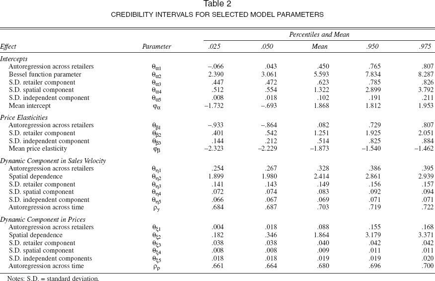
Notes: S.D. = standard deviation.

This spatial dependence of the dynamic demand shocks may indicate that these tend to be common to (multiple co-located) retailers. An example of retailer-based time-varying factors is the effect of unobserved trade promotions to (a geographic segment of) retailers. Although these trade promotions are not directly observed (and may not be observable at all), it is possible to account for their influence through Λ_η.

The spatial dependence in e_t underscores once more that we should expect significant efficiency losses if we treat the multimarket data as cross-sectionally independent (see the previous discussion on price elasticities). In the context of prediction, this result also suggests that local residuals will be informative about the residuals in other nearby markets, even after we account for price effects.

The Spatial Structure of the Price Residuals

Table 2 also presents the posterior distributions for θ_ξ. These suggest that for the dynamic effects in prices, similar results hold as for the demand residuals. The retailer component in cross-sectional covariation of dynamic price shocks is larger than the distance-based component, as would be expected if prices are set at the account level.

Predictions

In this section, we present and analyze the prediction results for demand and price elasticities. We predict these variables for a regularly spaced grid of locations, constructed using a spatial resolution of .02 rads (approximately 80 miles) and spanning the entire continental United States. Predictions in this section are for the last time period of our data set (T_pred = 104).

We evaluate demand predictions using the units in which the model is estimated, as explained previously. Therefore, in Figure 3, we present prediction results for the log of sales velocities. Figure 3, Panel A, shows the posterior means of the predictive distribution at each prediction location. From this graph, we can observe that sales velocities differ greatly across the various regions in the United States. This spatial variation is surprising for a product category (Mexican salsa) with limited or no degree of product differentiation (at least among the nationally available brands). The terraced appearance of the prediction surface, especially in the West, reflects the DMA structure of the data. These plateaus are not completely flat but slightly curved. This is a consequence of the concurrent presence of the distance-based variance component in the model.

Figure 3

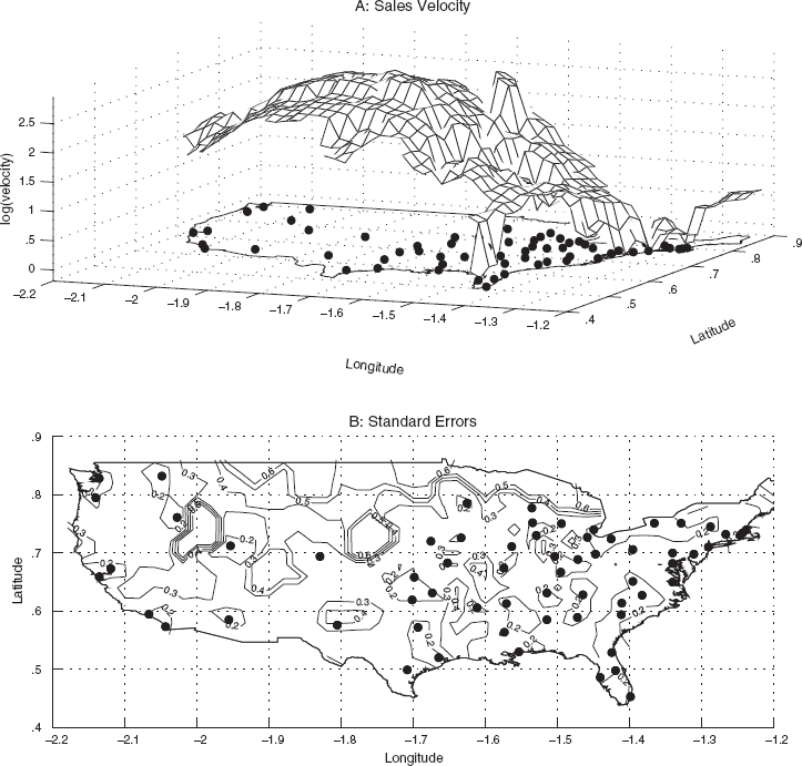
Predictions of Sales Velocity of Pace Salsa in the United States

Figure 3, Panel B, shows the standard errors of the predictions. From this graph, we observe that the standard errors of the predictive distribution have the intuitively correct pattern: Prediction variance is higher for prediction locations farther away from sample points. This is exactly the same as in temporal predictions: The longer the prediction horizon, the larger is the prediction error.

Figure 4 details the predictions for price elasticities. Figure 4, Panel A, presents the predictions of price elasticities. Figure 4, Panel B, presents the standard errors in these predictions. Price elasticities tend to become more pronounced going west. For example, the price elasticity in the westernmost states averages −1.94, whereas in the easternmost states it averages −1.42. Also, the procedure predicts that in almost all locations, price effects are significant. We believe that this is a strong point of the analysis.

Figure 4

Predictions of Price Elasticities of Pace Salsa in the United States

Out-of-Sample Validation

We establish the predictive power of the proposed kriging method using out-of-sample tests. Because our application is spatial, we generated four different types of holdout samples: (1) random removal of IRI markets from our original sample, (2) removal of IRI markets contained in a circle with a random center and a given radius, (3) removal of IRI markets contained in an East–West band with a random location and fixed width, and (4) removal of the IRI markets contained in a North–South band with a random location and fixed width. For each sample pattern, we used three different sample-generation values. For example, we removed 10, 15, and 20 markets from the 64 IRI sample points, and we removed markets located in randomly positioned circles with a radius of .05, .10, and .15 rads (for other values, see Table 3).

Table 3

Mean Squared Error in 100 Randomly Generated Holdout Samples for Pace Salsa (Log of Sales Velocity)

Holdout Generation	Kriging Methods					Naive Methods				Mean Holdout
Holdout Generation	DIRECT	FULL	FULL (θ₁ = 0)	FULL (θ₃ = 0)	KPRICE	NEAR3	NEAR1	AVER	APRICE	Mean Holdout
Random
(number of cities)
(10)	.166	.158	.159	.229	.153	.181	.205	.949	.963	10.00
(15)	.163	.155	.161	.224	.149	.183	.212	.937	.950	15.00
(20)	.194	.185	.193	.255	.179	.213	.236	.974	.988	20.00
Circle
(radius in rads)
(.05)	.207	.187	.186	.268	.182	.245	.338	1.003	1.015	3.25
(.10)	.262	.243	.264	.318	.238	.358	.447	1.123	1.134	8.54
(.15)	.253	.236	.250	.310	.230	.477	.582	1.342	1.351	17.28
East–West
(width in rads)
(.05)	.196	.200	.166	.206	.194	.173	.245	.975	.985	11.45
(.10)	.268	.349	.267	.352	.243	.308	.379	1.175	1.184	20.88
(.15)	.366	.337	.393	.467	.332	.437	.446	1.236	1.245	29.94
North–South
(width in rads)
(.05)	.203	.188	.188	.267	.183	.265	.308	.973	.984	5.50
(.10)	.250	.232	.232	.293	.228	.397	.442	1.200	1.211	9.51
(.15)	.283	.270	.262	.299	.265	.455	.555	1.134	1.146	14.45
Means	.234	.220	.227	.291	.215	.308	.366	1.085	1.096
Percentage difference	−9%	−2%	−6%	−35%	0%	−43%	−71%	−405%	−411%

It is computationally not feasible to generate many holdout samples and then execute an MCMC approach for each of these. In addition, we believe that there is more value in establishing the approximate predictive accuracy of the spatial interpolation method for many different types of holdout samples than there is in knowing the exact predictive accuracy for one or two of these. Therefore, we estimate the approximate accuracy of the kriging predictor by setting the covariance parameters, θ, to reasonable values. This amounts to using a classic kriging predictor with exogenous θ. We chose two sets of parameters for the θs. The first is simply the mean of the posteriors reported in Table 2. The second set of parameters used was intentionally set away from the corresponding posterior means or modes. We did this to prevent the influence of “hindsight wisdom.”

We evaluated three distinct prediction models. In the first model, DIRECT, we use a kriging predictor directly on the log of sales velocity, without price effects. In this model, we directly use Equation 10 to compute ŷ_jt|{y_it} for some location j that is in the holdout sample and all locations i that are in the estimation sample. The second model, FULL, uses the full hierarchical model (see also the subsequent discussion). The third and fourth models are identical to FULL, except that we suppressed retailer interaction (θ₁ = 0) and retailer structure (θ₃ = 0), respectively.⁶ The fifth model, KPRICE, is the same as FULL but assumes that prices in the holdout markets are known.

For an idea of the approximate location of the θ parameters in these various spatial models, we conducted additional MCMC analyses for the DIRECT model and the FULL model with parameter restrictions on θ₁ and θ₃.

The prediction procedure for the most general case of the FULL model works as follows: For each in-sample location, we obtain EGLS estimates of the unobserved spatial variables α and β and compute the residuals e_t and v_t, t = 1, …, T. We then predict for an out-of-sample location j, ${\hat{α}}_{j} | \hat{α}$ , and ${\hat{β}}_{j} | \hat{β}$ using Equation 10 and ê_jt|ê_t and ${\hat{v}}_{jt} | {\hat{v}}_{t}$ using Equation 12. Then we predict y_jt with ${\hat{y}}_{jt} = {\hat{α}}_{j} + {\hat{β}}_{j} {\hat{v}}_{jt} + {\hat{e}}_{jt}$ . Finally, we compute the mean squared error of prediction as the mean of (ŷ_jt − y_jt)² over all j and all t.

We also evaluate four naive prediction models to serve as benchmarks. The first model, NEAR3, predicts sales velocity for holdout locations by averaging over the observations of the nearest three neighbors in the estimation sample. The second model, NEAR1, predicts sales velocity using the observation of the nearest neighbor. The third model, AVER, uses the average of the in-sample observations as a prediction for the out-of-sample locations. From Figure 3, we can easily verify that these three naive predictors are not simply easy-to-beat straw men. Finally, the fourth naive model, APRICE, uses the average of the in-sample EGLS estimates of the intercepts and price effects, assuming an AR(1) temporal structure in the data. Then, APRICE uses these averages and the actual price data from the unsampled markets to predict sales velocity. This model makes use of price information of unsampled markets but does not use any spatial structure.

Table 3 reports the average mean squared prediction error (MSE) in log of sales velocity. This table reports the average MSE for each of the six predictors and for each type of holdout sample, computed across 100 randomly drawn holdout samples and across all 104 time periods. The results for both sets of parameters θ are as follows.

First, the FULL model and the KPRICE model are almost equally good in terms of holdout performance. This suggests that using the v_it observed at sample locations, we can accurately predict the price deviations v_jt for out-of-sample locations j.

Second, the more elaborate models FULL and KPRICE consistently beat the DIRECT kriging approach across all types of holdout samples. Although we believe that both the FULL and the KPRICE model represent a more accurate description of the data-generating process, it can be argued that the improvement these models provide over the DIRECT approach is modest. The reason for this result resides in the combined nature of the more elaborate forecasts, which mitigates their superiority in capturing the essence of the data by leading to higher forecast variability and therefore higher MSE.

Third, if we restrict the retailers to be independent, θ₁ = 0, the predictions (measured by the MSE criterion) are 6% worse than those of KPRICE. Next, by setting θ₃ = 0, we make predictions using only the distance-based component of the model. Now the drop in prediction accuracy is 35%. The predictions using only distance-based covariation are not much different from the naive approach that takes the average of the nearest three markets.

Fourth, the overwhelming result in Table 3 is that when taken together, the kriging approaches greatly outperform the naive predictors such as NEAR3 or NEAR1. If we take the MSE of the AVER predictor, a measure of variance in the data,⁷ we find that the out-of-sample performance of the FULL model is more than four times better than might be expected a priori. In addition, the FULL approach is more than 40% better than NEAR3 and more than 70% better than NEAR1. Finally, among all candidates, the AVER and APRICE predictors are the worst predictors. If we focus momentarily on the relative performance of these two predictors, it may come as a surprise that a model that uses price information is worse than the AVER model, which does not use such information to make predictions. However, it should be recalled that to estimate price effects and intercepts, we must assume that these are constant over time. AVER is more flexible because it uses data of period t only and therefore more accurately tracks temporal shifts in sales velocity. We conclude that the predictive accuracy of kriging methods appears to be superior to that of naive methods.

To illustrate further how well the spatial forecasting method works, the actual variance in the log of sales velocities in the data is .92.

Conclusions and Future Research

The spatial dimension in U.S. multimarket data on food categories is likely to be an important source of variation in the sales performance of nationally distributed brands. As such, it constitutes an overlooked aspect of the food retailing business in the marketing literature and has relevant implications for local marketing policies or micromarketing.

In the context of analyzing the cross-sectional or spatial differences in sales performance, we hope this article has contributed in the following three ways: First, it presents a general prediction method for spatial problems. It introduces optimal spatial predictors, operationalizes them in a marketing context, and reports their performance. The formal prediction methods developed and operationalized here outperform naive methods of spatial prediction on holdout samples.

Second, the article proposes a random effects model of the U.S. retailing industry that may be useful in accounting for unobserved retailer effects in multimarket data. This model captures aspects of both structure and conduct of the retailers in the fast-moving consumer goods industry.

Third, and relatedly, the article develops a feasible way to take into account both the temporal and the spatial nature of the data in the estimation of local marketing-mix effects. Therefore, we can (1) account for unobserved effects with a spatial structure and (2) use the results of neighboring markets to improve the estimates for markets in which information is poor. As a consequence of taking spatial dependencies into account, we obtain more efficient estimates of the price elasticities in local U.S. markets. To the extent that including the spatial dimension of the data helps eliminate model misspecification, we also believe that our estimates are more reasonable.

In terms of future research, spatial analysis can perhaps be used to study retailer power by investigating the cross-sectional properties of undifferentiated product-markets across differentiated retail territories. This methodology is different from that employed in the work of Messinger and Narasimhan (1995) and Lai and Narasimhan (1996), who use historical and game-theoretic methodologies in assessing retailer power.

Through its operationalization of the retailer structure and conduct, this research also opens a new avenue for scientific inquiry into the spatial implications of new product introductions. For example, given the location of retailers, which is truly exogenous for any given product introduction, the choice for lead markets could be guided by a targeting of the markets that are central in the “retail” network, that is, from which most spatial contagion emanates. To evaluate the effectiveness of these efforts, general models of growth across both time and space need to be developed in marketing. Future research projects could deal with these topics.

Footnotes

Some Results for the Prediction Steps

For the prediction of the random components e_jt (and v_jt), where j = N + 1, …, N + M and t = 1, …, T, we need to show that the only observations in e and v that matter for the spatial prediction are e_t = [e_1t … e_Nt]′ and v_t = [v_1t … v_Nt]′, respectively. It is convenient to use the convention that j′ = j − N. We recall that the cross sectional structure contains the following submatrices:

Assuming ergodicity and expanding the AR(1) structure, (A2)

\begin{matrix} E (e_{jt} e_{it - r}) & = & E [\sum_{s = 0}^{\infty} ρ_{y}^{s} η_{jt - s} \sum_{s = 0}^{\infty} ρ_{y}^{s} η_{it - r - s}] \\ = & E [ρ_{y}^{r} \sum_{s = 0}^{\infty} ρ_{y}^{s} η_{jt - r - s} \sum_{s = 0}^{\infty} ρ_{y}^{s} η_{it - r - s}] \\ = & E [ρ_{y}^{s} \sum_{s = 0}^{\infty} ρ_{y}^{2s} η_{jt - r - s} η_{it - r - s}] \\ = & \frac{ρ_{y}^{s}}{1 - ρ_{y}^{s}} Λ_{ηij}, \end{matrix}

where Λ_ηij is the covariation between η_jt and η_it. This implies that the covariation between e_jt and the 1 × N vector e′_t–r of stochastic components at sampled markets at t − r is (A3)

\begin{matrix} E (e_{jt} e^{'}_{t - r}) \underset{(1 \times N)}{=} & \frac{ρ_{y}^{r}}{1 - ρ_{y}^{2}} \end{matrix} Λ_{ηij'}^{21},

where

Λ_{η j'}^{21}

is the j′th row of Λ_η²¹ and is equal to the covariation between the scalar η_jt and the 1 × N vector η′_t of transient spatial effects at the sampled markets and time t. This finally implies that the covariation between e_jt and e′ is equal to the 1 × NT vector

Ψ_{yt} \otimes Λ_{ηj'}^{21}

, where Ψ_yt is the tth row of Ψ_y. Now it is simple to prove (see, e.g., Searle, Casella, and McCulloch 1992) that

Similarly, (A5)

\begin{matrix} V (e_{jt} | e, Ψ_{y}, Λ_{η}) \\ = V (e_{jt}) - (Ψ_{yt} \otimes Λ_{ηj'}^{21}) [Ψ_{y}^{- 1} \otimes {(Λ_{ηj}^{11})}^{- 1}] {(Ψ_{yt} \otimes Λ_{ηj'}^{12})}^{'} \\ = \frac{1}{1 - p_{y}^{2}} Λ_{ηj' j'}^{22} + Ψ_{yt} Ψ_{y}^{- 1} Ψ^{'}_{yt} \otimes Λ_{ηj'}^{21} {(Λ_{η}^{11})}^{- 1} Λ_{ηj'}^{12} \\ = \frac{1}{1 - p_{y}^{2}} [Λ_{ηj' j'}^{22} + Λ_{ηj'}^{21} {(Λ_{η}^{11})}^{- 1} Λ_{ηj'}^{12}], \end{matrix}

where

Λ_{η j'j'}^{22}

is the jth element on the diagonal of the full (M + N) × (M + N) matrix Λ_η. Given these results, the distribution of [e_jt|e,Ψ_y,Λ_η] does not depend on stochastic components other than e_t, and therefore, even for very large T and N, these computations can be done efficiently.

Priors and Full Conditional Distributions

To use the Gibbs sampler, we derived the distributions of all model parameters conditional on the data at the N sampled locations and on the remaining parameters. Because all cross-sectional processes are of size N, during this inference phase of the analysis, we write the N × N submatrix Λ_α¹¹ in Equation 9 as Λ_α. Similarly Λ_β¹¹ will be represented by Λ_β, and so forth.

The MCMC Algorithm

At any stage of the sampler, the conditioning is updated with the most recent draws of the variables in the list of conditionals. We can cross-sectionally vectorize all steps in the algorithm. Again all cross-sectional processes are of size N. Therefore, we again write the N × N leading submatrices Λ_(·)¹¹ as Λ_(·) (for further details, see Appendix B). For each iteration r of the sampler,

References

Boatwright

Peter

, McCulloch

Robert

, and Rossi

Peter

(1999), “Account-Level Modeling for Trade Promotion: An Application of a Constrained Parameter Hierarchical Model,” Journal of the American Statistical Association, 94(December), 1063–1073.

Christakos

George

(1984), “On the Problem of Permissible Covariance and Variogram Models,” Water Resources Research, 20(2), 251–65.

Clemen

Robert T.

, and Winkler

Robert L.

(1985), “Limits in the Precision and Value of Information from Dependent Sources,” Operations Research, 33(2), 427–42.

Cressie

Nodel

(1993), Statistics for Spatial Data. New York: John Wiley & Sons.

Gelman

Andrew

, Carlin

John B.

, Stern

Hal S.

, and Rubin

Donald B.

(1995), Bayesian Data Analysis. New York: Chapman and Hall.

Hoch

Stephen J.

, Kim

Byung-Do

, Montgomery

Alan L.

, and Rossi

Peter E.

(1995), “Determinants of Store-Level Price Elasticity,” Journal of Marketing Research, 32(February), 17–29.

Journel

A.G.

, and Huijbregts

C.J.

(1978), Mining Geostatistics. New York: Academic Press.

Judge

George G.

, Griffiths

W.E.

, Carter Hill

, Lütkepohl

Helmut

, and Lee

Tsoung-Chao

(1985), The Theory and Practice of Econometrics, 2d ed. New York: John Wiley & Sons.

Lal

Rajiv

, and Narasimhan

Chakravarti

(1996), “The Inverse Relation Between Manufacturer and Retailer Margins: A Theory,” Marketing Science, 15(2), 132–51.

10.

Mantoglou

Aristotelis

, and Wilson

John L.

(1982), “The Turning Bands Method for Simulation of Random Fields Using Line Generation by a Spectral Method,” Water Resources Research, 18(5), 1379–94.

11.

Matern

Bertil

(1986), Spatial Variation, 2d ed., Lecture notes in Statistics. New York: Springer-Verlag.

12.

Messinger

Paul R.

, and Narasimhan

Chakravarti

(1995), “Has Power Shifted in the Grocery Channel?” Marketing Science, 14(2), 189–223.

13.

Searle

Shayle R.

, Casella

George

, and McCulloch

Charles E.

(1992), Variance Components. New York: John Wiley & Sons.

14.

Steenburgh

T.J.

, Ainslie

, and Engebretson

P.H.

(2001), “Unleashing the Information in Zip-Codes: Bayesian Methodologies for Massively Categorical Variables in Direct Marketing,” working paper, Johnson School of Management, Cornell University.

15.

U.S. Census Bureau (1994), County and City Data Book. Washington, DC: U.S. Census Bureau.

16.

Vecchia

Aldo V.

(1988), “Estimation and Model Identification for Continuous Spatial Processes,” Journal of the Royal Statistical Society, B, 50(2), 297–312.

17.

Whittle

(1954), “On Stationary Processes in the Plane,” Biometrika, 41(3/4), 434–49.

Using Multimarket Data to Predict Brand Performance in Markets for Which No or Poor Data Exist

Abstract

Multimarket Data

Temporal and Spatial Components in Multimarket Data

Applications of Spatial Analysis to Marketing

Modeling and Prediction Approach

A Model of Market-by-Time Panel Data

Spatial Processes

Spatial Prediction or Kriging

Case 1: Prediction of the Demand Constants αj* and the Price Elasticities βj*

Case 2: Prediction of the Stochastic Terms ejt* and vjt*

Some Differences with the Classic Kriging Predictor

Specific Models of Covariation

Components of the Covariance Structure

Distance-Based Model of Covariation

Retailer Model of Covariation

Covariation Patterns

Empirical Analysis

Data

Estimation

Operationalizations and Model Testing

Functional Form

The Between-Market Model for Intercepts

The Between-Market Model for Price Responses

The Models for the Spatiotemporal Components in the Data

Results

Inferences about Price Elasticities

The Spatial Variance Structures

The Spatial Structure of the Demand Constants

The Spatial Structure of the Demand Residuals

The Spatial Structure of the Price Residuals

Predictions

Out-of-Sample Validation

Conclusions and Future Research

Footnotes

Some Results for the Prediction Steps

Priors and Full Conditional Distributions

The MCMC Algorithm

References

Case 1: Prediction of the Demand Constants α_j* and the Price Elasticities β_j*

Case 2: Prediction of the Stochastic Terms e_jt* and v_jt*