Extending Discrete Choice Models to Incorporate Attitudinal and Other Latent Variables

Abstract

One of the nagging issues in using discrete choice models is how softer attributes, such as attitudes and perceptions, that are not explicitly manipulated within the context of the choice experiment can be accommodated. In many cases, it is reasonable to expect that the choice of a particular alternative may be influenced by non–product-related attributes. For example, latent attitudes and perceptions may play as much of a role in shaping choice as the attributes that have been manipulated and used to define the alternative offerings. In this article, the authors present several full information models that can accommodate latent variables such as attitudes and satisfaction within the context of binary and multinomial choice models. The models proposed are particularly useful when the focus is on understanding how softer attributes can influence choice decisions. The authors accomplish this by integrating structural equation models within the basic framework of binary and multinomial choice models. Two empirical applications are provided. In addition to illustrating the proposed models, these applications provide insights into the circumstances under which the simultaneous factor–choice modeling approach makes a difference.

Choice models have proved to be of enormous value in a wide variety of theoretical and applied settings. Many of the advances in understanding purchase dynamics through the analysis of scanner and panel data, for example, can be traced to the creative use of various binary and multinomial choice models (Erdem and Winer 1999). Similarly, binary and multinomial choice models have been used widely in the experimental analysis of choice (Carson et al. 1994). Experimental choice models have grown in popularity and today are also used in customer satisfaction studies, along with the traditional areas of price and product experimentation. The appeal of this genre of models can be traced to at least two primary features: (1) realism: In real markets, consumers are faced with competing offerings and must choose among them, and (2) experimental control: By varying the levels of an attribute, researchers can estimate how the frequency with which a particular option is chosen varies with changes in the levels of a given attribute, even for attributes that lack sufficient variation in the marketplace.

This article focuses on one of the nagging issues in using discrete choice models in practice; namely, How can softer attributes, such as attitudes and perceptions, that are not explicitly manipulated within the context of the choice experiment be accommodated? In many cases, it is reasonable to expect that the choice of a particular alternative may be influenced by non–product-related attributes.¹ That is, latent attitudes and perceptions may play as much of a role in shaping choice as the attributes that have been manipulated and used to define the alternative offerings. For example, consider the following problem setting, which is, in spirit, similar to one of the empirical applications discussed in a subsequent section:

Although we motivate our work in response to the need to include non-product-related attributes, the large number of product-related attributes that might need to be considered could necessitate that a subset be evaluated (e.g., rated) outside of the experiment. The models to be presented would also prove useful in such cases. We return to this potential application area in a subsequent section.

A cable television provider was interested in assessing the price sensitivity of its current customers to a competitive offer. A sample of customers agreed to participate in an experiment that varied the basic service and the price levels offered by a potential competitor. Respondents were exposed to four different price levels; one price level was equal to their current price structure, whereas the other three offered price savings. After exposure to each price structure, the respondents were asked to indicate on a scale of 0–10 the likelihood of switching to the competitive provider. Among other things, respondents were also asked a series of questions that attempted to assess attitudes toward and satisfaction with their current provider. Satisfaction with the current provider was thought to be particularly important, because the cable industry historically has suffered from low levels of customer satisfaction.

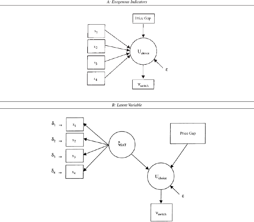
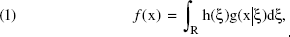
Figure 1 provides a diagrammatic representation of two analysis approaches. The elements in the figure represent the following: There are four reflective indicators of overall satisfaction with the current provider, x₁, x₂, x₃, and x₄; one price variable, price gap, which reflects the savings offered by the competing provider; and one response measure, v_switch, which captures the respondents' likelihood of switching to a competitive provider. The utility of switching is denoted by U_choice, which determines the individual's switching decision as evidenced by v_switch. In Figure 1, Panel A, the utility of switching, U_choice, is directly influenced by the four exogenous manifest variables, x₁, x₂, x₃, and x₄, and the price variable, price gap. In such a case, the four manifest variables would be treated as elements of the deterministic component of utility. The situation in Figure 1, Panel B, is very different. Here, the utility of switching from the current provider, U_choice, is conceptualized as being influenced by a latent satisfaction variable (ξ_SAT) and by the price gap offered, price gap. Although it is straightforward to include individual-specific covariates in the systematic component of utility, incorporating latent constructs such as attitudes and satisfaction is not so easy because the distribution of the latent variable is needed; in other words, the model shown in Figure 1, Panel B, requires use of full information estimation methods.²

Apparently, McFadden (1986) was the first to argue for the need to incorporate latent variables in discrete choice models. And following McFadden's suggestion, Ben-Akiva and colleagues (1998) present various restricted versions of the general models described in this article.

Figure 1

Alternative Representations

More often than not, latent variables have been incorporated into discrete choice models in one of two ways. One way is consistent with the model form shown in Figure 1, Panel A. The reflective indicators (i.e., manifest items) are treated as explanatory predictors of choice (Koppelman and Hauser 1979). The other way is to adopt a two-stage limited information approach in which factor scores on the latent variables are first computed and then entered as error-free explanatory predictors when the multinomial choice model is estimated (Madanat, Yang, and Yen 1995). Unfortunately, both approaches lead to inconsistent and biased estimators. Incorporating the manifest items as (error-free) explanatory predictors of choice ignores the fact that the items contain measurement error, whereas the two-stage approach does not take explicit account of the covariation between the manifest items and choice. Under either approach, the choice model parameter estimates associated with the latent variable or its reflective indicators can be badly misleading.

In light of the difficulty of incorporating latent variables within the discrete choice modeling framework, it is not surprising that constructs such as attitudes and satisfaction have not been used widely in binary and multinomial choice models, and it is doubtful that the potential influence of such constructs on choice could be accurately measured through the simplified methods described previously. Therefore, it is important to develop and investigate the performance of full information estimation techniques that can extend choice models to incorporate latent variables. In the remainder of this article, we present several full information models that can accommodate latent variables such as attitudes and satisfaction within the context of binary and multinomial choice models. The models proposed are particularly useful when the focus is on understanding how softer attributes can influence choice decisions. We accomplish this by integrating confirmatory factor measurement models within the basic framework of binary and multinomial choice models.

We begin by presenting a general form of the basic model. We next present two model extensions that may also prove useful to marketing practitioners and analysts who are investigating unobserved individual differences in the context of the experimental analysis of choice. We provide two empirical applications. In addition to illustrating the proposed models, these applications provide insights into the circumstances under which the simultaneous factor-choice modeling approach makes a difference.

The General Model

Again, let ξ denote the vector of latent exogenous variables with manifest indicators denoted by x. Because only the xs can be observed, any inference must be based on the joint distribution whose density can be written generally as

f (x) = \int_{R} h (ξ) g (x | ξ) dξ,

(1)

where ∫_R is the range space of ξ. The mapping of observed items to the latent factors is accomplished by the following measurement equations:

x_{j} = α_{j} + λ_{jh} ξ_{h} + δ_{j} for j = 1, 2, \dots, p,

(2)

where x_j is a random vector of observed scores for item j, α_j is a measurement intercept for item j, λ_h is a factor loading that maps item j on to latent factor h, and ξ_h and δ_j are latent factors and errors, respectively, which are, as usual, assumed to be uncorrected. Note, finally, that because the scale of the latent variable is arbitrary, we set α_j = 0 and E(ξ_h) = κ = 0 ∀j,h.

There are two important features of Equation 2 that warrant mention. The first is that the ξ_s affect only the mean of the conditional distribution of the xs; that is,

g (x | ξ) \sim D_{p} (α + λξ, Ψ),

where D denotes a specific distributional assumption—for example, normal—and Ψ = Cov(δ,δ′). The second feature is that the conditional mean of x is a linear function of the ξ_s; that is,

E (x | ξ) = α + λξ .

As is customary, we assume that ξ ˜ N_p(0,I), which we use in computing the unconditional density of x as shown in Equation 1.

Consider now, for any particular individual, a discrete choice model of the following form:³

It suffices to denote that particular respondents have been omitted for notational simplicity.

U_{i} = z_{i} β + ξ_{i} γ + ε_{i},

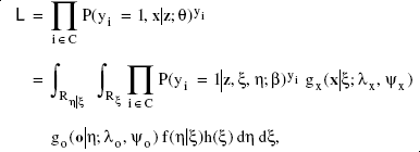
where U_i denotes the utility of alternative i, z_i is a (1 × k) vector of attributes (i.e., explanatory variables) describing alternative i, β is a (k × 1) vector of fixed coefficients reflecting the importance of an attribute on the utility of an alternative, ξ_i is a (1 × h) vector of latent variables scores for alternative i, γ is a (h × 1) vector of fixed coefficients reflecting the importance of each latent factor on the utility of an alternative, and ε_i is an i.i.d. random error component. This formulation implies that the utility of an alternative is a function of unknown latent variables; however, the latent variables are, by definition, not directly observable, and all of the available information is contained in the manifest items. A solution to this problem is first to condition on the latent variables and then to integrate over their joint distribution in evaluations of the utility of an alternative. Denoting the latent variables by ξ as previously and assuming that the error components δ and ε are independent, we can express the joint probability of observing the choice indicator, y_i, and the manifest items as

P (y_{i} = 1, x | z; θ) = \int_{R_{ξ}} P (y_{i} = 1 | z, ξ; β) g (x | ξ; λ, Ψ) h (ξ) dξ,

(3)

where we have added a subscript to R to emphasize that the integration is over the range space of the latent variables; P(y_i = 1|z, ξ; β) is the choice probability conditional on the latent variables ξ, where β again denotes the vector of choice model coefficients and z again denotes (error-free) explanatory variables in the utility function that may influence choice; g(x|ξ) is the conditional distribution of the manifest items x given the latent variables ξ; h(ξ) represents the distribution of ξ; and θ represents the model parameters (λ, β, ψ).

Notice that we have assumed here that, conditional on the latent variables ξ, the choice probability P(y_i = 1|z, ξ; β) and the distribution of the indicators g(x|ξ; λ, ψ) are independent; that is, the joint distribution of the two can be given by the product of the marginals. This assumption of conditional independence is central to most latent variable models that have appeared in marketing literature. Consider, for example, the common factor model that assumes that the indicators are independent conditional on the factors or the latent class model that assumes that, conditional on the latent classes, all other model variables are independent. Notice also that the same assumption can be made with respect to the indicators x; that is, g(x|ξ; λ, ψ) = Π_jg(x_j|ξ; λ, ψ), where the product is carried out over all the indicators.

Model parameters θ can be estimated by means of maximum likelihood procedures. The component of the likelihood function for any particular individual can be written as

\begin{matrix} L & = \prod_{i \in C} P (y_{i} = 1, x | z; θ) y_{i} \\ = \int_{R_{ξ}} \prod_{i \in C} P {(y_{i} = 1 | z,ξ;β)}^{y_{i}} g (x | ξ;λ,ψ) h (ξ) dξ, \end{matrix}

(4)

where C is the choice set of alternatives for that individual, and all other terms are as before. We note, again, from Equation 4 that with full information estimation, we obtain the marginal probability of the observable variables y_i and x by integrating the product of the conditional probability of y_i and x over the joint distribution of the latent variables ξ.

In developing the basic model, we have, for ease of exposition, described the discrete choice utility function as being influenced only by exogenous latent variables ξ_s. This type of model, as well as several multiple-indicator, multiple-cause variants, has been discussed by others; for a summary, see Ben-Akiva and colleagues (1998). It is reasonable, however, to consider the case in which the choice utility function is also influenced by one or more endogenous latent variables, denoted by η, where the ηs are themselves related to the ξ_s through structural equations. With both endogenous and exogenous latent variables, the likelihood function for any particular individual shown in Equation 4 would be rewritten as

\begin{matrix} L & = \prod_{i \in C} P {(y_{i} = 1, x | z; θ)}^{y_{i}} \\ = \int_{R_{η | ξ}} \int_{R_{ξ}} \prod_{i \in C} P {(y_{i} = 1 | z,ξ,η;β)}^{y_{i}} g_{x} (x | {ξ;λ}_{x} {,ψ}_{x}) \\ g_{\circ} (o | {η;λ}_{\circ}, ψ_{\circ}) f (η | ξ) h (ξ) dη dξ, \end{matrix}

where o denotes the vector of observed scores on the endogenous manifest items, and the subscripts x and o are used to distinguish measurement parameters associated with exogenous and endogenous variables, respectively. Notice that the integrand of the likelihood function is a product of the choice expression conditioned on η and ξ; the densities of the indicators of ξ and η conditioned on ξ and η, respectively; the density of η conditional on ξ; and, finally, the density of ξ. This representation is a general form of the basic model. We discuss extensions to this model in subsequent sections.

Estimation

In general, estimation of this class of models requires multidimensional integrals with dimensionality given by the number of latent variables. For problems with three or fewer latent variables (as in the two case studies that follow), numerical integration using quadrature methods is a viable option. With more than three latent variables, estimation can be accomplished by Monte Carlo integration. We provide an overview of both methods here; further details can be found in the references cited.

Numerical Integration

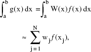
A popular method of computing numerical integrals is to use some form of Gaussian quadrature. The general approach is to use an approximation of the form

\begin{matrix} \int_{a}^{b} g (x) dx = \int_{a}^{b} W (x) f (x) dx \\ \approx \sum_{j=1}^{N} w_{j} f (x_{j}), \end{matrix}

where W(x) is referred to as a weighting function for integrating x, w_j is the quadrature weight, and x_j is the quadrature abscissa. Depending on the particular weighting function chosen and number of points N, it is possible to derive weights and abscissas. Commonly used forms include the Gauss-Legendre, the Gauss-Hermite, and the Gauss-Laguerre. The theory for deriving weights and abscissas for these forms can be found in Press and colleagues (1992).

When the dimension of integration exceeds three, numerical integration methods become impractical. First, the number of function evaluations necessary to evaluate the integral increases exponentially with the increase in the number of dimensions. Second, whereas for a single dimension, the region of integration is defined simply by two numbers (an upper and a lower limit), the shape of a high-dimensional boundary can become extremely complicated.

Monte Carlo Integration

In the case of three or more latent variables, Monte Carlo integration can be used. For example, a simple application of this technique to Equation 4 would involve the following three steps for each observation:

Generate P draws ξ¹, ξ², …, ξ^p from h(ξ).

Evaluate the conditional likelihoods L¹, L², …, L^p at each of these realizations, where Lj (1 ≤ j ≤ P) = Π_i ∊ C^P(y_i = 1|z, ξ; β)y_i g(x|ξ^j; λ, ψ).

Compute the sample average of these conditional likelihoods to get an unbiased estimate⁴ of L; that is, $L = (1 / P) \sum_{j = 1}^{P} Lj$ .

Note that even though the likelihood is unbiased, the log of the likelihood is biased because of the nonlinearity of the transformation.

Various acceleration techniques can be used to reduce the minimum number of draws of ξ required to attain any given accuracy level. For example, antithetic draws involve pairs of draws that are negatively correlated (Davidson and MacKinnon 1993). Draws based on Halton sequences (Train 1999) attempt to achieve uniform coverage over the domain of the mixing distribution h(ξ). Details on estimation methods using simulation can be found in McFadden (1989) and McFadden and Ruud (1994).

We now present two empirical applications, which enable us to illustrate the proposed methodology as well as provide two extensions that would be useful to analysts who suspect either (1) correlated errors or (2) unobserved individual differences. We present each of the two case studies and then provide a general discussion of the likely factors that have contributed to the relative performance of the various models.

Study 1

The data for the first empirical application come from a survey commissioned by a major cable television provider.⁵ Operating in an industry that is about to be deregulated, this company wanted to gain a better understanding of its existing customers as well as investigate the potential for acquiring new customers from competing providers. Among other things, the survey had a section in which a stated preference experiment was conducted. Respondents were asked to assume that in addition to their current provider, they could buy the service from a new entrant. The characteristics of the offer made by the competing company were described—in particular, the new entrant's price structure was varied from the incumbent's price to a situation with a 15% discount, in steps of 5%. For each of the four price points, respondents were asked to indicate their likelihood of switching to the competing offer; responses were collected on a 0–10 likelihood scale.

The identities of the company and industry have been disguised to preserve confidentiality.

To understand the switching decision better, the following additional information was collected: (1) overall satisfaction (sat), (2) overall impression (feeling), and (3) positive word of mouth (wofm). For sat and feeling, the scale ranged from 0 (“highly dissatisfied”) to 10 (“highly satisfied”); for wofm, the scale ranged from 0 (“completely disagree”) to 10 (“completely agree”). Because there are real costs to switching to another provider, the survey also asked respondents a series of questions that focused on possible barriers to switching: (1) the presence of local crews and offices of the other provider (presence), (2) the general level of difficulty in changing providers (hassle), (3) the nature and depth of the relationship with the current provider (relation), (4) the structure of decision making in the household (structure), and (5) the risk associated with a new provider (risk). Responses to each of these items were collected on a 0 (“not at all likely to be a barrier”) to 10 (“highly likely to be a barrier”) scale.

These two sets of items were viewed as having a possible influence on the respondents' likelihood of switching providers. Exploratory and confirmatory factor analysis provided evidence consistent with the view that the first three items represent a latent satisfaction variable (Sat), whereas the next five items reflect a latent cost-of-switching variable (Barriers). With respect to the components of z, in addition to the price discount (discount), two household-specific covariates were also included with a view toward investigating (1) whether households with high cable bills exhibit different switching behavior (cable = natural logarithm of current cable bill) and (2) whether households with a cable modem for Internet access exhibit different switching behavior (modem = 1 if the household has a cable modem, 0 otherwise). Figure 2 depicts the basic model form, and Table 1 shows summary statistics.

Figure 2

Study 1

Table 1

Study 1 Summary Statistics

Models

Limited Information Baseline Models

The first three models rely on limited information estimation and in this sense stand as baseline models. Model M_L1 is a simple ordered probit with no latent variables. The ordered probit model for a 0–10 scale under the assumption of symmetry requires the estimation of five threshold constants. In addition to these five parameters, the model M_L1 estimates four additional parameters: an alternative specific constant β_ASC and β_discount, β_cable, and β_modem, corresponding to the choice covariates (i.e., the elements of z described previously).

Model M_L2 investigates the influence of the satisfaction and barrier variables in addition to the covariates included under model M_L1. Under model M_L2, the eight attitudinal items described previously are used directly in the utility function, without regard for the likely presence of measurement error; therefore, eight additional β-parameters need to be estimated. The final baseline model, M_L3, is consistent with the two-stage limited information approach in which factor scores for the two exogenous latent variables ξ_Sat and ξ_Barriers are included in the utility function as error-free variables. Factor scores were computed by the regression method from a two-factor confirmatory factor model in which the first three attitudinal items loaded on ξ_Sat and the remaining five items loaded on ξ_Barriers.

Full Information Models

Two full information estimation models were also fit. The first model, M_F1, adopts a parameterization consistent with Equation 4. This model estimates four choice parameters, β_ASC, β_discount, β_cable, and β_modem, and two parameters, β_Sat and β_Barriers, that are associated with the two exogenous latent variables. Model M_F1 assumes that the choice data can be adequately characterized by these four choice covariates and the two exogenous latent variables; however, in this study there may be another source of unobserved variation in that respondents were asked to make repeated choices. With repeated choices there can be (within-respondent) choice dependency, which results in correlated errors. This provides the basis for model M_F2, a correlated response model.

The correlated response model is appropriate for situations in which each respondent makes repeated choices (Ben-Akiva et al. 1998; Heckman 1981). Under model M_F2, we hypothesize that the error term ε_in^r, which represents the value taken by ε_i for individual n and response r, can be further decomposed as follows:

ε_{in}^{r} = μ_{in} + υ_{in}^{r},

(5)

where μ_in is an individual and alternative specific error term, and υ_in^r is purely random, that is, independent and identically distributed across alternatives, responses, and respondents. Note that as a direct consequence of this specification, the errors ε_in^r are correlated across responses within respondent n. The specification is completed by defining a distribution for μ_in: A convenient assumption is

μ_{in} \sim N (0, σ_{μ_{i}}^{2})

, where

σ_{μ_{i}}^{2}

is an additional parameter to be estimated. Equivalently, we could set

σ_{μ_{i}}^{2}

to 1 and rewrite Equation 5 as

ε_{in}^{r} = β_{μ_{i}} μ_{in} + υ_{in}^{r},

(6)

where we estimate the coefficient

β_{μ_{i}}

instead of the variance. We hope that by explicitly modeling the residual heterogeneity μ_in, we will obtain improved prediction of the sequences of choices made by the same respondent. Note that our objective with this model is not to model heterogeneity per se but rather to capture correctly the correlation among multiple responses in our survey. We therefore have assumed that the correlation among multiple responses within any respondent is exclusively due to their sharing a common μ and ξ, and we thereby assume that all other slope parameters (β_s) are nonrandom.

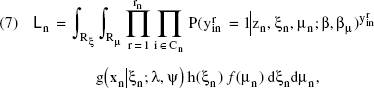
Because the μs, are latent, we first compute the conditional probability of observing a particular sequence of choices from a respondent—in addition to conditioning on the latent variable ξ, we now also must condition on μ. We then derive the marginal probability, as previously, by computing the mathematical expectation of this expression, that is, by integrating over the distribution of ξ and μ. Thus, the likelihood for respondent n can be expressed as

\begin{matrix} L_{n} & = \int_{R_{ξ}} \int_{R_{μ}} \prod_{r = 1}^{r_{n}} \prod_{i \in C_{n}} P {(y_{in}^{r} = 1 | z_{n}, ξ_{n}, μ_{n}; β, β_{μ})}^{y_{in}^{r}} \\ g (x_{n} | ξ_{n}; λ, ψ) h (ξ_{n}) f (μ_{n}) {dξ}_{n} {dμ}_{n}, \end{matrix}

(7)

where y_in^r represents the choice indicator for respondent n, alternative i, and response r; r_n represents the number of responses for respondent n, f(μ_n) denotes the joint distribution of μ_n R_μ is the range of the variables μ, and all other terms are as defined previously. Note that for estimation purposes, we set h(ξ_n) = h(ξ) ∀ n and likewise f(μ_n) = f(μ) ∀ n.

Estimation

Estimation of the limited information baseline models using maximum likelihood is fairly straightforward. The likelihood of observing a rating measured on a 0–10 scale, where 0 implies choice of the incumbent and 1 implies choice of a competing offer for any respondent, can be represented by a symmetric ordered probit of the following form:

\begin{matrix} P (0 | z) & = Φ (- τ_{5} - β^{'} z) \\ P (1 | z) & = Φ (- τ_{4} - β^{'} z) - Φ (- τ_{5} - β^{'} z) \\ ⋮ = ⋮ \\ P (5 | z) & = Φ (- τ_{1} - β^{'} z) - Φ (- τ_{1} - β^{'} z) \\ ⋮ = ⋮ \\ P (10 | z) & = 1 - Φ (- τ_{5} - β^{'} z), \end{matrix}

where τ₁ (1 = 1, 2, …, 5) denotes additional threshold constants to be estimated jointly with the β_s, and Φ denotes the standard normal cumulative distribution. For models M_L1, M_L2, and M_L3, this likelihood function was programmed with the GAUSS statistical software (Aptech Systems 1995) and maximized using standard gradient procedures.

Estimation of the full information models M_F1 and M_F2 is significantly more complicated. Model M_F1 consists of two exogenous latent variables, ξ_Sat and L_Barriers, and M_F2 also contains the individual-specific latent term μ_n. As we mentioned previously, if there are up to three dimensions of integration, quadrature-based numerical methods can be used to evaluate the unconditional likelihood function; accordingly, we used the intquad2 and intquad3 GAUSS procedures to perform the two- and three-dimensional integrations, respectively. Both of these procedures use Gauss-Legendre quadrature (Aptech Systems 1995) and were embedded within the GAUSS maximum likelihood programming environment. We carried out numerical optimization using the Broyden–Fletcher–Goldfarb–Shanno (BFGS) algorithm. In both models M_F1 and M_F2, we specified the conditional choice probability P(y_i = 1|z, ξ; β) as an ordered probit as described previously. Following the arguments presented previously, we assumed the attitudinal indicators to be independent and normally distributed, conditional on ξ_Sat and ξ_Barriers. We assumed ξ_Sat and ξ_Barriers to be bivariate normal with zero means, unit variances, and correlation ϕ_{Sat, Barriers}.

Results

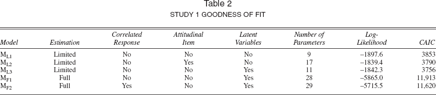
Table 2 provides goodness-of-fit information, and Table 3 provides structural parameter estimates along with asymptotic t-statistics for the baseline and full information models. Model M_L2 provides improved fit over model M_L1 This model estimates eight additional β-parameters associated with the attitudinal indicators, with a log-likelihood of −1839.4, which yields a likelihood-ratio (LR) statistic of 116.3, which with 8 degrees of freedom (d.f.) is highly significant (p < .001). The consistent Akaike information criterion (CAIC) statistic is lower as well.⁶ Model M_L3 also provides a better fit than model M_L1, with respect to both the CAIC and the log-likelihood: LR = 110.6 with 2 d.f. (p < .001). And on the basis of the CAIC, we further conclude that model M_L3 provides a better fit than model M_L2.⁷ With respect to the full information model forms, although the likelihoods obtained under models M_F1 and M_F2 are strictly not comparable, we choose model M_F2 on the basis of the CAIC statistics.

The CAIC (Bozdogan 1987) is defined as −2L_M + Q_M(lnn + 1), where L_M denotes the log-likelihood associated with model M, Q_M is the number of parameters estimated under model M, and n gives the number of observations.

Because models M_L2 and M_L3 are not nested, they cannot be directly compared by means of the LR statistic.

Table 2

Study 1 Goodness of Fit

Model	Estimation	Correlated Response	Attitudinal Item	Latent Variables	Number of Parameters	Log-Likelihood	CAIC
M_L1	Limited	No	No	No	9	–1897.6	3853
M_L2	Limited	No	Yes	No	17	–1839.4	3790
M_L3	Limited	No	No	Yes	11	–1842.3	3756
M_F1	Full	No	No	Yes	28	–5865.0	11,913
M_F2	Full	Yes	No	Yes	29	–5715.5	11,620

Table 3

Study 1 Structural Parameter Estimates^a

Parameter	M_L1	M_L2	M_L3	M_F1	M_F2
β_ASC	−2.1305 (−8.2)	−2.1924 (−8.1)	−2.2091 (−8.4)	−2.2516 (−8.4)	−3.7039 (−5.5)
β_discount	.1914 (25.7)	.2049 (26.7)	.2043 (26.6)	.2097 (26.4)	.3348 (26.6)
β_cable	.0904 (2.5)	.0760 (2.1)	.0798 (2.3)	.0794 (2.2)	.1474 (1.5)
β_modem	−.2209 (−2.1)	−.2902 (−2.7)	−.2658 (−2.6)	−.2717 (−2.6)	−.4804 (−1.4)
β_Sat			−.3169 (−8.4)	−.3896 (−9.4)	−.5625 (−5.3)
β_Barriers			−.0946 (−2.2)	−.1375 (−4.2)	−.1637 (−4.4)
β_μ					1.3156 (14.5)
β_sat		−.0682 (−2.1)
β_feeling		−.0394 (−1.2)
β_wofm		−.0448 (−1.8)
β_presence		−.0215 (−1.6)
β_hassle		.0180 (1.5)
β_relation		−.0290 (−2.0)
β_structure		.0053 (.4)
β_risk		−.0057 (.4)

Asymptotic t-values are shown in parentheses.

In general, there is considerable similarity in the structural parameter estimates obtained under the various model forms. The same is true for the measurement parameter estimates. Table 4 provides measurement parameter estimates for the best fitting baseline model, model M_L3, and the two full information models. All the model forms yield parameter estimates that have the expected algebraic signs, with the exception of model M_L2. Under this model, β_hassle and β_structure have algebraic signs that are contrary to expectations.⁸ In addition, it appears that the attitudinal variables have a relatively minor impact on the decision to stay with the current provider—only two effects, β_sat and β_relation, are statistically significant (one-sided test). Under all model forms, the alternative specific constant parameter β_ASC is negative and indicates that, all else being equal, consumers prefer to stay with their current provider—a measure of the incumbent advantage. The price discount effect β_discount is positive and significant, indicating that price discounts indeed influence the probability of switching providers. The cable usage parameter β_cable is also positive, which suggests that households with high cable bills have a higher propensity to switch, though under model M_F2 this effect is not statistically significant (p > .05). The modem ownership parameter estimate β_modem is negative, in support of the hypothesis that owning a modem makes a household less likely to switch providers (perhaps because of the greater hassle and higher stakes involved), though again, under model M_F2 this effect is not statistically significant.

This will likely be a common problem whenever perceptual and attitudinal indicators are directly included in the utility function, which is another serious limitation of this approach.

Table 4

Study 1 Measurement Parameter Estimates

Parameter	Model M_L3		Model M_F1		Model M_F2
Parameter	Estimate	t-Value^a	Estimate	t-Value^a	Estimate	t-Value^a
λ_{sat, Sat}	1.9347	(18.0)	2.0272	(18.1)	1.9262	(23.8)
λ_{feeling, Sat}	2.0539	(18.7)	2.1260	(18.5)	2.0171	(24.1)
λ_{wofm, Sat}	2.2595	(16.9)	2.4192	(16.4)	2.2984	(20.2)
λ_{presence, Barriers}	2.4410	(11.7)	2.3195	(10.9)	2.3086	(11.0)
λ_{hassle, Barriers}	2.2215	(9.9)	2.2360	(9.9)	2.2479	(10.1)
λ_{relation, Barriers}	2.3291	(11.9)	2.3820	(12.0)	2.3543	(12.0)
λ_{structure, Barriers}	1.6012	(8.6)	1.4096	(7.6)	1.4103	(7.7)
λ_{risk, Barriers}	2.0326	(10.1)	2.0717	(10.1)	2.0554	(10.1)
ψ_sat	.8401	(6.9)	.7868	(13.9)	.7621	(13.1)
ψ_feeling	.7212	(5.7)	.8303	(14.7)	.8156	(14.1)
ψ_wofm	1.7100	(8.4)	2.0147	(17.4)	1.9802	(17.2)
ψ_presence	5.5736	(8.2)	5.8850	(16.6)	5.8438	(16.4)
ψ_hassle	7.5118	(9.3)	7.5408	(18.5)	7.4071	(18.3)
ψ_relation	4.8646	(8.0)	4.6293	(14.9)	4.6656	(15.0)
ψ_structure	5.6218	(9.9)	5.7806	(20.3)	5.9451	(20.2)
ψ_risk	6.0814	(9.3)	6.0629	(18.1)	6.0599	(18.0)
ϕ_{Sat, Barriers}	.3800	(6.0)	.3770	(5.7)	.3599	(5.7)

Asymptotic t-values.

Given the similarity of parameter estimates in this problem setting, the primary advantage of using either of the full information model forms is increased precision. (We discuss the reasons for this further after the second application.) Notice that the parameter estimates associated with the exogenous latent satisfaction and cost of switching constructs, β_Sat and β_Barriers, under both of these models are higher in absolute value and more robust than those obtained under model M_L3, reflecting the disattenuation from measurement error. This is especially true for β_Barriers. Notice finally that β_μ is robust and statistically significant.⁹ This indicates that the choice data cannot be adequately represented unless the dependency resulting from collecting repeated choices from the same respondent is captured.

The uniformly larger structural parameter estimates obtained under model M_F2 compared with M_F1 reflects a scale difference between the two models. The scaling of utility is defined by the normalization of the error term in the utility function, in this case, as a probit. This error variance is smaller for model M_F2 than model M_F1 because the heterogeneity term absorbs some of the variance. Because the scale is inversely related to the error variance, the same normalization in both models results in larger parameter values under model M_F2 than under model M_F1.

Study 2

The data for the second study come from an ongoing customer satisfaction study conducted for a health care provider. This health care provider was facing several challenges. First, satisfaction scores had been falling for the last six quarters, putatively because of several rate increases. Second, the firm, through competitive intelligence and regulatory disclosure, had reliable information that a national underwriter was going to enter two of its larger served markets aggressively, offering plans that might be attractive to the first provider's core policyholders. Given this competitor's historical behavior, management believed that the competitor's plans would likely appeal to the largest segment of policyholders, those with a basic configuration of benefits, who paid approximately $200–$250 per month, by offering a similar benefits package but with more attractive deductibles, copayments, or reimbursement options. Therefore, in the third quarter of 1999, the customer satisfaction survey was augmented with a view toward assessing the resistance of the first provider's core customer base to such a competitive offer. Specifically, a subset of current policyholders was exposed to a possible competitive offering and asked whether the policyholders would stay or leave.

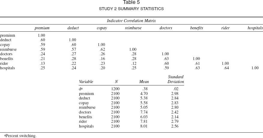
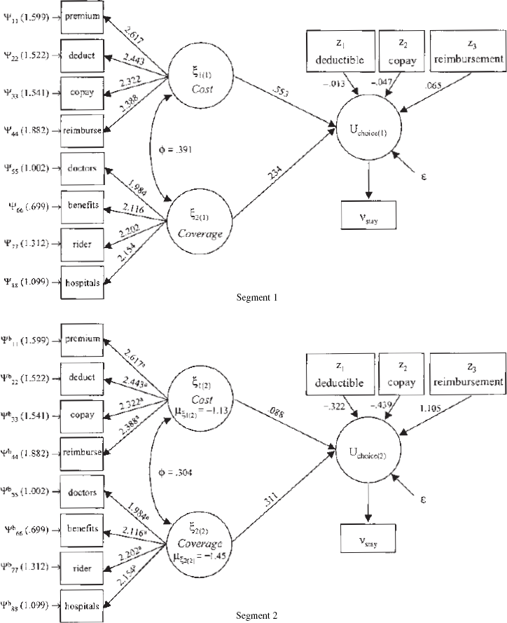
Figure 3 depicts the basic model forms. There are two antecedent exogenous latent satisfaction constructs. The observable indicators for satisfaction with cost (ξ_Cost) are satisfaction with monthly premium (premium), annual deductibles (deduct), amount of copayment (copay), and amount of reimbursement (reimburse). The indicators of satisfaction with coverage ξ_Coverage are quality of doctors in plan (doctors), basic medical care benefits (benefits), extended policy rider coverage (rider), and the quality of the hospitals in the plan (hospitals). Summary statistics are shown in Table 5. The choice manipulation involved offering more attractive offers with regard to mandatory deductibles, copayments, and reimbursement schedules. In response to a favorable change in the amount of deductible (deduct_amt), the amount of copayment (copay_amt), or the percentage reimbursed (reimburse_%), policyholders indicated that they would either stay with their current policy provider or switch policies. Manipulations were randomly assigned to selected policyholders so as to produce a balanced design; that is, over the data collection period, approximately 1/3 of these policyholders were exposed to an offer promising more attractive deductibles, 1/3 were exposed to an offer promising lower copayments, and 1/3 were exposed to an offer promising higher reimbursement levels.

Figure 3

Study 2

Table 5

Study 2 Summary Statistics

Models

Limited Information Baseline Models

As in Study 1, the first three models rely on limited information estimation and stand as baseline models. Model M_L4 is a binary logit (“stay” = 1, “leave” = 0) with no latent variables. In addition to the alternative specific constant, the three covariates, deduct_amt, copay_amt, and reimburse_%, described previously, were included in specifying a policyholder's utility function. Model M_L5 investigated the influence of the eight cost and coverage satisfaction variables in addition to the covariates included under model M_L4. Under model M_L5, the eight attitudinal items described previously are used directly in the utility function, without regard for the likely presence of measurement error. The final baseline model, M_L6, is consistent with the two-stage limited information approach in which factor scores for the two latent variables ξ_Cost and ξ_Coverage are included in the utility function as error-free variables. Factor scores were again computed by the regression method from a two-factor confirmatory factor model in which the first four attitudinal items loaded on ξ_Cost and the remaining four items were restricted to load on ξ_Coverage.

Full Information Models

The first full information model, M_F3, adopts a parameterization consistent with Equation 4. This model estimates all latent exogenous and endogenous parameters simultaneously and assumes that all the choice variation can be adequately captured without the introduction of additional terms. The issue is whether this specification can indeed capture individual choice variation. In Study 1, we introduced the correlated response model for this purpose. However, in Study 2 we do not have replications; each policyholder made only one choice. Therefore, another specification is needed to answer this question, a finite mixture model.

So far, we have assumed that all the choice variation can be entirely explained by the latent variables ξ_s along with any individual or choice covariates specified in z. Finite mixture models have proved useful in capturing unobserved individual differences (Dillon and Kumar 1996). Although finite mixture multinomial choice models and finite mixture confirmatory factor and structural equation models have been developed (see DeSarbo, Ramaswamy, and Cohen 1995; Jedidi, Jagpal, and DeSarbo 1997; Yung 1997, respectively), finite mixture model analogies to Equation 4 have not appeared in the marketing research literature.

Finite mixture models assume that people belong to different segments that are exhaustive and mutually exclusive. Each of the segments s (s = 1, …, S) is characterized by its set of unique measurement model parameters and choice probabilities. The relative size of segment s is denoted by π_s, (0 < π_s ≤ 1 and Σ_sπ_s = 1). With mixing proportion π_s, the probability of observing choice i and indicators x for any particular person belonging to segment s can be written as

P_{s} (y_{i} = 1, x | z, ξ_{s}) = P_{s} (y_{i} = 1 | z {,ξ}_{s}) g_{s} (x {| ξ}_{s}),

(8)

where P_s(y_i = 1|z, ξ_s) and g_s(x|ξ_s) denote the within-segment choice model and within-segment measurement model, respectively, both of which are conditional on the within-segment latent variables denoted by ξ_s. The unconditional probability is then obtained by summing over the latent classes:

P (y_{i} = 1, x | z; θ) = \sum_{s = 1}^{S} π_{s} P_{s} (y_{i} = 1, x | z; θ_{s}) .

(9)

Thus, the likelihood for any one person can be written as

\begin{matrix} L & = \sum_{s=1}^{S} π_{s} \prod_{i \in C} P_{s} {(y_{i} = 1, x | z; θ_{s})}^{y_{i}} \\ = \sum_{s=1}^{S} π_{s} \int_{R_{ξ_{s}}} \prod_{i \in C} P_{s} {(y_{i} = 1 | {z,ξ}_{s}; β)}^{y_{i}} \\ g_{s} (x | ξ_{s}; λ_{s}, ψ_{s}) h (ξ_{s}) {dξ}_{s}, \end{matrix}

(10)

where all terms have been previously defined and the subscript s denotes segment-specific effects.

With respect to the latent variable measurement model, there potentially is a large number of model forms that can be considered. These models come about from relaxing or imposing restrictions on which parameters are free to vary across segments. And, as Blåfield (1980) and Yung (1995) discuss, such restrictions are important from both a substantive and an estimation perspective. From a substantive perspective, for example, if the number of latent variables (i.e., factors) is allowed to vary across segments, then it will always be impossible to compare factor loadings; similarly, if factor loading matrices are allowed to vary across segments, then we must set κ_s = 0, and diag(Φ_s) = I_p, where κ_s denotes the mean of ξ in segment s, for all s ≤ S, in order to make comparisons of the factor loading matrices among the segments. From an estimation perspective, the measurement model is not identified in general form. Normality of the xs ensures that the mixture distribution is identified (Teicher 1963).¹⁰ The identifiability of the factor model depends on the set of restrictions imposed on the mean and covariance structure. For example, if only the factor loadings are set invariant across segments, the conditional mean structure for any segment is generally not identified.¹¹

Unfortunately, the likelihood function in this class of models may be unbounded, and multiple local maxima are possible. However, Titterington, Smith, and Makov (1985) point to many empirical studies and to asymptotic theory, which suggest the existence of satisfactory local maximum.

Yung (1995) provides an informative discussion of other cases of underidentified model specifications in the context of finite mixture confirmatory factor models.

Estimation

Estimation of the limited information baseline models using maximum likelihood is straightforward. With a binary choice indicator, the models considered here treat the conditional probability of choice as an extreme value, thus resulting in a logit, as opposed to an ordered probit as was used in Study 1.

Estimation of the full information models proceeded in much the same manner as in Study 1, with the exception of the logit specification; we used intquad2 and intquad3 to perform the numerical integration within a GAUSS maximum likelihood estimation environment that relied on the BFGS algorithm. For model M_F3, we assumed the attitudinal indicators to be independent and normally distributed, conditional on ξ_Cost and ξ_Coverage. We assumed ξ_Cost and ξ_Coverage to be bivariate normal with zero means, unit variances, and correlation ϕ_Cost,_Coverage. Models M_F3a, M_F3b, and M_F3c represent mixtures with two, three, and four latent segments. For these models, we used a similar estimation method as for model M_F3, except that to ensure identification for each model, we set for the first segment, κ₁ = 0 and diag(Φ₁) = I_p, where I_p is a p × p identity matrix. In addition, we imposed the constraint of invariant error variances, which also aids in identification, and set the measurement intercepts and factor loadings invariant across segments, so that we estimate segment-specific latent variable means, variances, and structural parameters. To further minimize problems of local minima, we used 50 random start values and retained the best fitting model.

Results

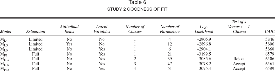
Table 6 provides goodness-of-fit information. Models M_F3a, M_F3b, and M_F3c represent the two–, three–, and four–latent class solutions, respectively. With respect to the “best” baseline model, the results are somewhat inconclusive, though favoring model M_L4. On the basis of the LR statistic, we would conclude that model M_L5 provides an improvement in fit over model M_L4. This model estimates eight additional β-parameters associated with the attitudinal indicators with a log-likelihood of −2896.8, which yields an LR statistic of 18.2, which with 8 d.f. is statistically significant (p < .05). However, the CAIC statistic favors model M_L4. Model M_L6 does not provide improved fit over model M_L4 (LR = 3.6 with 2 d.f.). Therefore, model M_L4 is the preferred model. With respect to the full information models, the finite mixture models M_F3a–M_F3c provide statistically significant improvements in fit over model M_F3, which suggests that substantial choice variation cannot be adequately captured by an aggregate model with only common effects. Furthermore, the goodness-of-fit measures point to the adequacy of the two-segment (S = 2) solution.

Table 6

Study 2 Goodness of Fit

Model	Estimation	Attitudinal Items	Latent Variables	Number of Classes	Number of Parameters	Log-Likelihood	Test of s Versus s + 1 Classes	CAIC
M_L4	Limited	No	No	1	4	–2905.9		5846
M_L5	Limited	Yes	No	1	12	–2896.8		5896
M_L6	Limited	No	Yes	1	6	–2904.1		5860
M_F3	Full	No	Yes	1	21	–3199.5		6579
M_F3a	Full	No	Yes	2	39	–3085.6	Reject	6506
M_F3b	Full	No	Yes	3	47	–3078.2	Accept	6561
M_F3c	Full	No	Yes	4	51	–3075.4	Accept	6589

Structural parameter estimates for the baseline models along with asymptotic t-statistics are provided in Table 7. Again, we find that the baseline model forms yield fairly similar parameter estimates. Notice that the alternative specific constant parameter β_ASC is positive and statistically significant, indicating that, all else being the same, consumers prefer to stay with their current policy provider. The negative parameter estimates for $β_{{deduct}_{amt}}$ and $β_{{copay}_{amt}}$ indicate that policyholders are generally attracted to lower deductibles and lower copayments; however, note that across all three baseline models, these effects are not statistically significant, and as such they do not play an important role in a policyholder's decision to stay or leave. In contrast, the statistically significant and positive parameter $β_{{reimburse}_{%}}$ indicates that, in general, policyholders prefer plans with larger reimbursement schedules, and perhaps more important, competitive policies that offer higher reimbursements will increase the likelihood of attrition. Finally, notice that regardless of how the satisfaction covariates are parameterized, their effects on a policyholder's decision to stay is minimal—neither β_Cost nor β_Coverage is statistically significant under model M_L6, and under model M_L5, none of the statistically significant satisfaction effects has the proper algebraic sign. As we indicated in the context of Study 1, whenever attitudinal items are used directly in the utility function, it is likely that multicollinearity will adversely affect the parameter estimates obtained.

Table 7

Study 2 Structural Parameter Estimates: Baseline Models^a

Parameter	M_L4	M_L5	M_L6
β_ASC	3.5781 (18.9)	3.0326 (16.5)	3.5887 (18.1)
$β_{c o p a y_{a m t}}$	−.0919 (−1.1)	−.1154 (−.7)	−.0645 (−1.2)
$β_{r e i m b u r s e_{%}}$	−.1317 (−1.5)	−.1670 (−1.1)	−.1657 (−1.4)
$β_{d e d u c t_{a m t}}$	.1811 (2.9)	.1202 (1.9)	.1856 (2.0)
β_Cost			.1236 (1.0)
β_Coverage			.1914 (1.4)
β_premium		−.1132 (−2.4)
β_deduct		−.0013 (−.2)
β_copay		.0048 (.4)
β_reimburse		.0555 (.6)
β_doctors		.0780 (1.1)
β_benefits		−.1298 (−2.0)
β_rider		.0953 (.8)
β_hospitals		−.0731 (−.5)

Asymptotic t-values are shown in parentheses.

Structural parameter estimates for models M_F3 and M_F3a are shown in Table 8. Figure 4 shows both measurement and structural parameters for model M_F3a. Notice first that model M_F3 provides a different take on the importance of the latent satisfaction constructs than that suggested by the limited information model forms. Notice also that the parameters associated with both latent satisfaction constructs β_Cost and β_Coverage are statistically significant (p < .01). And finally, the incumbent effect as evidenced in β_ASC is smaller than under any of the limited information model forms.

Figure 4

Study 2: Model M_F3a

Table 8

Study 2 Structural Parameter Estimates: Models M_F3 and M_F3a^a

Parameter	M_F3	M_F3a		Factor Means
Parameter	M_F3	Segment 1	Segment 2	Segment 2
β_ASC	1.6511	3.7783	−1.3443
	(21.4)	(3.3)	(4.2)
$β_{{deduct}_{amt}}$	−.0645	−.0133	−.3222
	(−1.2)	(−.9)	(3.3)
$β_{{copay}_{amt}}$	−.1657	−.0471	−.4387
	(−1.9)	(−.3)	(−2.9)
$β_{{reimburse}_{amt}}$	.1766	.0654	1.1052
	(2.7)	(1.3)	(4.7)
β_Cost	.3896	.5531	.0876	−1.13
	(9.4)	(7.3)	(.5)	(−7.4)
β_Coverage	.2375	.2344	.3111	−1.45
	(4.2)	(3.7)	(2.8)	(−6.9)

Asymptotic t-values are shown in parentheses.

Model M_F3a provides a more complete story regarding the role of satisfaction in a policyholder's decision to stay in the sense that the two latent segments can be viewed as two discrete latent moderators of the relationships among the latent exogenous satisfaction constructs, the choice covariates, and choice. From the mean levels for the satisfaction latent exogenous constructs provided in Table 8 and shown in Figure 4, we find that the latent segments are very different. The mean levels for the latent satisfaction constructs across the segments show that Segment 2 (41.1% of the sample) is a relatively dissatisfied group and has the lowest satisfaction levels. And the mean differences for both latent satisfaction constructs are highly significant across both groups. Low levels of satisfaction produce a group of policyholders that is very likely to leave and that does not endow the incumbent with much equity—notice that β_ASC is negative and statistically significant. Compared with model M_F3, which suggests that both latent satisfaction constructs are significant determinants of the decision to stay with the current policy, model M_F3a points to the presence of both common and segment-specific effects. In Segment 1, representing 58.9% of the policyholders, ξ_Cost and ξ_Coverage satisfaction are the only significant drivers of choice. Segment 1 is, in general, a satisfied group, and satisfaction is the major reason for members staying. Policyholders in Segment 2 have a much higher probability of leaving in response to more advantageous deductible, copayment, and reimbursement offers—notice that $β_{{deduct}_{amt}}$ , $β_{{copay}_{amt}}$ , and $β_{{reimburse}_{%}}$ are all statistically significant (p < .01). As mentioned previously, compared with Segment 1, Segment 2 is a relatively dissatisfied group, and only satisfaction with ξ_Coverage is a determinant of choice. In contrast to limited information model forms, the full information models clearly show that satisfaction indeed matters.

Discussion

The case studies presented in this article raise three important questions: (1) What are the potential implications of the different estimation approaches on marketing decisions? (2) What accounts for the different conclusions regarding the relative performance of full information estimation models? and (3) In what problem settings can this class of models prove useful?

Implications of Different Approaches

The two empirical applications produced very different conclusions regarding the efficacy of using full information estimation techniques when incorporating latent variables into discrete choice models. From a managerial perspective, the substantive differences between the baseline models and the full information model forms in Study 1 were minor, though the full information models yielded more precise estimates. In contrast, in Study 2 the differences were substantial, and the use of any of the baseline models would provide managers with misleading results regarding the role of satisfaction in determining whether to stay with the current policy.

Specifically, managers using the two-stage limited information method would conclude (erroneously) that satisfaction plays a limited role in determining choice of policy, and therefore they might discontinue or underinvest in their customer satisfaction programs. The full information methods, in contrast, clearly illustrate the importance of satisfaction—the finite mixture solution would aver that satisfaction levels with cost and coverage are the primary determinants of choice in almost 60% of the population. Note also that the coefficient of ξ_Coverage is higher than ξ_Cost in the limited information model, which suggests that managers should focus greater attention on improving their subscribers' perceptions of the coverage aspects of their policy as opposed to cost perceptions, that is, by improving the quality of enrolled doctors and hospitals, ensuring basic medical benefits, and improving extended policy rider coverage. The full information models, however, strongly dispute that suggestion. The finite mixture model asserts that ξ_Coverage is more important than ξ_Cost only in one segment of policyholders, which accounts for 40% of the population, and that for 60%, ξ_Cost is more important. Therefore, all else being equal, more marketing resources should be allocated to improving satisfaction with cost aspects to counter the threat from the national underwriter. The limited information models would thus lead managers to two actions that are potentially deleterious: first, an overall underinvestment in their customer satisfaction programs, and second, an inefficient allocation of marketing resources between these two facets of satisfaction.

Relative Performance Issues

To further investigate the relative performance of these models, we conducted a Monte Carlo simulation experiment. Aside from the method of estimation (limited versus full), the simulation experiments focused attention on four factors thought to influence relative model performance: (1) the number of respondents, (2) the number of items per construct, (3) item reliability, and (4) the strength of the structural parameter linking the latent variable to choice. The results of the simulations suggest that full information models will be superior to limited information models, regardless of sample size, when item reliabilities are poor to moderate and when the latent variables explain a substantial amount of the variation in choice. More specifically, the simulation results clearly show that the two estimation approaches differ the most with respect to their ability to capture the structural parameter that links the latent variable and utility. In the presence of a strong relationship between the latent variable and utility, the two-stage limited information approach yielded structural parameters that had biases averaging more than 18%.¹² The root mean square errors associated with the limited information methods were three times larger than with full information estimation. And larger sample sizes did not result in substantially improved parameter recovery for the two-stage limited information approach. As a general rule, full information estimation yielded estimates of the structural parameter that were in most cases at least twice as precise as those obtained with the two-stage limited information approach.¹³

Note again that the biases in the limited information methods arise because the latent constructs are treated as error free instead of as random variables. This is analogous to the bias or attenuation in slope parameters in regression equations in which an independent variable is measured with error (Greene 2000). The full information methods are unbiased.

Specific details on how the sampling experiments were conducted and results can be obtained by contacting the authors.

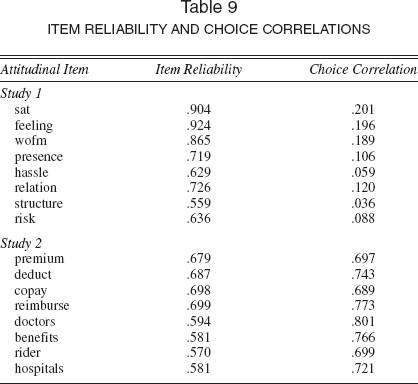
Table 9 provides additional support for the simulation findings in the context of the two empirical studies. For each manifest item, Table 9 gives the item reliabilities and the bivariate correlations with the choice variable. In Study 1, the latent variable indicators were relatively reliable but had weak association with the choice variables. Notice that the reliabilities are fairly robust, especially for the first three attitudinal items that load on ξ_Sat, and the highest choice correlation is approximately .20 (in absolute value). In contrast, in Study 2 the items were for the most part less reliable but had much stronger association with choice. Notice that the weakest choice correlation is .69, which means that the satisfaction items explain a larger percentage of the variation in choice. Therefore, our practical finding from the two case studies would be that the full information methods offer significant improvements over their limited information counterparts when the latent constructs are strong drivers of choice; in the absence of such a relationship, there does not appear to be a substantive difference between the two.

Table 9

Item Reliability and Choice Correlations

Attitudinal Item	Item Reliability	Choice Correlation
Study 1
sat	.904	.201
feeling	.924	.196
wofm	.865	.189
presence	.719	.106
hassle	.629	.059
relation	.726	.120
structure	.559	.036
risk	.636	.088
Study 2
premium	.679	.697
deduct	.687	.743
copay	.698	.689
reimburse	.699	.773
doctors	.594	.801
benefits	.581	.766
rider	.570	.699
hospitals	.581	.721

Application Areas

We perceive at least three general application areas in which the models developed in this article may provide large benefit. The first is in modeling customer satisfaction and its relationship to observed behaviors such as provider choice. The importance of customer retention has been well documented, and many firms have allocated significant dollars to developing or enhancing existing customer satisfaction programs. The full information methods described and illustrated in two empirical applications enable a marketing manager to assess, much more accurately than do existing limited information methods, the efficacy of investments in a customer satisfaction program by accurately predicting its impact on metrics such as attrition, revenues, and profitability.

The second application area is in the modeling of scanner-panel data. It is reasonable to suspect that brand perceptions and consumer attitudes play a major contributing role in what, how much, and when consumers buy. With the models described and illustrated herein, it is possible to augment conventional scanner-panel data with information on potentially important latent constructs that represent the softer brand attributes or consumer attitudes. Consider, for example, the salted snacks category and, in particular, potato chips. A pure scanner-panel attribute–based approach (Fader and Hardie 1996) might consider only independent variables such as brand name (e.g., Frito-Lays, Ruffles), fat content (e.g., regular, reduced fat, fat free), size (e.g., 8 oz., 16 oz.), package type (e.g., bag, canister), flavor (e.g., regular, barbecue, sour cream and onion), and price. However, there are other potentially important softer attributes that could influence a customer's choice of a particular stockkeeping unit. For example, attitudes toward “healthiness” or “natural” ingredients could influence choice. Some consumers could be influenced by the texture and appearance of the chip; others could be influenced by their desire for a chip that is hot or spicy; and still others could be influenced by the communicated positioning of the brand, that is, brand imagery—a “contemporary brand,” a “fun brand,” and so forth. These attributes are not, in a strict sense, directly measurable in terms of a brand's physical attributes but rather, in most cases, must be indirectly measured through psychometric methods. The models presented in this article provide a direct and efficient means of incorporating these perceptual and attitudinal attributes as latent variables in conjunction with harder attributes in predicting stockkeeping unit choice, thus resulting in a richer and more veridical description of consumer behavior.

The third application area is also related to the design and analysis of choice experiments. The primary motivation for the models developed in this article was the need to accommodate non–product-related attributes. However, even with the availability of highly efficient D-optimal designs, there may be cases in which not all of the many product-related attributes can be reasonably considered within the context of the experimental design. The lack of large sample sizes or fears of respondent fatigue or excessive cognitive effort are factors that may lead to the decision to evaluate a subset of product-related attributes outside of the choice experiment. With the use of limited information models, assessing the importance of these attributes would be problematic, especially if they are strong determinants of choice, because structural parameters associated with these covariates would be attenuated. In contrast, estimation with the class of full information models described previously would not suffer in this regard and, in addition to yielding more accurate parameter estimates, would provide a holistic framework for better managing both product-related and non–product-related attribute information.

References

Aptech Systems (1995), GAUSS Command Reference Manual. Maple Valley, WA: Aptech Systems Inc.

Ben-Akiva

, Walker

, Bernardino

A.T.

, Gopinath

D.A.

, Morikawa

, and Polydoropoulou

(1998), “Integration of Choice and Latent Variable Models,” paper presented at the American Marketing Association ART Forum, Keystone, CO (June).

Blåfield

(1980), Clustering of Observations from Finite Mixtures with Structural Information, Jyvaskyla Studies in Computer Science, Economics, and Statistics, 2. Finland: Jyvaskyla University.

Bozdogan

Ham

(1987), “Model Selection and Akaike's Information Criterion (AIC): The General Theory and Its Analytical Extensions,” Psychometrika, 52(September), 345–70.

Carson

Richard T.

, Louviere

Jordan J.

, Anderson

Donald A.

, Arabie

Phipps

, Bunch

David S.

, Hensher

David M.

, Johnson

Richard M.

, Kuhfeld

Warren F.

, Steinberg

Dan

, Swait

Joffre

, Timmermans

Harry

, and Wiley

James B.

(1994), “Experimental Analysis of Choice,” Marketing Letters, 5(4), 351–68.

Davidson

, and MacKinnon

J.G.

(1993), Estimation and Inference in Econometrics. Oxford, UK: Oxford University Press.

DeSarbo

Wayne

, Ramaswamy

Venkat

, and Cohen

Steve

(1995), “Market Segmentation with Choice-Based Conjoint Analysis,” Marketing Letters, 6(2), 137–47.

Dillon

William R.

, and Kumar

(1996), “Latent Structure and Other Mixture Models in Marketing: An Integrative Survey and Review,” in Advanced Methods in Marketing Research, Richard

P. Bagozzi

, ed. Cambridge, MA: Blackwell Publishers, 295–351.

Erdem

Tulin

, and Winer

Russell

(1999), “Econometric Modeling of Competition: A Multi-Category Choice-Based Mapping Approach,” Journal of Econometrics, 89(November), 159–75.

10.

Fader

Peter S.

, and Hardie

Bruce G.S.

(1996), “Modeling Consumer Choice Among SKUs,” Journal of Marketing Research, 33(November), 442–52.

11.

Greene

William H.

(2000), Econometric Analysis. Upper Saddle River, NJ: Prentice Hall.

12.

Heckman

J.J.

(1981), “The Incidental Parameters Problem and the Problem of Initial Conditions in Estimating a Discrete Time-Discrete Data Stochastic Process,” in Structural Analysis of Discrete Data with Econometric Applications, Manski

, and McFadden

, eds. Cambridge, MA: MIT Press, 179–95.

13.

Jedidi

Kamel

, Jagpal

Harsharanjeet S.

, and DeSarbo

Wayne S.

(1997), “Finite-Mixture Structural Equation Models for Response-Based Segmentation and Unobserved Heterogeneity,” Marketing Science, 16(1), 39–59.

14.

Koppelman

F.S.

, and Hauser

J.R.

(1979), “Destination Choice for Non-Grocery Shopping Trips,” Transportation Research Record, 673, 157–65.

15.

Madanat

S.M.

, Yang

C.Y.D.

, and Yen

Y.-M.

(1995), “Analysis of Stated Route Diversion Intentions Under Advanced Traveler Information Systems Using Latent Variable Modeling,” Transportation Research Record, 1495, 10–17.

16.

McFadden

(1986), “The Choice Theory Approach to Marketing Research,” Marketing Science, 5(4), 275–97.

17.

McFadden

(1989), “A Method of Simulated Moments for Estimation of Discrete Response Models Without Numerical Integration,” Econometrica, 57(5), 995–1026.

18.

McFadden

, and Ruud

(1994), “Estimation by Simulation,” The Review of Economics and Statistics, 76, 591–608.

19.

Press

, Teukolsky

, Vetterling

, and Flannery

(1992), Numerical Recipes in C: The Art of Scientific Computing. Cambridge, UK: Cambridge University Press.

20.

Teicher

(1963), “Identifiability of Finite Mixtures,” The Annals of Mathematical Statistics, 34, 1265–69.

21.

Titterington

D.M.

, Smith

A.F.M.

, and Makov

U.E.

(1985), Statistical Analysis of Finite Mixture Distributions. Chichester, UK: John Wiley & Sons.

22.

Train

(1999), “Halton Sequences for Mixed Logit,” working paper, Department of Economics, University of California, Berkeley.

23.

Yung

Y.F.

(1995), Finite Mixtures in Confirmatory Factor-Analytic Models (microfilm). Ann Arbor, MI: University Microfilms.

24.

Yung

Y.F.

(1997), “Finite Mixtures in Confirmatory Factor-Analysis Models,” Psychometrika, 62(September), 297–330.