A Comparison of Segment Retention Criteria for Finite Mixture Logit Models

Abstract

Despite the widespread application of finite mixture models in marketing research, the decision of how many segments to retain in the models is an important unresolved issue. Almost all applications of the models in marketing rely on segment retention criteria such as Akaike's information criterion, Bayesian information criterion, consistent Akaike's information criterion, and information complexity to determine the number of latent segments to retain. Because these applications employ real-world data in which the true number of segments is unknown, it is not clear whether these criteria are effective. Retaining the true number of segments is crucial because many product design and marketing decisions depend on it. The purpose of this extensive simulation study is to determine how well commonly used segment retention criteria perform in the context of simulated multinomial choice data, as obtained from supermarket scanner panels, in which the true number of segments is known. The authors find that an Akaike's information criterion with a penalty factor of three rather than the traditional value of two has the highest segment retention success rate across nearly all experimental conditions. Currently, this criterion is rarely, if ever, applied in the marketing literature. Experimental factors of particular interest in marketing contexts, such as the number of choices per household, the number of choice alternatives, the error variance of the choices, and the minimum segment size, have not been considered in the statistics literature. The authors show that they, among other factors, affect the performance of segment retention criteria.

Since their introduction to the marketing literature on consumer choice models more than a decade ago, finite mixture logit models (Kamakura and Russell 1989) have been employed regularly with supermarket scanner panel data to identify segments of customers whose preferences for brands and marketing-mix sensitivities vary (e.g., Abramson, Buchmueller, and Currim 1998; Abramson et al. 2000; Andrews, Ainslie, and Currim 2002; Andrews and Currim 2002; Andrews and Manrai 1999; Chintagunta 1994; Chintagunta, Jain, and Vilcassim 1991; Fader and Hardie 1996; Gupta and Chintagunta 1994; Jain, Vilcassim, and Chintagunta 1994; Kamakura, Kim, and Lee 1996; Kamakura and Russell 1993; Roy, Chintagunta, and Haldar 1996; Wedel and Kamakura 2000). Despite the widespread application of finite mixture models, the decision of how many segments to retain in the models remains an important issue that is not resolved (Bozdogan 1992, 1994; de Borrero 1993; DeSarbo et al. 1997; Dillon et al. 1994; McLachlan and Basford 1988; Wedel and DeSarbo 1994; Wedel and Kamakura 2000). Indeed, Dillon and Kumar (1994, p. 345) argue that “The challenges that lie ahead are, in our opinion, clear, falling squarely on the development of procedures for identifying the number of support points needed to characterize the components of the mixture distribution under investigation.” More recently, Wedel and Kamakura (2000, p. 91) state that “the problem of identifying the number of segments is still without a satisfactory solution.” Retaining the true number of segments is crucial because many managerial decisions on segmentation, targeting, positioning, and the marketing mix are based on it.

The purpose of this study is to determine how well commonly used segment retention criteria perform in a context that has not been studied previously in the marketing or statistics literatures—multinomial choice data as obtained from supermarket scanner panels. Although mixtures of multivariate normal and other distributions have been studied in the statistics literature, no previous study has examined the effects of multinomial data characteristics of particular interest in marketing contexts (e.g., number of choice alternatives, number of choices per household, variance of the error term, segment sizes) on the success rates of segment retention criteria. Given recent studies showing that finite mixture models are at least as effective as more recent methods for recovering consumer heterogeneity (Andrews, Ainslie, and Currim 2002; Andrews, Ansari, and Currim 2002), and given that choice models remain an important managerial tool for marketing-mix planning and new product development, this study makes an important contribution to the practice of consumer choice modeling.

The plan of the study is as follows: After a discussion of previous research on this topic, we describe the experimental design used to generate data for the large-scale simulation study. We then develop a priori expectations of the results and present the findings of the study.

Background

Although it is tempting to use likelihood ratio tests to determine the correct number of segments to retain in finite mixture models, the likelihood ratio statistic does not have its usual chi-square distribution because standard regularity conditions break down when a parameter is on the boundary of the parameter space (McLachlan and Basford 1988). It is possible to use bootstrapping methods (e.g., Aitkin, Anderson and Hinde 1981; Hope 1968; McLachlan 1987) to assess the empirical distribution of the likelihood ratio statistic, but this method can be extremely costly in terms of computing resources (Wedel and Kamakura 2000, p. 91), depending on the number of observations and parameters.

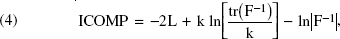
In light of such problems, researchers frequently use criteria such as Akaike's information criterion (AIC), Bayesian information criterion (BIC), consistent Akaike's information criterion (CAIC), and information complexity (ICOMP) to determine how many segments to retain and increase the number of segments until the criterion is minimized (Wedel and Kamakura 2000). The AIC, which is based on the use of generalized entropy as a goodness-of-fit measure, is calculated as

\begin{matrix} AIC = - 2 L + 2 k, \end{matrix}

(1)

where L is the value of the maximized log-likelihood function and k is the number of parameters required to estimate the model. The AIC is obtained by estimating twice the negentropy (the Kullback–Leibler information quantity, a measure of the distance between the fitted model and the true distribution), which is asymptotically equivalent to estimating minus twice the expected log-likelihood of the true distribution with parameters estimated by maximum likelihood (Bozdogan 1987). Akaike (1973) provides a derivation; see also Bozdogan (1987).

Various modifications of AIC have been proposed. Bozdogan (1981, 1992, 1994) argues that the marginal cost per parameter, the so-called magic number 2 in Equation 1, is not correct for finite mixture models. He conjectures that the likelihood ratio for comparing mixture model.¹ with K and k parameters is asymptotically distributed as a noncentral chi-square,

Bozdogan (1994) makes this conjecture in the context of mixtures of multivariate normal distributions and does not address whether it applies to mixtures of other distributions. He notes that proof of the conjecture in general is difficult within the context of the mixture model but that we can justify it on the basis of Feder's (1968) results and established asymptotic results in information theory.

- 2 \log λ \overset{a . d .}{\sim} χ_{v^{*}}^{'} (δ),

(2)

with noncentrality parameter δ and v^* = 2(K – k) degrees of freedom instead of the usual (K – k) degrees of freedom (as assumed in the derivation of AIC). If this is the case, we obtain 3 as the magic number in AIC in Equation 1 (for a proof, see Bozdogan 1994). We refer to this criterion as AIC3.

Another modification of AIC, the CAIC, makes AIC consistent without violating Akaike's principle of minimizing the Kullback-Leibler information quantity (Bozdogan 1987). By making the degrees of freedom of the likelihood ratio an increasing function of the sample size n (Kendall and Stuart 1967), such as v^* = (K – k) log n, instead of the usual (K – k) used in deriving AIC, we obtain

CAIC = - 2 L + k [(\log n) + 1] .

(3)

The CAIC therefore imposes a larger penalty per parameter than AIC, and the penalty grows with the sample size. (For a derivation of CAIC, see Bozdogan 1987, pp. 358–59.)

The key factor determining the relative quality of AIC, AIC3, and CAIC as segment retention criteria is the assumption made about the distribution of the likelihood ratio for finite mixtures. Because we cannot prove mathematically the exact form of the distribution, the simulation methods used in this study provide important insight on the matter.

As an alternative to AIC and CAIC, Bozdogan (1988a, 1990) developed a new entropic statistical complexity criterion called ICOMP. Although in the spirit of AIC, ICOMP removes any need to consider explicitly the parameter dimension of a model and adjusts automatically for the sample size. Rather than penalizing the log-likelihood for the number of parameters, ICOMP penalizes according to the interdependencies or correlations among the parameter estimates of the model. It is based on the properties of the estimated information matrix F, as follows:

\begin{matrix} \begin{matrix} \begin{matrix} ICOMP = - 2 L + k ln [\frac{tr (F^{- 1})}{k}] \end{matrix} - ln | F^{- 1} | \end{matrix} \end{matrix},

(4)

\begin{matrix} \hat{F} = - \frac{1}{n} \sum_{j = 1}^{n} [{\frac{\partial^{2} L (x_{j}, θ)}{\partial θ^{2}} |}_{θ = \hat{θ}}] \end{matrix},

(5)

and θ includes the segment-specific parameters and the parameters used to form the mixing weights (S – 1 parameters for an S-segment model). The first component of ICOMP measures the lack of fit of the model, and the second and third components measure the complexity of the estimated inverse-Fisher information matrix, which gives a scalar measure of the Cramer–Rao lower bound matrix of the model (Bozdogan 1992, 1994). In addition, ICOMP penalizes models that produce high variances in the parameter estimates through the second term and models in which the Hessian becomes nearly singular because of an increasing number of parameters through the third term (Wedel and Kamakura 2000).

The development of AIC, AIC3, CAIC, and ICOMP does not rely on a Bayesian approach. Schwarz (1978) develops a Bayes solution that consists of selecting the model that is a posteriori most probable. Known as BIC, the procedure differs from AIC only in that the dimension of the model is multiplied by log n rather than 2, which leads to lower dimensional models when there are eight or more observations. For large numbers of observations, the procedures differ markedly. Schwarz argues that under the assumptions set out in his analysis, AIC cannot be asymptotically optimal. The minimum description length criterion Rissanen (1987) developed using coding theory is identical in form to BIC.

No previous research has examined the performance of the log-likelihood value from the validation sample (LOGLV) as a segment retention criterion. The same logic that motivates an analyst to use a validation sample to indicate a model's suitability (e.g., the Bayesian cross-validated likelihood method by Rust and Schmittlein [1985]) also suggests that LOGLV could be used to determine the number of segments to retain in a finite mixture model. Indeed, AIC, BIC, CAIC, and ICOMP were first developed to select the proper subset of predictor variables to retain in regression models before they were used to select the number of components in a finite mixture model. Unlike the estimation sample log-likelihood, LOGLV may decrease when the number of segments increases, which may indicate misspecification. When consumers not used in the estimation process compose the validation sample, LOGLV is computed with the maximum likelihood estimates of parameters from the estimation sample, in exactly the same manner that the estimation sample log-likelihood is computed.² If the validation sample consists of additional purchases made by the same consumers used in model estimation, LOGLV may be calculated in a variety of ways. For example, consumers could be assigned to segments on the basis of the posterior probabilities using the estimation sample posterior probabilities, and each consumer's validation log-likelihood would be computed using the parameters from the segment with the highest posterior probability. Or an individual-level parameter vector could be computed as a convex combination of segment-level parameter estimates, for which the weights are posterior probabilities. Regardless of the exact form of LOGLV, the number of segments to retain in a finite mixture model is determined by increasing the number of segments until LOGLV is maximized.

Specifically, in this study we compute the likelihoods for each household–segment combination using the maximum likelihood estimates for each segment. We then create a weighted likelihood for each household using the estimated weights, take the logs, and sum across households.

We could also choose the number of segments on the basis of the separation between group centroids (Wedel and DeSarbo 1994). Celeux and Soromenho (1996) propose a normed entropy criterion (NEC) for the selection of the number of segments in finite mixture models, though it is unable to compare between S = 1 segments and S > 1 segments (except in certain circumstances). The NEC for some number of segments S is defined as

NEC (S) = \frac{E (S)}{L (S) - L (1)},

(6)

where L(S) and L(l) are the log-likelihoods for the S-segment and 1-segment solutions, and E(S) is the entropy for the S-segment model and indicates the separation between segments, defined as

\begin{matrix} \begin{matrix} E (S) = - \sum_{s = 1}^{S} \sum_{i = 1}^{n_{c}} π_{is} \ln π_{is} \end{matrix} \end{matrix},

(7)

where π_is is the posterior probability that consumer i belongs to segment s. The number of segments to retain in a finite mixture model is determined by increasing the number of segments until NEC is minimized.³

Another criterion unique to the segment retention problem is the minimum information ratio (MIR) proposed by Windham and Cutler (1992). Despite its initial appeal, proponents and others later reported substantial empirical drawbacks (for details, see Celeux and Soromenho 1996; Cutler and Windham 1994). Consequently, we do not consider MIR in our study.

There is no empirical evidence of whether these criteria perform satisfactorily in the context of finite mixture logit models applied to scanner panel data. Bozdogan (1988b) applies AIC to the task of selecting the proper order and subset of predictors in a loglinear model for a smoking risk data set but does not address the problem of segment retention. Given the widespread use of such criteria for segment retention in scanner data–based applications, the problem is important and in need of research.

Results of studies performed in contexts other than multinomial choice data vary widely, as we review subsequently, and thus are inconclusive. These studies consider a limited number of segment retention criteria and data characteristics (mostly multivariate normal data with no predictors). More important, because previous studies have appeared mostly in the statistics literature, there has been no investigation of factors of particular interest to marketing analysts using multinomial choice data, such as the number of choice alternatives, the number of choices per household, the error variance in the choice data, and the segment sizes.

The study by de Borrero (1993) examines the performance of selected fit criteria (AIC, CAIC, ICOMP, and MIR) for a univariate Poisson mixture model by varying the separation of the segments and the sample size. In that context, CAIC appears to be the best overall criterion. Rust and colleagues (1995) perform a simulation with regression models and find that BIC is the best overall model selection criterion in terms of selection accuracy, accuracy of posterior probabilities, and ease of use. However, their study was not conducted in the context of finite mixture models.

Bozdogan (1992, 1994) studies the problem of choosing the number of components in mixtures of multivariate normal distributions without predictor variables. The 1992 study compares AIC3, BIC, and ICOMP on two structures of simulated data. In both applications, all three criteria generally selected the same numbers of components, but in one application, none of the three selected the correct number of components. The 1994 study demonstrates the utility of ICOMP, AIC3, and CAIC in identifying the number of true segments using real medical data and two structures of simulated data.

Cutler and Windham (1994) study the performance of ten criteria in the context of mixtures of bivariate normal distributions with no predictors, varying the sample size (100, 200, 400), the number of components (2, 3, 4), the separation of components (0, 1, 2), and the specification of the covariance matrices (full, equal, and unequal, as is discussed in the next section). The performance of ICOMP is shown to be impressive, though they note that more research is needed on the criterion before generalizable conclusions can be drawn.

To summarize, the performance of segment retention criteria in the context of finite mixture logit models is unknown. In addition, no previous study has considered as many experimental factors of importance to marketing analysts with as many segment retention criteria. Our study manipulates seven experimental factors, whereas the largest previous study manipulates only four. Factors such as the number of choices per household, the number of choice alternatives, the error variance of the choices, and the minimum segment size are relevant in marketing settings but have not been considered in previous studies. Our study examines the performance of seven segment retention criteria, including two whose behaviors are largely untested and unknown. Given the gaps in the literature and the large variability in the findings of existing studies, there is no accepted solution to the segment retention problem. Answering the call of previous studies (e.g., DeSarbo et al. 1997), we examine the performance of segment retention criteria in an important analysis context in marketing.

Experimental Design

We test seven of the major segment retention criteria previously described (AIC, AIC3, BIC, CAIC, ICOMP, LOGLV, and NEC) in the context of multinomial choice data, described in detail subsequently.

We manipulate seven data characteristics. The factors and their levels, chosen from previous simulation studies by Vriens, Wedel, and Wilms (1996) and Andrews, Ainslie, and Currim (2002), are as follows:

Factor 1. The number of segments: 2 or 3;

Factor 2. The mean separation between segment coefficients: small (1.0), medium (1.5), or large (2.0).⁴

We first randomly generate the vector of parameters β₁ for Segment 1, as detailed subsequently. A vector of separations δ with mean 1.0, 1.5, or 2.0 (and standard deviations equal to 10% of the mean) is then randomly generated, as is a vector of signs S for δ. We do not want one segment to have all coefficients larger (or smaller) than another because this would indicate that one segment is more sensitive than another in every way. We then compute β₂ = β₁ + Sδ (element-by-element) and β₃ = β₁ – Sδ.

Factor 3. The number of households: 100 or 300;

Factor 4. The mean number of purchases per household: 5 or 10;

Factor 5. The number of choice alternatives: 3 or 6;

Factor 6. Error variance: standard (1.645) or high (50% higher than standard);

Factor 7. Minimum segment size: 5%–10%, 10%–20%, or 20%–30%.

The design is factorial, so with 3 replications (data sets) for each cell, we have a total of 3³2⁵ = 864 data sets. The number of replications (purchases) per individual in each data set is generated from a gamma distribution with a mean (and variance) of 5 or 10 (Factor 4).⁵ In addition, we generate purchases of 100 additional individuals not used in the estimation sample for the purposes of model validation (with the number of replications per individual again having a mean of 5 or 10).

The number of purchases per household in actual scanner panel data is often skewed in this manner, with some households having many purchases.

For each data set, we generate two binary variables (possibly but not necessarily representing promotional activities) and one variable with a standard normal distribution (possibly representing price) to represent the attributes consumers use to make choices. To improve generalizability, the parameter values are generated randomly for each segment and data set. Brand-specific constants (2 or 5 of them, depending on Factor 5) are generated uniformly to be in the range of −1 to 1 (they must be small enough that each brand has enough choices to allow accurate estimation of its constant). The coefficient for the normally distributed variable is generated in the range of −1 to −2.5. Coefficients for the two binary variables are between 1 and 2.5. These values are consistent with those observed in scanner panel applications. Consumers are assigned to segments on the basis of randomly determined segment sizes for each data set. The smallest segment will consist of 5%–10%, 10%–20%, or 20%–30% of the sample, depending on the level of Factor 7. Given a consumer's segment assignment, we use segment-specific parameters to compute deterministic utilities, to which double exponential errors (with variances determined by Factor 6) are added. The consumer is assumed to choose the brand with the highest logit choice probability.

Expected Results

The most comprehensive simulation study to date (Cutler and Windham 1994) suggests that the type of model affects the performance of segment retention criteria. That study examined three mixtures of bivariate normal distributions: (1) the full model, in which the true covariance matrices and segment sizes were generated randomly; (2) the unequal model, in which the true covariance matrices were set to identity matrices, but the segment sizes were generated randomly; and (3) the equal model, in which the true covariance matrices were set to identity matrices and the segments sizes were set to 1/k, where k is the number of segments. The AIC showed a consistent tendency to overfit across experimental conditions with the full model but not with the equal and unequal models. The AIC3 tended to underfit with the full model but performed well with the equal and unequal models. The BIC almost never overfitted the number of segments but had alarmingly high rates of underfitting with the full model. Although the CAIC was not tested, it would have underfitted the number of segments as least as badly as BIC because it has a larger penalty per parameter. The ICOMP criterion did not have a systematic tendency to underfit or overfit, in that it underfit the full model but overfit the equal model somewhat more than the other criteria.

Of the three mixture models Cutler and Windham (1994) test, our multinomial logit model most closely resembles the unequal model because (1) the parameter vectors for each segment must be estimated, (2) covariances are not applicable in multinomial logit choice models and therefore do not require estimation, and (3) the segment sizes must be estimated. If this is the case, on the basis of Cutler and Wind-ham's results, we expect ICOMP to have the highest success rates in general, with AIC, AIC3, BIC, and CAIC (in that order) resulting in more severe underfitting compared with ICOMP. On the basis of these results, we do not expect any of the criteria to have a tendency to overfit. There is no basis for speculating about the relative performance of LOGLV and NEC, though given that NEC cannot be calculated for one-segment models, there is an increased chance that it will overfit the number of segments (or at least a decreased chance that it will underfit).

In general, we expect the segment retention criteria to underfit more when the number of true segments is three rather than two, the separation between segments is smaller, the number of households is smaller, the number of choices per household is smaller, the number of choice alternatives is larger, the error variance is larger, and the minimum segment size is smaller. Bozdogan (1992) and Cutler and Windham (1994) both find that criteria tend to underfit more when the true number of segments is larger. Cutler and Windham find more underfitting with three segments than with two. They also provide support for the assertion that segments that are closer together are more difficult to detect. With smaller sample sizes, additional segments capture fewer households, and consequently the incremental contribution to the likelihood is smaller, making justification of additional segments more difficult. Bozdogan (1987) argues that as the number of observations becomes large, the probability of underfitting a model will diminish, especially for consistent criteria (BIC and CAIC). More parameters are required when there are more choice alternatives, which should lead to increased underfitting. Larger error variance, in our experience, makes the identification of segments more difficult, which results in a tendency to underfit. Finally, smaller segments should be more difficult to detect than larger segments, which leads to increased underfitting.

Summary of Results

We measure the performance of the various segment retention criteria by their success rates, or the percentages of data sets in which the criteria identify the true number of segments. Given two criteria with similar success rates, we then prefer underfitting to overfitting. Our research for this study shows that overfitting produces larger parameter bias at the individual level than underfitting does. Although we might not expect a priori that overfitting would produce larger parameter bias than underfitting, the explanation seems to be that overfitting sometimes produces very small segments with large or unstable parameter values, which can result in severe bias. Cutler and Windham (1994, p. 154) also prefer underfitting to overfitting, especially for small sample sizes and components that are not well separated.

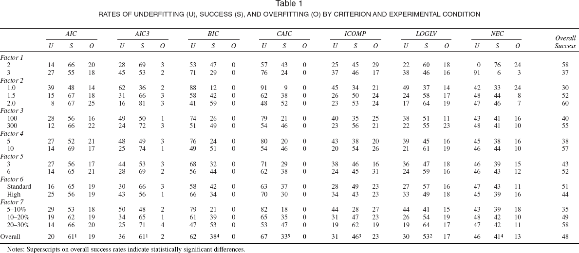
Tables 1 and 2 present the results of the simulation experiment. Table 1 shows the success rates (S) of each criterion by experimental condition, along with the rates of underfitting (U) and overfitting (O). For example, AIC correctly identified the number of segments in 66% of data sets with two components (Factor 1), underfitted the number of components in 14% of these data sets, and overfitted the number of components in 20% of these data sets. At the bottom of Table 1, we use z-tests to test for statistically significant differences among the overall success rates of the criteria, based on the least significant difference rule. For example, AIC and AIC3 have the best overall success rates, followed by LOGLV, ICOMP, BIC and NEC, and CAIC. In Table 2, we meta-analyze the results by fitting logit models to the success data from Table 2 (where 1 = success); the predictors are dummy variables that represent the simulation design factors. For example, because F1 = 1 when the number of segments is two, AIC has a significantly higher success rate when there are two segments (66%, Table 1) than when there are three segments (55%). Separate logit models are fit to the data for each criterion, which is conceptually equivalent to fitting a common model to all data and including criteria by factor interactions, as other recent studies have done (Andrews, Ainslie, and Currim 2002; Andrews, Ansari, and Currim 2002; Vriens, Wedel, and Wilms 1996).

Surprisingly, AIC3 has the best overall performance in the simulation. Although AIC has an equally good success rate (61%, Table 1), AIC3 has low rates of overfitting (2%), and the rate of overfitting is much higher for AIC (19%). As we mentioned previously, we prefer to avoid criteria that overfit the true number of segments because parameter bias is much more likely with overfitted models. The AIC3 typically has success rates at or near the best in all experimental conditions, though AIC has higher success rates for some experimental conditions (at the expense of significant overfitting).

The LOGLV criterion has the second best success rate, though overfitting is higher than we prefer (17%). The ICOMP criterion has lower success rates than AIC3, AIC, and LOGLV, which is not consistent with the performance of the criterion in the context of mixtures of bivariate normal distributions (Cutler and Windham 1994). We discuss this finding in the next section.

The BIC is better than only CAIC for the multinomial data. As expected, BIC underfits significantly (62%) but never overfits. The CAIC underfits even more severely (67%) and is the least effective criterion overall.

The logit meta-analysis (Table 2) confirms that, as expected, the criteria generally have significantly higher success rates when there are two segments rather than three, there is larger separation between segments, sample sizes are larger, there are more choices per household, error variance is smaller, and the segments are larger. There was one unexpected finding: Success rates are generally higher when there are six choice alternatives rather than three. We expected more underfitting when there were six alternatives, but the opposite is true. Perhaps this is because the fit of the model is better when there are three alternatives rather than six (the consumer has fewer choice options, which makes prediction easier), which leaves less opportunity for improvement in fit by increasing the number of segments. Overall, the logit results are remarkably consistent with our expectations.

To investigate how well the simulation results generalize to data sets with more latent segments, we generated 100 additional data sets with six true segments instead of two or three.⁶ The success rates were as follows: AIC 52%, AIC3 59%, BIC 54%, CAIC 53%, ICOMP 44%, LOGLV 54%, and NEC 2%. The rates of underfitting were as follows: AIC 17%, AIC3 22%, BIC 36%, CAIC 38%, ICOMP 28%, LOGLV 16%, and NEC 98%. Thus, even with six segments, AIC3 still appears to be a good segment retention criterion. With an average of 4000 purchases per data set, however, there is less variation among the success rates of the segment retention criteria (with the exception of NEC). The consistent criteria (BIC and CAIC), in particular, perform better than would be expected from the larger simulation study.

The mean separation between segments was 2.0 (level three of Factor 2) because it may be unrealistic to recover six segments that are close together. The sample size was set at 400 because it is not realistic to attempt to identify six segments with 100 (or maybe even 300) households. Likewise, the mean number of purchases per household was set at 10 (level two of Factor 4) by the same reasoning. We assumed six alternatives (level two of Factor 5), standard error variance (level one of Factor 6), and a minimum segment size of 10%.

Table 1

Rates of Underfitting (U), Success (S), and Overfitting (O) by Criterion and Experimental Condition

	AIC			AIC3			BIC			CAIC			ICOMP			LOGLV			NEC			Overall Success
	U	S	O	U	S	O	U	S	O	U	S	O	U	S	O	U	S	O	U	S	O	Overall Success
Factor 1
2	14	66	20	28	69	3	53	47	0	57	43	0	25	45	29	22	60	18	0	76	24	58
3	27	55	18	45	53	2	71	29	0	76	24	0	37	46	17	38	46	16	91	6	3	37
Factor 2
1.0	39	48	14	62	36	2	88	12	0	91	9	0	45	34	21	49	37	14	42	33	24	30
1.5	15	67	18	31	66	3	58	42	0	62	38	0	26	50	24	24	58	17	48	44	8	52
2.0	8	67	25	16	81	3	41	59	0	48	52	0	23	53	24	17	64	19	47	46	7	60
Factor 3
100	28	56	16	49	50	1	74	26	0	79	21	0	40	35	25	38	51	11	43	41	16	40
300	12	66	22	24	72	3	51	49	0	54	46	0	23	56	21	22	55	23	48	41	10	55
Factor 4
5	27	52	21	48	49	3	76	24	0	80	20	0	43	38	20	39	45	16	45	38	16	38
10	14	69	17	25	74	1	49	51	0	54	46	0	20	54	26	21	61	19	46	44	10	57
Factor 5
3	27	56	17	44	53	3	68	32	0	71	29	0	38	46	16	36	47	18	46	39	15	43
6	14	65	21	28	69	2	56	44	0	62	38	0	24	45	31	24	59	16	46	43	12	52
Factor 6
Standard	16	65	19	30	66	3	58	42	0	63	37	0	28	49	23	27	57	16	47	43	11	51
High	25	56	19	43	56	1	66	34	0	70	30	0	34	43	23	33	49	18	45	39	16	44
Factor 7
5–10%	29	53	18	50	48	2	79	21	0	82	18	0	44	28	27	44	41	15	43	39	18	35
10–20%	19	62	19	34	65	1	61	39	0	65	35	0	31	47	23	26	54	19	48	42	10	49
20–30%	14	66	20	25	71	4	47	53	0	53	47	0	19	62	19	19	64	17	47	42	11	58
Overall	20	611	19	36	611	2	62	384	0	67	335	0	31	463	23	30	532	17	46	414	13	48

Notes: Superscripts on overall success rates indicate statistically significant differences.

Table 2

Meta-Analysis Of Results: Logit Results by Criterion and Experimental Condition

	AIC		AIC3		BIC		CAIC		ICOMP		LOGLV		NEC
Factor	B	Significance	B	Significance	B	Significance	B	Significance	B	Significance	B	Significance	B	Significance
F1	.513	.001	1.103	.000	1.426	.000	1.594	.000	–.057	.706	.631	.000	4.061	.000
F2		.000		.000		.000		.000		.000		.000		.000
F2(1)	–.872	.000	–2.879	.000	–3.728	.000	–3.718	.000	–.932	.000	–1.247	.000	–1.065	.000
F2(2)	–.017	.926	–1.074	.000	–1.169	.000	–.980	.000	–.149	.413	–.262	.148	–.191	.449
F3	–.470	.002	–1.530	.000	–1.811	.000	–2.031	.000	–.986	.000	–.220	.139	–.080	.689
F4	–.831	.000	–1.708	.000	–2.115	.000	–2.136	.000	–.773	.000	–.716	.000	–.443	.029
F5	–.448	.003	–1.134	.000	–.954	.000	–.790	.000	.057	.706	–.610	.000	–.322	.110
F6	.383	.010	.725	.000	.657	.001	.633	.002	.306	.043	.351	.018	.322	.110
F7		.003		.000		.000		.000		.000		.000		.445
F7(1)	–.604	.001	–1.558	.000	–2.545	.000	–2.470	.000	–1.600	.000	–1.039	.000	–.270	.272
F7(2)	–.220	.233	–.430	.057	–1.034	.000	–.962	.000	–.720	.000	–.445	.015	.000	1.000
Constant	1.480	.000	3.996	.000	3.217	.000	2.667	.000	1.646	.000	1.416	.000	–2.073	.000
–2LOGL	1052		761		663		632		1025		1052		648
%Correct	68.5		79.4		81.8		82.6		68.8		67.4		85.2

Factor 1: Number of components: 2 (1 for F1) or 3 (0 for F1).

Factor 2: Mean separation between component coefficients: 1.0 (1 for F2(1)), 1.5 (1 for F2(2)), or 2.0 (0).

Factor 3: Sample size: 100 (1 for F3) or 300 (0 for F3).

Factor 4: Number of choices per household: mean of 5 (1 for F4) or 10 (0 for F4).

Factor 5: Number of choice alternatives: 3 (1 for F5) or 6 (0 for F5).

Factor 6: Error variance: standard (1 for F6) or high (0 for F6).

Factor 7: Minimum segment size: 5%–10% (1 for F7(1)), 10%–20% (1 for F7(2)), or 20%-30% (0).

Notes: Dependent variable is 0–1 indicator of success in identifying the correct number of segments, with success = 1.

Conclusion

Despite the emergence of Bayesian error components models and other random coefficient procedures in recent years, applications of finite mixture models still accumulate (Wedel and Kamakura 2000) and should continue to do so given new evidence of their effectiveness (Andrews, Ansari, and Currim 2002). As the range of application of finite mixture models continues to extend to the domains of cluster analysis (McLachlan and Basford 1988; Wedel and Kamakura 2000), multidimensional scaling (Andrews and Manrai 1999; Chintagunta 1994; Wedel and DeSarbo 1996), and conjoint analysis (Andrews and Manrai 1999; DeSarbo et al. 1992; Fader and Hardie 1996; Kamakura, Wedel, and Agrawal 1994), the models will likely become more important to applied and theoretical research in marketing.

This study shows that AIC with a per parameter penalty factor of three rather than the traditional value of two is the best segment retention criterion to use with a large variety of data configurations. Because AIC3 differs from AIC and CAIC only in the assumption made about the distribution of the likelihood ratio in finite mixtures (in which parameters are often on the boundaries of parameter spaces), we conclude that the actual distribution of the likelihood ratio is better approximated as a noncentral chi-square with 2(K – k) degrees of freedom. Currently, AIC3 is rarely, if ever, applied in the marketing literature. With very large sample sizes, the consistent criteria (BIC and CAIC) also perform well, as suggested by Bozdogan (1987).

Because the results of this study conducted in the context of multinomial choice data are not completely consistent with results of prior studies conducted with mixtures of other distributions, it may be that no one segment retention criterion is best for all types of mixtures in all situations. Perhaps it is not realistic to assume that there is one best criterion to use for all scenarios; even different specifications of a bivariate normal mixture produced varying results in Cutler and Windham's (1994) study. We are currently running simulations with mixtures of other types of distributions to test the generality of the findings on AIC3. Also, because no criterion has been perfectly capable of identifying the correct number of segments, additional research should continue to search for better criteria for segment retention. For analysts, another potentially important factor that was not studied directly in these simulations was distributional misspecification, that is, when the distribution of the data does not match that of the model. A manager, in contrast, must consider the costs and benefits (in dollars and cents) of under- or overestimating the true number of segments. By beginning to address the last major statistical deficiency with finite mixture models, the segment retention problem, researchers can significantly increase the utility of logit models for managers who make segmentation, new product development, and marketing-mix decisions.

References

Abramson

Charles

, Andrews

Rick L.

, Currim

Imran S.

, and Jones

Morgan

(2000), “Parameter Bias from Unobserved Effects in the Multinomial Logit Model of Consumer Choice,” Journal of Marketing Research, 37(November), 410–26.

Abramson

Charles

, Buchmueller

Thomas

, and Currim

Imran S.

(1998), “Models of Health Plan Choice,” European Journal of Operational Research, 111(December), 228–47.

Aitkin

, Anderson

, and Hinde

(1981), “Statistical Modeling of Data on Teaching Styles,” Journal of Royal Statistical Society, A144, 419–61.

Akaike

Hirotugu

(1973), “Information Theory and an Extension of the Maximum Likelihood Principle,” in Second International Symposium on Information Theory, Petrov

B.N.

, and Csaki

B.F.

, eds. Budapest: Academiai Kiado, 267–81.

Andrews

Rick L.

, Ainslie

Andrew

, and Currim

Imran S.

(2002), “An Empirical Comparison of Logit Choice Models with Discrete Versus Continuous Representations of Heterogeneity,” Journal of Marketing Research, 39(November), 479–87.

Andrews

Rick L.

, Ansari

Asim

, and Currim

Imran S.

(2002), “Hierarchical Bayes Versus Finite Mixture Conjoint Analysis Models: A Comparison of Fit, Prediction, and Partworth Recovery,” Journal of Marketing Research, 39(February), 87–98.

Andrews

Rick L.

, and Currim

Imran S.

(2002), “Identifying Segments with Identical Choice Behaviors Across Product Categories: An Inter-category Logit Mixture Model,” International Journal of Research in Marketing, 19(March), 65–79.

Andrews

Rick L.

, and Manrai

Ajay K.

(1999), “MDS Maps for Product Attributes and Market Response: An Application to Scanner Panel Data,” Marketing Science, 18(4), 584–604.

Bozdogan

Hamparsum

(1981), “Multi-Sample Cluster Analysis and Approaches to Validity Studies in Clustering Individuals,” doctoral thesis, Department of Mathematics, University of Illinois at Chicago.

10.

Bozdogan

Hamparsum

(1987), “Model Selection and Akaike's Information Criterion (AIC): The General Theory and Its Analytical Extensions,” Psychometrika, 52(3), 345–70.

11.

Bozdogan

Hamparsum

(1988a), “ICOMP: A New Model Selection Criterion,” in Classification and Related Methods of Data Analysis, Hans

H. Bock

, ed. Amsterdam: North-Holland, 599–608.

12.

Bozdogan

Hamparsum

(1988b), “Selecting Loglinear Models and Subset Selection of Variables in Multiway Contingency Tables Using Akaike's Information Criterion (AIC),” in Classification and Related Methods of Data Analysis, Hans

H. Bock

, ed. Amsterdam: North-Holland, 609–16.

13.

Bozdogan

Hamparsum

(1990), “On the Information-Based Measure of Covariance Complexity and its Application to the Evaluation of Multivariate Linear Models,” Communications in Statistics, Theory, and Methods, 19(1), 221–78.

14.

Bozdogan

Hamparsum

(1992), “Choosing the Number of Component Clusters in the Mixture-Model Using a New Informational Complexity Criterion of the Inverse-Fisher Information Matrix,” in Information and Classification: Concepts, Methods and Applications, Opitz

, Lausen

, and Klar

, eds. New York: Springer-Verlag, 40–54.

15.

Bozdogan

Hamparsum

(1994), “Mixture-Model Cluster Analysis using Model Selection Criteria and a New Informational Measure of Complexity,” in Proceedings of the First US/Japan Conference on the Frontiers of Statistical Modeling: An Informational Approach, Vol. 2, Bozdogan

, ed. Boston: Kluwer Academic Publishers, 69–113.

16.

Celeux

Gilles

, and Soromenho

Gilda

(1996), “An Entropy Criterion for Assessing the Number of Clusters in a Mixture Model,” Journal of Classification, 13(2), 195–212.

17.

Chintagunta

Pradeep K.

(1994), “Heterogeneous Logit Model Implications for Brand Positioning,” Journal of Marketing Research, 31(May), 304–11.

18.

Chintagunta

Pradeep K.

, Jain

Dipak C.

, and Vilcassim

Naufel J.

(1991), “Investigating Heterogeneity in Brand Preferences in Logit Models for Panel Data,” Journal of Marketing Research, 28(November), 417–528.

19.

Cutler

, and Windham

M.P.

(1994), “Information-Based Validity Functionals for Mixture Analysis,” in Proceedings of the First US/Japan Conference on the Frontiers of Statistical Modeling: An Informational Approach, Vol. 2, Bozdogan

, ed. Boston: Kluwer Academic Publishers, 149–70.

20.

de Borrero

Melinda Smith

(1993), “Determining the Number of Mixture Components and a Poisson-Multinomial Logit Mixture Model Application in Marketing Research,” doctoral dissertation, Department of Marketing, University of South Carolina.

21.

DeSarbo

Wayne S.

, Ansari

Asim

, Chintagunta

Pradeep

, Himmelberg

Charles

, Jedidi

Kamel

, Johnson

Richard

, Kamakura

Wagner

, Lenk

Peter

, Srinivasan

Kannan

, and Wedel

Michel

(1997), “Representing Heterogeneity in Consumer Response Models,” Marketing Letters, 8(3), 335–48.

22.

DeSarbo

Wayne S.

, Wedel

Michel

, Vriens

Marco

, and Ramaswamy

Venkatram

(1992), “Latent Class Metric Conjoint Analysis,” Marketing Letters, 3(3), 273–88.

23.

Dillon

William R.

, Böckenholt

Ulf

, de Borrero

Melinda Smith

, Bozdogan

Ham

, DeSarbo

Wayne

, Gupta

Sunil

, Kamakura

Wagner

, Kumar

Ajith

, Ramaswamy

Venkatram

, and Zenor

Michael

(1994), “Issues in the Estimation and Application of Latent Structure Models of Choice,” Marketing Letters, 5(4), 323–34.

24.

Dillon

William R.

, and Kumar

Ajith

(1994), “Latent Structure and Other Mixture Models in Marketing: An Integrative Survey and Overview,” in Advanced Methods of Marketing Research, Richard

P. Bagozzi

, ed. Malden, MA: Blackwell Publishers, Ltd., 295–351.

25.

Fader

Peter S.

, and Hardie

Bruce G.S.

(1996), “Modeling Consumer Choice Among SKUs,” Journal of Marketing Research, 33(November), 442–52.

26.

Feder

P.I.

(1968), “On the Distribution of the Log Likelihood Ratio Test Statistic When the True Parameter Is ‘Near’ the Boundaries of the Hypothesis Regions,” Annals of Mathematical Statistics, 39, 2044–55.

27.

Gupta

Sachin

, and Chintagunta

Pradeep K.

(1994), “On Using Demographic Variables to Determine Segment Membership in Logit Mixture Models,” Journal of Marketing Research, 31(February), 128–36.

28.

Hope

A.C.A.

(1968), “A Simplified Monte Carlo Significance Test Procedure,” Journal of the Royal Statistical Society, Series B (30), 582–98.

29.

Jain

Dipak C.

, Vilcassim

Naufel J.

, and Chintagunta

Pradeep K.

(1994), “A Random-Coefficients Logit Brand-Choice Model Applied to Panel Data,” Journal of Business & Economic Statistics, 12(July), 317–28.

30.

Kamakura

Wagner A.

, Kim

Byung-Do

, and Lee

Jonathan

(1996), “Modeling Preference and Structural Heterogeneity in Consumer Choice,” Marketing Science, 15(2), 152–72.

31.

Kamakura

Wagner A.

, and Russell

Gary J.

(1989), “A Probabilistic Choice Model for Market Segmentation and Elasticity Structure,” Journal of Marketing Research, 26(November), 379–90.

32.

Kamakura

Wagner A.

, and Russell

Gary J.

(1993), “Measuring Brand Value with Scanner Data,” International Journal of Research in Marketing, 10(1), 9–22.

33.

Kamakura

Wagner A.

, Wedel

Michel

, and Agrawal

Jagadish

(1994), “Concomitant Variable Latent Class Models for Conjoint Analysis,” International Journal of Research in Marketing, 11(5), 451–64.

34.

Kendall

M.G.

, and Stuart

M.A.

(1967), The Advanced Theory of Statistics, Vol. 2, 2d ed. New York: Hafner Publishing.

35.

McLachlan

Geoffrey J.

(1987), “On Bootstrapping the Likelihood Ratio Test Statistic for the Number of Components in a Normal Mixture,” The Journal of the Royal Statistical Society, C36(3), 318–24.

36.

McLachlan

Geoffrey J.

, and Basford

Kaye E.

(1988), Mixture Models: Inference and Applications to Clustering. New York: Marcel Dekker, Inc.

37.

Rissanen

(1987), “Stochastic Complexity,” Journal of the Royal Statistical Society, Series B, 49(3), 223–39.

38.

Roy

Rishin

, Chintagunta

Pradeep K.

, and Haldar

Sudeep

(1996), “A Framework for Investigating Habits, ‘The Hand of the Past,’ and Heterogeneity in Dynamic Brand Choice,” Marketing Science, 15(3), 280–99.

39.

Rust

Roland T.

, and Schmittlein

David C.

(1985), “A Bayesian Cross-Validated Likelihood Method for Comparing Alternative Specifications of Quantitative Models,” Marketing Science, 4(1), 20–40.

40.

Rust

Roland T.

, Simester

Duncan

, Brodie

Roderick J.

, and Nilikant

(1995), “Model Selection Criteria: An Investigation of Relative Accuracy, Posterior Probabilities, and Combinations of Criteria,” Management Science, 41(February), 322–33.

41.

Schwarz

Gideon

(1978), “Estimating the Dimension of a Model,” The Annals of Statistics, 6(2), 461–64.

42.

Vriens

Marco

, Wedel

Michel

, and Wilms

Tom

(1996), “Metric Conjoint Segmentation Methods: A Monte Carlo Comparison,” Journal of Marketing Research, 33(February), 73–85.

43.

Wedel

Michel

, and DeSarbo

Wayne S.

(1994), “A Review of Recent Developments in Latent Class Regression Models,” in Advanced Methods of Marketing Research, Richard

P. Bagozzi

, ed. Malden, MA: Blackwell Publishers, Ltd., 352–88.

44.

Wedel

Michel

, and DeSarbo

Wayne S.

(1996), “An Exponential-Family Multidimensional Scaling Mixture Methodology,” Journal of Business & Economic Statistics, 14(October), 447–59.

45.

Wedel

Michel

, and Kamakura

Wagner A.

(2000), Market Segmentation: Conceptual and Methodological Foundations, 2d ed. Boston: Kluwer Academic Publishers.

46.

Windham

M.P.

, and Cutler

(1992), “Information Ratios for Validating Mixture Analyses,” Journal of the American Statistical Association, 87(420), 1188–92.