Modeling Preferences for Common Attributes in Multicategory Brand Choice

Abstract

The authors propose a multicategory brand choice model based on the conceptualization that the intrinsic utility for a brand is a function of underlying attributes, some of which are common across categories. The premise is that household preferences for attributes that are common across categories are likely to be correlated. The model that the authors develop projects the unobserved preferences for attributes to a lower dimensional space of unobserved factors. The factors are interpretable as household “traits” that transcend categories, and they can be used to predict preferences for attributes in new categories. The authors apply the proposed model to household panel data for three closely related snack categories and for two less-related food categories. The authors find strong correlations in preferences for product attributes such as brand names and low fat or fat free. This study demonstrates that these high correlations in product attribute preferences across categories are useful in targeting activities in existing and new categories.

A vast literature in marketing describes brand choice behavior within individual product categories. A consistent empirical finding across multiple studies is that consumer heterogeneity in brand preferences and responsiveness to marketing-mix variables explains a substantial part of the variation in brand choices of households. In other words, consumers are very different from one another within each category. An important question that has intrigued marketing researchers is whether a household exhibits similarities in its choice behavior across seemingly disparate categories. In other words, are consumers' buying behaviors and sensitivities to marketing-mix variables determined primarily by household-specific factors or by category-specific characteristics? Although this question has long been of interest (see, e.g., Blattberg, Peacock, and Sen 1976), appropriate methodologies to address the issue have only recently been developed (Ainslie and Rossi 1998; hereinafter AR). Using data from five product categories, AR find substantial correlations in price, display, and feature sensitivity of households. Similarly, Erdem (1998) and Erdem and Winer (1999) find that consumers' preferences for a brand name are correlated across categories. Such findings have sparked interest in the development of multicategory choice models—that is, models in which consumers' preferences for brands and their responsiveness to marketing activities in each category have a joint distribution that allows correlation across categories.

The problem of finding and explaining generalities in consumers' buying propensities across product categories is of intrinsic academic interest. For example, the discovery of empirical patterns can trigger the development of new theories of consumer behavior and has important implications for marketing practice. The processing of consumer packaged goods is a highly concentrated business, with only a few companies accounting for a large share of the overall global market (Rogers 2001). Each of the major manufacturers, such as Procter & Gamble, Unilever, General Mills, and Kraft, owns brands in a vast number of product categories. The downstream customers of these manufacturers are large supermarket chains, which are multicategory firms as well. For these firms, developing an understanding of consumers' preferences or traits that transcends product categories can be a source of strategic advantage. Potential application areas include umbrella branding and advertising (Erdem 1998; Erdem and Sun 2002), brand equity and its extendability (Park and Srinivasan 1994), cross-category promotions (Chintagunta and Haldar 1998), new product targeting (the current article), and so forth.

In this article, we focus on the use of observed household purchase data to analyze preferences in multiple categories. In packaged goods markets, the availability of good household panel data from marketing research providers, such as ACNielsen and Information Resources Inc., or from retailers' frequent-shopper programs has facilitated such an endeavor. However, the analysis of consumers' choices in disparate product categories poses difficult modeling challenges. A fundamental issue that must be addressed is how to correlate consumers' preferences for products that fall in different product categories and are therefore like apples and oranges. Note that the set of marketing-mix variables is typically the same across supermarket categories (i.e., in-store prices, feature advertising, and in-store displays). Therefore, similarities in a consumer's choice behavior across seemingly different categories arise in part because of common marketing-mix variables. It is not surprising that the majority of prior research on cross-category comparisons has focused on investigating commonalities in marketing-mix sensitivities (Ainslie and Rossi 1998; Bell, Chiang, and Padmanabhan 1999; Deepak, Ansari, and Gupta 2002; Iyengar, Ansari, and Gupta 2003; Kim Srinivasan, and Wilcox 1999).¹

Note that Van Heerde, Gupta, and Wittink (2003) provide a different substantive interpretation of Bell, Chiang, and Padmanabhan's (1999) results in terms of the decomposition of the sales effects of promotional activities.

We conceptualize product alternatives in individual product categories as bundles of attributes, some of which are common across categories. (In the context of modeling brand choice in individual categories, Fader and Hardie [1996] propose the idea of viewing stockkeeping unit [SKU] alternatives as attribute bundles.) For example, within any typical packaged goods category, brand name and pack size are common attributes to all product alternatives, with each alternative characterized by its “level” of each attribute. Specific subgroups of categories may share many other attributes. For example, an attribute shared by products in packaged foods categories, such as sliced cheese, mayonnaise, ice cream, and milk, is the fat content. Another attribute that characterizes products in multiple food categories is “organic” or “natural.” A consumer's preference for a product in a category can then be viewed as a function of preferences for the attribute levels of the product and the consumer's sensitivity to the values of the marketing-mix variables. An advantage of using the attribute structure in our multicategory setting is that similarities in a consumer's choice behavior across seemingly different categories could arise not only as a result of marketing-mix variables but also as a result of a consumer's preferences for attributes that are common across categories. For example, a consumer who prefers to eat healthy food is likely to exhibit a preference for “better-for-you” products, which include fat-free, low-fat, or light products in multiple food categories. Similarly, “low-carb” consumers or “green” consumers may exhibit similarities in their brand choices across categories, driven by their desire for low-carbohydrate or environmentally friendly products.

We propose a multicategory brand choice model that captures this conceptualization of attribute-based preferences. A consumer's intrinsic utility for a product is a function of the utilities of the underlying attributes of the product and the consumer's sensitivity to marketing-mix variables. Heterogeneity across households is captured by allowing the full vector of parameters to be a function of observed household characteristics and unobserved components. Our main focus is on the estimation of the joint distribution of preferences for attributes and the estimation of the degree of correlation in preferences for these attributes across product categories. The major problem in the estimation of multicategory brand choice models is how to model the joint distribution of preferences in a way that is parsimonious yet not too restrictive. Our approach is to impose a factor structure on the covariance matrix of the parameters, which enables household-level preferences to be modeled as a function of observable household characteristics and a small number of unobservable household-specific “factors.” Together, these observed and unobserved household-specific components capture the dependence both within and across product categories.

The proposed approach has several advantages over existing models that try to understand cross-category purchase behavior. For example, a common approach used in the literature involves estimating separate brand choice models for each category and computing correlations in parameter estimates across categories ex post (e.g., Kim, Srinivasan, and Wilcox 1999). However, as AR (1998) point out, this approach is not efficient, and it underestimates the true cross-category correlations. Instead, AR propose a variance component approach to model multicategory brand choices. Our model is a generalization of AR's model in several ways:

•

AR restrict cross-category correlations in the preference vector to the marketing-mix variables, whereas we allow for correlations in the full vector of product preferences. This relaxation yields greater insights into the drivers of cross-category similarities in choice behavior and, as we show in the section “Cross-Category Targeting Applications,” is also useful for many marketing applications.

•

We allow the covariance matrix between attribute preferences to vary across different pairs of categories. That is, if there are, for example, three categories, we allow the covariance matrix between preferences for attributes in Categories 1 and 2 to be different from the covariance matrix between preferences in Categories 1 and 3. For example, although a household may prefer fat-free products in several food categories, in certain food categories, it may prefer “regular” products because children are the primary consumers of these products in the household. Similarly, Dhar and Simonson (1999) note that consumption of an attribute in one category may be “balanced” by the consumption of that attribute in other categories within consumption episodes, and to the extent consumers can anticipate this, it may affect their brand choices when shopping. We accomplish this by giving the unobservable part of preferences a factor structure with loading matrices that vary across categories.

•

By relying on a variance component approach, AR are restricted to modeling cross-category correlations for attribute vectors with the same dimensionality in each category. Because they are interested only in cross-category correlations in marketing-mix variables (which are usually the same across categories), this does not create a problem. However, we wish to model cross-category correlations between attribute vectors whose dimensionality potentially varies across categories. Our approach, which is based on factors and loading matrices, easily allows for this.

•

AR's variance component approach constrains the correlations in preferences to be positive, whereas our approach does not impose such restrictions.

•

AR model the vector of marketing-mix responsiveness parameters as a function of observable demographic characteristics whose effects are assumed (for parsimony) to be category invariant, whereas we allow the demographic effects to vary across categories.

Our proposed model allows household-level preferences to be a function of observable household characteristics and a small number of unobservable household-specific factors. Although our approach does not require the factors to be interpreted—they can be considered simply a tool to model dependence—it is potentially relevant from a marketing perspective to label the factors. The factors can be interpreted as category-stable preferences, which we term “consumer traits.” Similar to classical factor analysis, a small set of labeled factors facilitates communication and discussion of model results among users.

The factors play another important role. It is well known that demographic variables are poor predictors of preferences that are estimated on scanner panel data (see, e.g., Gupta and Chintagunta 1994; Rossi, McCulloch, and Allenby 1996). Consistent with this literature, we find that demographic variables explain relatively little of the overall variation in preferences in our data. In contrast, we find that the factors explain most of the variation in preferences for many of the included attributes. The problem is that the factors are not directly observable. However, if purchase history data are available for a substantial fraction of consumers in the target segment, such as through frequent-shopper cards, it would be possible to use our factor model to infer household-specific factor estimates. Furthermore, if these factors are important in the description of covariation in preferences for attributes across product categories (our results show that this is indeed the case), it would be possible to use these estimates to predict household demand in new product categories. Thus, from a managerial perspective, our model is well suited for firms that want to gain greater advantage from the information contained in frequent-shopper databases that track purchase histories for all their customers.

We present two applications of our model: The first is to household purchase data for a set of three closely related snack food categories (potato chips, tortilla chips, and pretzels) that are purchased for similar consumption needs. Moreover, there are many common attributes across the three categories. In these categories, we find significant correlations in preferences for product attributes such as brand names, pack sizes, and no salt, as well as price sensitivities. Second, to explore the robustness of the multicategory model, we apply it to two food categories (sliced cheese and mayonnaise) that are purchased for unrelated consumption needs and have fewer common attributes. In this application, we also find significant correlations in preferences for attributes such as fat free and private label, as well as marketing-mix sensitivities. These high correlations in product attribute preferences across categories create the opportunity for important cross-category targeting applications. For example, consider a retailer that introduces a new private label brand in a category. Although the retailer may not have any information on potential targets in this category, it can use information on households in other categories in which the retailer already sells the private label to infer potential targets for its brand in the new category. Similarly, households that prefer the diet or low-fat attribute in, for example, cheese and mayonnaise categories could be potential targets for entirely new product categories, such as Lean Cuisine-type frozen dinners or low-fat frozen pizzas. We illustrate these potential benefits in the section “Cross-Category Targeting Applications.”

We organize the rest of the article as follows: We begin by describing our modeling approach, and we outline the main aspects of the estimation procedure. Then, we describe the application to three closely related snack food categories and two less-related categories—mayonnaise and sliced cheese. Next, we demonstrate the usefulness of the model by two cross-category targeting exercises. Finally, we conclude the article and offer suggestions for further research.

A Multicategory Brand Choice Model

Consider a model with C product categories and J_c brands in product category c. Let the utility for household h of purchasing brand j in product category c at purchase occasion t be

\begin{matrix} U_{h,j,c,t} = β_{h,c}^{^{'}} X_{h,j,c,t} + ε_{h,j,c,t}, t = 1, \dots, T_{h}; \\ j = 1, \dots, J_{c}; c = 1, \dots, C; h = 1, \dots, H . \end{matrix}

(1)

Here, X_h,j,c,t is a (K_c x 1) vector of marketing-mix variables and other product attributes, and β_h,c is household h's preference and responsiveness to these variables in product category c. The dimension of β_h,c may vary across product categories (this is indeed the case in our applications).

Our main focus is on the estimation of the joint distribution of preferences for attributes for all product categories p(β_h,1, …, β_h,C). In particular, we are interested in estimating the degree of correlation in preferences for attributes across categories and in decomposing these correlations into observable and unobservable components. The major problem in estimating multicategory brand choice models is how to model the joint distribution of preferences across categories in a way that is parsimonious yet not too restrictive. Estimating separate models for each category and computing correlations across categories ex post is not efficient, because it underestimates the true cross-category correlation. In contrast, estimating a completely unrestricted covariance matrix cannot be recommended in general, because the number of parameters quickly explodes.

Ainslie and Rossi (1998; see also Seetharaman, Ainslie, and Chintagunta 1999) impose a variance component structure on preferences to capture cross-category correlations. However, we are interested in estimating correlations across categories for all attributes, not only marketing-mix variables. This means that we cannot use a simple variance component approach, because the dimension of the attribute vector may vary across product categories. Our approach is to impose a factor structure on the covariance matrix of the parameters, which enables household-level preferences to be modeled as a function of observable household characteristics and a small number of unobservable household-specific factors. In particular, we model the preferences for household h as follows:

β_{h,c} = \prod_{c} z_{h} + Γ_{c} ψ_{h} + Λ_{c} u_{h,c}, c = 1, \dots, C,

(2)

where ψ_h ∼ N(0, I_F), u_h,c ∼ N(0, I_{K_c}), and Λ_c is a K_c x K_c diagonal matrix. The vector z_h contains observed household characteristics (such as demographics). The vector ψ_h is a household-specific vector of F factors that generates dependence across preferences both within and between product categories, and ™_c is a (K_c x F) “loadings” matrix. Finally, u_h,c is composed of i.i.d. elements specific to category c.

The specification in Equation 2 captures the basic notion that unobservable variation in a household's preferences for different attributes across product categories is driven by a small number of components (the factors ψ_h). Note that this is similar to market structure models that use revealed preference data (Chintagunta 1994; Elrod 1988; Elrod and Keane 1995; Erdem and Winer 1999). However, because the primary focus in this literature is to understand inter-brand competition by pictorially depicting locations of brands in a perceptual map, the dimension of ψ_h is generally restricted to two. In contrast, our main motivation for using this specification is to allow correlations in preferences across multiple categories in a parsimonious, yet flexible way. If the dimension of preference parameters is large, restricting the number of factors a priori to two may not be appropriate.² Note also that completely unrestricted loading matrices cannot be estimated; factor analytic models are identified only up to an orthogonal rotation of the factors (e.g., Anderson and Rubin 1956). Restrictions must be imposed to pin down a unique rotation. In our empirical application, we impose the minimum number of restrictions to achieve identification and then determine ex post whether the specific estimated structure can be interpreted. If specific factors drive correlations in similar attributes across product categories, the estimated factors can be interpreted.

In our empirical applications, we find that a four-factor model is necessary to fit the data adequately.

To make the discussion more concrete, consider a simple example with two product categories. Suppose there are four attributes per brand in the first category and three in the second. In this example, K₁ = 4 and K₂ = 3. Furthermore, suppose the attributes in the first category are two marketing-mix variables—price and a dummy if the brand is featured—and two additional attributes A1 and A2, and the three attributes of the brands in the second category are the same marketing mix-variables and A1. In this example, a possible structure with two factors (F = 2) is

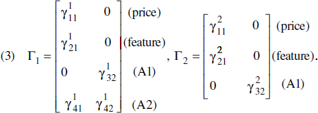
Γ_{1} = [\begin{array}{l} γ_{11}^{1} & 0 \\ γ_{21}^{1} & 0 \\ 0 & γ_{32}^{1} \\ γ_{41}^{1} & γ_{42}^{1} \end{array}] \begin{array}{l} (price) \\ (feature) \\ (A 1) \\ (A 2) \end{array}, Γ_{2} = [\begin{array}{l} γ_{11}^{2} & 0 \\ γ_{21}^{2} & 0 \\ 0 & γ_{32}^{2} \end{array}] \begin{matrix} (price) \\ (feature) \\ (A 1) \end{matrix} .

(3)

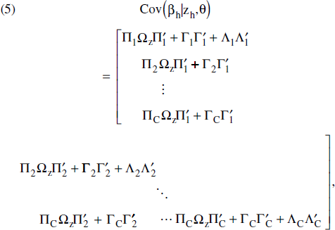
Here, Factor 1 affects price and feature sensitivities and preference for A2 in the first product category. If this factor explains a substantial amount of the overall variation in price and feature sensitivities (i.e., $γ_{11}^{1}$ , $γ_{21}^{1}$ , $γ_{11}^{2}$ , and $γ_{21}^{2}$ are large), we can interpret the first factor as a component that indicates how “marketing-mix sensitive” a household is. In particular, if $γ_{11}^{1}$ , $γ_{11}^{2}$ < 0 and $γ_{21}^{1}$ , $γ_{21}^{2}$ > 0, then households with large values of the factor have both a high price sensitivity and a high sensitivity to the feature attribute (given demographics). In addition, if $γ_{41}^{1} > 0$ , then marketing-mix-sensitive households also have high sensitivity to A2. Factor 2 affects A1 and is also correlated with A2. If this factor explains most of the overall variation in the sensitivity to A1, this may be interpreted as an A1 factor. If both $γ_{32}^{1} > 0$ and $γ_{42}^{1} > 0$ , then preferences for A1 and A2 are positively correlated.

As we discussed previously, both observable variables (the z_h) and the factors induce covariation across preferences. To determine exactly what this covariation is, we can derive the implied structure of the conditional covariance matrix:

\begin{matrix} Cov (β_{h} {|z}_{h}, θ) \\ = [\begin{matrix} Γ_{1} Γ_{1}^{'} + Λ_{1} Λ_{1}^{'} \\ Γ_{2} Γ_{1}^{'} & Γ_{2} Γ_{2}^{'} + Λ_{2} Λ_{2}^{'} \\ ⋮ & ⋱ \\ Γ_{C} Γ_{1}^{'} & Γ_{C} Γ_{2}^{'} & \dots & Γ_{C} Γ_{C}^{'} + Λ_{C} Λ_{C}^{'} \end{matrix}] \end{matrix}

(4)

This matrix measures the covariation induced by the factors. To determine how much of the correlation is driven by demographic information versus the factors, we can also compute the unconditional covariance matrix:

\begin{matrix} Cov (β_{h} | z_{h}, θ) \\ = [\begin{matrix} \prod_{1} Ω_{z} \prod_{1}^{'} + Γ_{1} Γ_{1}^{'} + Λ_{1} Λ_{1}^{'} \\ \prod_{2} Ω_{z} \prod_{1}^{'} + Γ_{2} Γ_{1}^{'} \\ ⋮ \\ \prod_{C} Ω_{z} \prod_{1}^{'} + Γ_{C} Γ_{1}^{'} \end{matrix} \\ \begin{matrix} \prod_{2} Ω_{z} \prod_{2}^{'} + Γ_{2} Γ_{2}^{'} + Λ_{2} Λ_{2}^{'} \\ ⋱ \\ \prod_{C} Ω_{z} \prod_{2}^{'} + Γ_{C} Γ_{2}^{'} & \dots & \prod_{C} Ω_{z} \prod_{C}^{'} + Γ_{C} Γ_{C}^{'} + Λ_{C} Λ_{C}^{'} \end{matrix}], \end{matrix}

(5)

where Ω_z is the covariance matrix of the demographic data: Cov(z_h) = Ω_z. In our subsequent empirical applications, we find that the covariances in Equation 5 change only marginally from the covariances in Equation 4, so we focus on Equation 4 and the household-level estimates.³

Ainslie and Rossi (1998) report a similar finding.

We assume that the error term in Equation 1, ε_h,j,c,t, follows an extreme value distribution, leading to the well-known logit model (McFadden 1981). For inference, we use a hierarchical Bayesian approach. In particular, we use a Markov chain Monte Carlo procedure to simulate the posterior distribution of the model parameters and to compute household level estimates of preferences. As Allenby and Rossi (1999) discuss, Bayesian procedures are well suited for these models, especially when making inferences at the individual level. The Gibbs sampler for this model is relatively straightforward. Gelfand and Smith (1990) provide a general overview of these methods; McCulloch and Rossi (1994) and Rossi, McCulloch, and Allenby (1996) discuss multinomial probit models; and Allenby and Lenk (1994) discuss models in which the error term follows an extreme value distribution. The estimation of multicategory models, such as the one we described previously, is an extension of the basic sampler that is laid out in these articles. A computationally intensive step involves drawing from the posterior of each person's parameter space, which requires the use of the Metropolis–Hastings (M–H) algorithm. In our initial estimation trials, a standard M–H algorithm resulted in an inefficient sampler.⁴ Thus, we use the Hybrid Monte Carlo algorithm that Duane and colleagues (1987) originally developed. Duane and colleagues' key insight is to use information about the gradient of the target distribution in guiding the choice of proposed draws in an M–H-like algorithm. The algorithm gives an automated method for generating efficient proposals, thus alleviating the difficulties of finding a good proposal distribution directly. (A full description of the estimation algorithm is available on request.)

In particular, the draws of the household-level parameters and the parameters in the factor loading matrices exhibited extremely large autocorrelations.

Applications

Snack Food Categories

Data

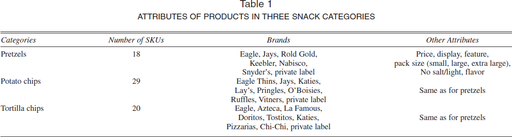
We analyze household purchasing in three snack food categories: potato chips, tortilla chips, and pretzels. These are the three largest salty snack categories in terms of per capita consumption in the United States, with market shares of 26.5%, 19.9%, and 5.7%, respectively, of a $22.5 billion market in 2002 (Snack Food and Wholesale Bakery Magazine 2003). We obtained the data from a market basket database available through Information Resources Inc. For our analysis, we included the top-selling 18 SKUs of pretzels, 29 SKUs of potato chips, and 20 SKUs of tortilla chips. The selected products capture more than 75% sales in each category. The large number of SKUs included in our analysis reflects an advantage of the attribute-based choice modeling approach (Fader and Hardie 1996). We chose a random sample of 250 households from among all households that purchased at least once in each of the three categories over a two-year period. Selected households made 1772 purchases of pretzels, 5725 purchases of potato chips, and 2430 purchases of tortilla chips. In addition to the purchase histories and the marketing environment, we also observed several demographic characteristics for these households: the size of the family, household income, an indicator for race (coded as 1 for white), age of the head of the household, and an indicator for whether the household has children. We describe each SKU with respect to the following attributes and levels (see Table 1): brand name (several levels),⁵ flavor (e.g., barbeque, spicy; characterized as yes or no), no salt/light (yes or no),⁶ and pack size (small, large, and extra large). In addition, marketing variables, such as price, display, and feature, are common across the categories.⁷

Table 1

ATTRIBUTES OF PRODUCTS IN THREE SNACK CATEGORIES

Categories	Number of SKUs	Brands	Other Attributes
Pretzels	18	Eagle, Jays, Rold Gold, Keebler, Nabisco, Snyder's, private label	Price, display, feature, pack size (small, large, extra large), No salt/light, flavor
Potato chips	29	Eagle Thins, Jays, Katies, Lay's, Pringles, O'Boisies, Ruffles, Vitners, private label	Same as for pretzels
Tortilla chips	20	Eagle, Azteca, La Famous, Doritos, Tostitos, Katies, Pizzarias, Chi-Chi, private label	Same as for pretzels

We use “effects coding” for the brand dummies to avoid having different baseline brands in the three categories. In other words, the brand intercepts are constrained to sum to zero within each category. We thank Seenu Srinivasan for this suggestion.

We combined the no-salt and light attributes because they are highly correlated. Products with no salt are recommended for low-sodium diets. They have relatively small shares in the potato chips and tortilla chips categories (approximately 7% and 3%, respectively), but they have an approximately 14% share in the pretzels category.

We explicitly do not include interactions between the marketing variables in our model to limit the number of parameters. Recent models (e.g., Van Heerde, Leeflang, and Wittink 2004) find significant interaction effects in single-category models. We recognize that our ability to find commonalities across categories may be affected by the incompleteness of the model in this regard.

Results

Using the methodology and the data we described previously, we estimated several models using different normalizations and a different number of factors. Determining the number of factors to use is a nontrivial problem in a nonlinear factor model such as ours. We used three measures to determine the number of factors: (1) in-sample and out-of-sample hit rates, (2) log marginal density of the data (we estimated this using Newton and Raftery's [1994] method), and (3) observed correlation patterns. We estimated one-, two-, three-, and four-factor versions of the model. On the basis of the hit rates, it was difficult for us to discriminate between the competing models, because we found roughly the same hit rates as we increased the number of factors (out-of-sample hit rates were approximately .51 for pretzels, .39 for potato chips, and .51 for tortilla chips, which are quite good considering the large number of alternatives). Parsimony dictates choosing the one-factor model. However, the marginal likelihood showed large increases going from one to two and from two to three factors and a smaller increase going from three to four factors.⁸ Similarly, the implied correlation matrix changed quite dramatically when we increased the number of factors from one to two and from two to three but much less when going from three to a four factors. On the basis of these metrics, we chose the four-factor model (the model comparison statistics are available on request).

The main reason for the difference between hit rates and the log marginal density is that hit rates do not reveal anything about how the model is fitting the second (and higher) moments of the data.

The model in Equation 2 explains variation in attribute preferences of households based on the five demographic characteristics Z and unobservable traits represented by the four factors ψ₁, ψ₂, ψ₃, and ψ₄. In Table 2, for each of the categories, we show the proportion of variance that each of the category-invariant components explains and U, the residual variation that is category specific and remains unexplained (denoted as “Error” in the table). The proportions in each row add up to one within each category. In each of the three categories, the household components taken together explain a substantial proportion of the variation in sensitivity to price and, to a lesser extent, display and feature, as well as a substantial proportion of preferences for flavor, no salt/light, and pack sizes. Preferences for brand names (not shown for reasons of space) are category specific to a greater degree. We also note that demographic variables explain more of the variation in the marketing-mix sensitivities than they do for other attribute preferences, particularly in the pretzels and tortilla chips categories. However, consistent with prior studies, we find that, on average, the variation that demographic variables explain is not large. The proportion of variance that each of the factors explain (the numbers are not shown separately for each factor) helps interpret the factors, a point we return to subsequently.

Table 2

VARIANCE DECOMPOSITION FOR SNACK FOOD CATEGORIES

Attribute	Pretzels			Potato Chips			Tortilla Chips
Attribute	Demographics	Factors	Error	Demographics	Factors	Error	Demographics	Factors	Error
Price	.21	.68	.12	.13	.62	.24	.21	.65	.15
Feature	.28	.29	.43	.14	.21	.66	.19	.39	.42
Display	.42	.33	.25	.17	.45	.37	.28	.20	.52
Flavor	.05	.18	.77	.14	.39	.48	.08	.70	.22
No salt/light	.07	.56	.36	.1	.7	.2	.15	.5	.36
Extra large	.16	.78	.06	.14	.76	.1	.1	.8	.06
Large	.15	.65	.2	.13	.72	.15	.14	.84	.03
Private label	.1	.39	.51	.06	.42	.52	.08	.29	.63

In Table 3, we show the estimated hierarchical regression coefficients π_c, factor loadings γ_c, and diagonal elements of A_c for the three categories. For reasons of space, we show only the estimates for attributes that are common in at least two categories. Furthermore, we do not report the estimates for the demographic variables, because only a small number of demographic effects on attribute preferences—fewer than 15% across the three categories—are found to be statistically significant. This is consistent with the variance decomposition results we discussed previously. In terms of the mean effects for the marketing-mix variables (shown in the column labeled “Constant”), we find that with one exception, the estimates have the expected signs and are statistically significant.

Table 3

HIERARCHICAL COEFFICIENTS FOR COMMON ATTRIBUTES: SNACK CATEGORIES

Attribute	Pretzel						Potato Chip						Tortilla Chip
Attribute	Constant	ψ₁	ψ₂	ψ₃	ψ₄	λ	Constant	ψ₁	ψ₂	ψ₃	ψ₄	λ	Constant	ψ₁	ψ₂	ψ₃	ψ₄	λ
Price	-2.13 (.20)	−.23 (.28)	−.69 (.30)	−.93 (.25)	.41 (.20)	.54 (.15)	-1.64 (.33)	-2.63 (.40)	−.12 (.43)	−.58 (.41)	.82 (.43)	1.78 (.27)	−.65 (.15)	−.49 (.23)	−.29 (.23)	.35 (.24)	.50 (.23)	.41 (.17)
Feature	−.32 (.22)	−.26 (.31)	.05 (.32)	−.11 (.31)	.37 (.31)	.95 (.37)	.67 (.11)	−.29 (.16)	−.02 (.16)	.02 (.14)	−.16 (.15)	.78 (.11)	.45 (.21)	−.01 (.30)	.36 (.30)	.73 (.29)	.10 (.32)	1.04 (.30)
Display	1.13 (.21)	−.11 (.28)	−.13 (.28)	.03 (.26)	−.24 (.27)	.50 (.26)	1.43 (.10)	−.28 (.15)	.35 (.15)	−.12 (.13)	.04 (.14)	.47 (.14)	1.12 (.16)	−.10 (.22)	.08 (.22)	.20 (.22)	−.05 (.22)	.79 (.23)
Eagles	1.34 (.35)	.06 (.37)	.41 (.37)	.76 (.36)	−.54 (.36)	1.46 (.35)	.83 (.24)	−.34 (.32)	.04 (.35)	1.67 (.29)	-1.14 (.33)	.38 (.20)	−.53 (.36)	−.34 (.36)	1.05 (.37)	.82 (.39)	−.91 (.37)	1.17 (.29)
Jays	.89 (.42)	.19 (.37)	−.25 (.39)	.67 (.35)	.00 (.40)	1.68 (.45)	2.23 (.14)	−.01 (.14)	−.20 (.14)	.28 (.14)	−.07 (.14)	.87 (.08)	N.A.
Katies	N.A.						-5.40 (.98)	−.24 (.74)	-2.36 (.91)	-4.10 (.78)	−.99 (.97)	.47 (.27)	-5.76 (1.23)	−.65 (.75)	-2.93 (.93)	-2.87 (.93)	.67 (.91)	.80 (.51)
Private label	-1.36 (.36)	.17 (.48)	−.64 (.52)	-1.93 (.45)	−.13 (.43)	2.51 (.29)	−.05 (.21)	−.18 (.25)	.59 (.29)	−.99 (.28)	.00	1.34 (.18)	.66 (.27)	.20 (.29)	.64 (.30)	.13 (.31)	−.49 (.30)	1.47 (.18)
Flavor	−.84 (.20)	−.38 (.30)	−.33 (.32)	−.20 (.31)	.24 (.30)	1.76 (.23)	−.74 (.11)	.19 (.18)	.53 (.16)	.27 (.20)	.63 (.18)	1.05 (.10)	.19 (.17)	−.31 (.27)	−.66 (.27)	.62 (.30)	1.24 (.27)	.90 (.18)
No salt/light	-1.13 (.29)	-1.52 (.35)	.86 (.35)	.05 (.30)	−.39 (.31)	1.46 (.30)	-1.78 (.18)	−.82 (.28)	1.46 (.23)	.00	.00	.88 (.24)	-2.42 (.53)	-1.58 (.49)	−.17 (.50)	−.21 (.51)	−.18 (.54)	1.56 (.46)
Extra large	-4.57 (.39)	−.60 (.55)	-1.72 (.57)	-1.74 (.50)	.99 (.47)	.70 (.32)	1.77 (.26)	-2.17 (.27)	.00	.00	.00	.75 (.17)	3.22 (.65)	-2.36 (.56)	-2.43 (.54)	−.82 (.78)	−.64 (.70)	.97 (.25)
Large	-3.70 (.34)	−.70 (.47)	-1.35 (.51)	-1.49 (.46)	1.01 (.45)	1.36 (.23)	2.56 (.22)	-1.45 (.24)	−.25 (.14)	−.25 (.12)	.09 (.15)	.68 (.15)	2.40 (.65)	-2.77 (.56)	-2.66 (.55)	−.54 (.81)	−.18 (.74)	.67 (.30)

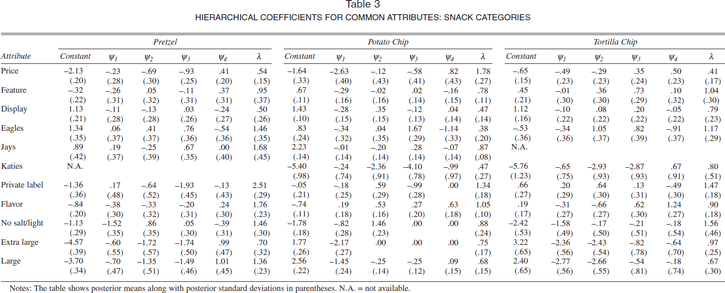
Notes: The table shows posterior means along with posterior standard deviations in parentheses. N.A. = not available.

Next, we turn to the interpretation of the factor loadings for the four factors, which we label ψ₁–ψ₄ in Table 3 for the three categories. The factor loadings represent covariances between attribute preferences and the unobserved factors. For each of the four columns, we focus on attributes with large covariances. We also take into account the variance that each of the factors explains in each attribute preference. Factor 1 captures a preference for smaller pack sizes in potato chips and tortilla chips, a preference for regular (as opposed to no salt/light) products in all three categories, and high price sensitivity in potato chips and, to a lesser degree, tortilla chips. Factor 2 captures a preference for small pack sizes in pretzels and tortilla chips and a preference for no salt/light in potato chips. Factor 3 captures a preference for a small pack size in pretzels; a preference for the Eagle brand name, which is the only brand name available in all three categories; and higher price sensitivity in pretzels. Factor 4 is correlated with a preference for flavored products in potato chips and tortilla chips and a preference for small pack size in pretzels. As we demonstrate subsequently, such an interpretation of factors could be quite useful for targeting purposes.

Correlations across categories

In Table 4, we present pairwise correlations for the three pairs of categories in marketing-variable sensitivities and selected attributes. We find that price sensitivities are positively correlated and significant in two of the three pairs of categories. The magnitudes of these correlations are similar to the average correlation of .28 that AR (1998, Table 6, p. 101) report. However, unlike AR, we do not find significant correlations in display and feature sensitivities. The significant correlations in preferences for no salt/light and flavor are positive. Preferences for the Eagle brand name of Anheuser-Busch have strong, positive correlations and, as we noted previously, load on a common factor.

Table 4

CROSS-CATEGORY CONDITIONAL CORRELATIONS IN MARKETING VARIABLE SENSITIVITIES AND SELECTED ATTRIBUTES IN THREE SNACK CATEGORIES

Attribute	P–PC	P–TORT	PC–TORT
Price	.36	.21	.45
Display	−.11	.11	−.04
Feature	−.04	−.08	.04
Flavor	−.07	.14	.19
No salt/light	.53	.40	.24
Eagles (brand)	.47	.39	.56
Private label	.22	−.12	.08

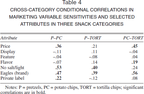
Notes: P = pretzels, PC = potato chips, TORT = tortilla chips; significant correlations are in bold.

In Table 5, we show correlations in pack-size preferences. With one exception, all the significant correlations are positive. Because the attributes represent large and extra-large pack sizes in each category, this result suggests that households are consistent in their preference for a particular pack size. Although the preference for pack size could be driven by characteristics such as household size, results on variation decomposition (Table 2) suggest that it is primarily driven by unobserved household factors (note that demographics explain only 15% of the variation, whereas the factors explain more than 75% of the variation). The unobserved factors could be, for example, how the household trades off between the benefits of quantity discounts on large pack sizes versus the product freshness of small pack sizes.

Table 5

CROSS-CATEGORY CONDITIONAL CORRELATIONS IN PACK SIZE PREFERENCE

Attribute	Pretzels (XL)	Potato Chips (XL)	Pretzels (XL)	Pretzels (L)	Potato Chips (L)
Pretzels (XL)
Potato chips (XL)	−.29
Tortilla chips (XL)	.58	−.16
Pretzels (L)	.82	−.18	.54
Potato chips (L)	.19	.41	.58	.25
Tortilla chips (L)	.60	−.15	.94	.57	.63

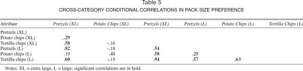
Notes: XL = extra large, L = large; significant correlations are in bold.

Finally, in Table 6, we show the correlations in preferences for the five brand names of Frito-Lay, the largest manufacturer of salty snacks. The Lay's brand is not significantly correlated with the other four. However, all other pairwise correlations are positive and significant. Because it is unlikely that consumers know that these brands have a common manufacturer, such correlations may reflect common, unobserved, manufacturer-specific attributes, such as the premium shelf space that is enjoyed by all Frito-Lay brands. The large number of significant correlations across categories in attribute preferences, beyond the marketing-mix variables, attests to the greater flexibility of our model than AR's (1998) model.

Table 6

CROSS-CATEGORY CONDITIONAL CORRELATIONS IN PREFERENCES FOR FRITO-LAY BRANDS

Attribute	Lay's	Ruffles	Rold Gold	Doritos
Lay's
Ruffles	.09
Rold Gold	.07	.34
Doritos	.21	.39	.49
Tostitos	−.01	.20	.31	.29

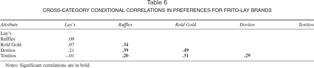
Notes: Significant correlations are in bold.

Cheese and Mayonnaise Categories

Data

The second application of our model is to household panel data provided by ACNielsen for two less closely related product categories: individually wrapped, sliced cheese and mayonnaise. The data consist of a sample of 1017 households from a large Midwestern city and span two years. Selected households make at least one purchase in each category. The sample households made a total of 8241 purchases in the cheese category and 7567 purchases in the mayonnaise category. Four demographic variables are included in the model: income, age of the household head, a dummy representing the presence of a child, and the number of members in the household. We randomly split the data into an estimation sample (917 households) and a validation sample (100 households) that we used for model comparisons.

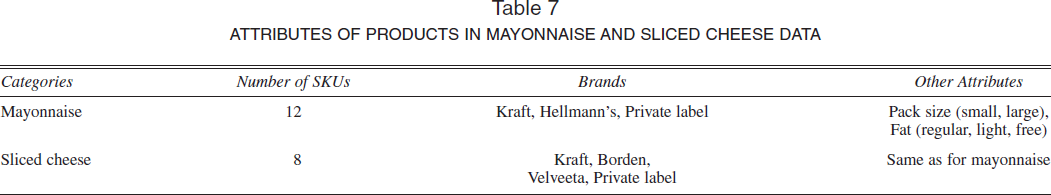
In Table 7, we show the product attributes in the two categories. In the mayonnaise category, we use data for 12 SKUs that account for more than 88% of category sales. These products represent two national brands—Kraft and Hellmann's—and private label brands. In addition to brand name, the products differ along three other attributes: size (16 oz. or 32 oz.), fat content (fat free, light, or regular), and type (mayonnaise or Miracle Whip). Thus, each product can be described by the value of the attribute vector (i.e., brand, size, fat content, and type). In the cheese category, we use purchases of 8 SKUs that account for 74% of total category sales. These products can be described in terms of four levels of the attribute brand (Kraft, Borden, Velveeta, and private label), two levels of size (12 oz. and 16 oz.), and two levels of fat content (regular or fat free). Note that some of these attribute levels—brand names (Kraft and private label), size (large and small), and fat content (regular and fat free)—are common across the two categories. Although we do not show the summary statistics because of space constraints, we should point out that the private label does not offer a better-for-you (light or fat free) product in either category; this becomes relevant in our subsequent application

Table 7

ATTRIBUTES OF PRODUCTS IN MAYONNAISE AND SLICED CHEESE DATA

Categories	Number of SKUs	Brands	Other Attributes
Mayonnaise	12	Kraft, Hellmann's, Private label	Pack size (small, large), Fat (regular, light, free)
Sliced cheese	8	Kraft, Borden, Velveeta, Private label	Same as for mayonnaise

Results

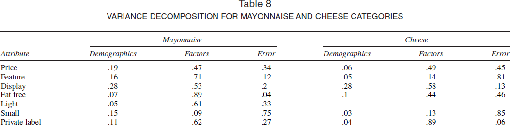
Using criteria we discussed previously in the snack foods application, we determined the appropriate number of factors to be four in these data. In Table 8, for the four-factor model, we show the proportion of variance that each of the category-invariant components explains and U, the residual variation that is category-specific and remains unexplained. We do not show the brand name attribute for reasons of space. In mayonnaise, household components taken together explain a substantial proportion of variation in the sensitivities to the three marketing-mix variables—price, display, and feature—and in preferences for private label, fat-free, and light attributes. Preference for size is category specific to a greater degree. In the cheese category, household demographics and the factors explain a substantial proportion of the variation in the following attributes: price, display, fat free, and private label. However, the variation in feature responsiveness and size preference appears to be largely category specific. As in the snack foods application, demographic variables seem to explain more of the variation in the marketing-mix sensitivities than they do for other attribute preferences. However, on average, the variation that demographic variables explain is not large.

Table 8

VARIANCE DECOMPOSITION FOR MAYONNAISE AND CHEESE CATEGORIES

Attribute	Mayonnaise			Cheese
Attribute	Demographics	Factors	Error	Demographics	Factors	Error
Price	.19	.47	.34	.06	.49	.45
Feature	.16	.71	.12	.05	.14	.81
Display	.28	.53	.20	.28	.58	.13
Fat free	.07	.89	.04	.10	.44	.46
Light	.05	.61	.33
Small	.15	.09	.75	.03	.13	.85
Private label	.11	.62	.27	.04	.89	.06

In Table 9, we show the estimated hierarchical regression coefficients π_c, factor loadings γ_c, and diagonal elements of A_c for the mayonnaise and cheese categories. Although we do not report the demographic estimates because of space constraints, we found some notable similarities in the demographic patterns across the two categories. For example, in both categories, preferences for low-fat attributes are positively related to income and negatively related to household size. Similarly, in the mayonnaise category, the private label is preferred by lower-income consumers, older consumers, and larger households. In the cheese category, the private label is preferred by older consumers, larger households, and households without young children, though the effect of income is not statistically significant. The signs of such demographic effects are consistent with conventional wisdom about consumers of private labels. There are also differences in the effects of demographics on attribute preferences across categories. For example, we find that older consumers strongly preferred the Kraft brand in the mayonnaise category, but age does not explain Kraft preferences in the cheese category.

Table 9

HIERARCHICAL COEFFICIENTS: MAYONNAISE AND CHEESE CATEGORIES

Attribute	Mayonnaise						Cheese
Attribute	Constant	ψ₁	ψ₂	ψ₃	ψ₄	λ	Constant	ψ₁	ψ₂	ψ₃	ψ₄	λ
Price	-3.82 (.38)	.54 (.40)	.28 (.53)	1.17 (.49)	.00 N.A.	1.24 (.56)	-5.37 (.31)	.15 (.29)	1.22 (.43)	.60 (.30)	1.84 (.34)	2.25 (.40)
Feature	.54 (.17)	−.07 (.17)	−.38 (.18)	.09 (.19)	−.62 (.16)	.31 (.15)	.96 (.14)	.05 (.12)	.03 (.14)	−.13 (.15)	−.31 (.14)	1.05 (.14)
Display	1.18 (.29)	−.23 (.28)	.29 (.31)	−.29 (.29)	−.42 (.28)	.46 (.25)	−.06 (.44)	.47 (.35)	.39 (.42)	−.14 (.45)	.53 (.39)	.47 (.28)
Kraft	1.27 (.14)	−.45 (.14)	.71 (.14)	−.07 (.11)	−.18 (.10)	1.14 (.09)	1.77 (.12)	.02 (.10)	.43 (.13)	−.32 (.20)	−.75 (.12)	.78 (.07)
Private	-3.43 (.25)	1.12 (.26)	-1.78 (.26)	.00 N.A.	.00 N.A.	1.37 (.23)	.25 (.16)	.40 (.14)	−.31 (.25)	-1.32 (.20)	.98 (.27)	.41 (.18)
Fat free	-3.47 (.39)	4.09 (.34)	.00 N.A.	.00 N.A.	.00 N.A.	.74 (.40)	-3.16 (.42)	2.88 (.31)	.74 (.40)	.35 (.44)	.70 (.41)	3.24 (.34)
Light	-1.98 (.26)	3.19 (.26)	−.08 (.26)	.23 (.24)	.01 (.22)	2.37 (.21)				N.A.
Mayonnaise	−.55 (.24)	.77 (.22)	-1.55 (.30)	.28 (.31)	−.38 (.33)	3.30 (.34)				N.A.
Small	-2.99 (.31)	−.21 (.24)	.16 (.32)	−.08 (.29)	.72 (.24)	2.64 (.21)	1.23 (.10)	.00 (.10)	−.19 (.11)	.18 (.13)	−.20 (.12)	1.04 (.08)
Velveeta			N.A.				-1.91 (.28)	−.30 (.22)	−.33 (.32)	2.15 (.32)	.86 (.41)	.39 (.20)

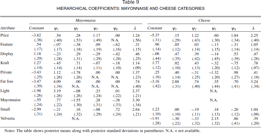
Notes: The table shows posterior means along with posterior standard deviations in parentheses. N.A. = not available.

Next, we turn to the interpretation of the factor loadings for the four factors ψ₁–ψ₄ in Table 9 for the two categories. The factor loadings represent covariances between attribute preferences and the unobserved factors, and patterns of large covariances help interpret the factors. Although we do not show the variance that each factor in each attribute explains, we can provide this information on request. Factor 1 loads strongly on the fat-free and light attributes in the mayonnaise category and on the light attribute in the cheese category. Furthermore, this factor explains a high fraction of the variance in the fat-free and light attributes in the two categories. Thus, we label this factor “diet preference.” Factors 2, 3, and 4 are not as interpretable. Factor 2 is restricted largely to the mayonnaise category and seems to reflect a preference for Kraft, which is the large national brand; a negative preference for the private label; and a preference for Miracle Whip (see the negative loading on mayonnaise). Notably, Factor 2 in the cheese category reflects a low-price sensitivity (positive loading on price), which is consistent with national brand preference. Factor 3 reflects a positive preference for Velveeta cheese, which is Kraft Foods' premium priced cheese; a negative preference for the private label cheeses; and a low-price sensitivity in the mayonnaise category. Factor 4 is limited largely to the cheese category, and it loads negatively on Kraft and positively on private label and reflects low-price sensitivity.

We chose to impose specific zero restrictions in the model to facilitate the emergence of a “diet preference” factor. However, we kept in mind the kinds of predictive applications that we demonstrate subsequently. Other application settings might require the factors to be interpreted differently. In that case, we could explore other orthogonal rotations by imposing the requisite zero restrictions.

Correlations across categories

Table 10 contains the cross-category correlations that common demographic variables and unobserved factors induced. Overall, there are many nonzero correlations in the table, so a model that assumes independence between preferences in the cheese and mayonnaise categories would be misspecified. Focusing on the correlation between related attributes in the two categories, we find strongly significant, positive correlations between the fat-free and light attributes in mayonnaise and the fat-free attribute in cheese. This finding lends support to the idea of preference for low fat as an intrinsic household trait, as the high loading of Factor 1 on the two better-for-you attributes suggests. We also observe that private label buyers in each category prefer fat-free and light attributes in the other category, whereas (as we noted previously) currently the private label product line does not include any better-for-you products. This suggests new product opportunities for private labels (see our subsequent application). A preference for the Kraft brand name is positively correlated across categories, indicating the possible existence of a cross-category segment of Kraft lovers, an important element of the brand equity of Kraft. There appears to be a segment of consumers who prefer to buy private labels in both categories, a finding that is especially relevant for retailers. Russell and Kamakura (2001) also report that cross-category preferences for private label brands in four paper categories are positively correlated. Furthermore, the size attribute is uncorrelated across categories. This is in contrast with the high correlation in preference for pack sizes in the three snack categories. For marketing-mix sensitivities, we find lower correlations than those that AR (1998) report, especially for feature and display sensitivity.⁹

Table 10

INDUCED CONDITIONAL CORRELATION MATRIX BETWEEN CATEGORY 1 (MAYONNAISE) AND CATEGORY 2 (CHEESE)

Cheese Attributes	Mayonnaise Attributes
Cheese Attributes	Price	Feature	Display	Kraft	Private	Fat Free	Light	Mayonnais	Small
Price	.19 (.13)	−.56 (.11)	−.20 (.22)	.09 (.08)	−.24 (.09)	.04 (.09)	.04 (.07)	−.18 (.06)	.16 (.07)
Feature	−.05 (.10)	.18 (.12)	.15 (.13)	.04 (.07)	.00 (.10)	.04 (.10)	.03 (.08)	.02 (.06)	−.07 (.05)
Display	.09 (.28)	−.50 (.26)	−.15 (.34)	−.01 (.20)	−.05 (.27)	.37 (.26)	.29 (.21)	−.10 (.16)	.11 (.12)
Kraft	−.07 (.13)	.28 (.15)	.45 (.18)	.26 (.07)	−.23 (.08)	.02 (.08)	.00 (.06)	−.10 (.06)	−.14 (.07)
Private	−.40 (.16)	−.41 (.15)	−.11 (.27)	−.18 (.08)	.21 (.08)	.21 (.08)	.14 (.06)	.00 (.06)	.13 (.08)
Velveeta	.45 (.18)	−.11 (.19)	−.44 (.26)	−.12 (.08)	.04 (.09)	−.12 (.09)	−.04 (.07)	.06 (.07)	.08 (.09)
Fat free	.24 (.14)	−.23 (.15)	−.19 (.20)	−.14 (.07)	.17 (.08)	.62 (.05)	.51 (.04)	.05 (.05)	.00 (.06)
Small	.06 (.10)	.23 (.10)	−.02 (.13)	−.07 (.06)	.12 (.07)	.00 (.08)	.01 (.07)	.10 (.05)	−.06 (.04)

Notes: The table shows posterior means along with posterior standard deviations in parentheses.

When we used the information contained in households' purchase histories (i.e., when we examined household-level estimates), we obtained correlation estimates that were much closer to those of AR (1998) for price and feature sensitivities, which we discuss subsequently.

Household-level estimates of preferences (β_mayonnaise,h, β_cheese,h) are readily available from our Markov chain Monte Carlo algorithm. In Figure 1, we plot the estimates for the attributes that are common to both categories. These plots mirror the results of the cross-category correlations that appear in Table 10. There are strong correlations across categories in preferences for fat-free and light attributes, the private label attribute, and the Kraft attribute. It is also worth noting that the correlations for price and feature sensitivity are substantial (at the household level, the correlation between price sensitivities is .31 and is .47 for feature sensitivities).

Figure 1

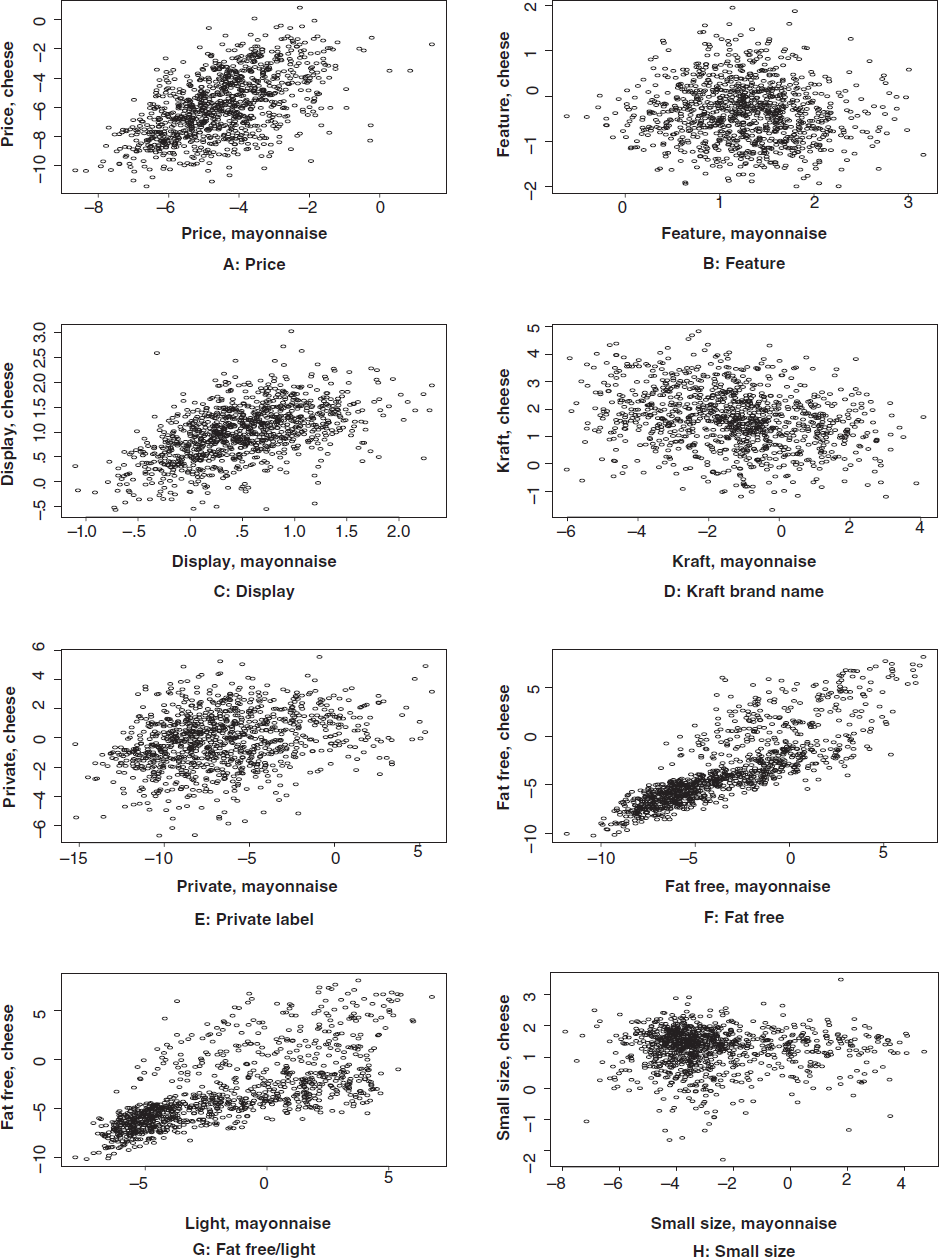
ACROSS CATEGORY CORRELATIONS OF ESTIMATED HOUSEHOLD LEVEL PREFERENCES FOR COMMON ATTRIBUTES

Summary of the Main Findings

To summarize, we have presented two applications of our model. The first compares household purchase data for a set of three closely related snack food categories (pretzels, potato chips, and tortilla chips) that are purchased for similar consumption needs. In these categories, we find significant correlations in preferences for product attributes such as brand names, pack sizes, and no salt/light, as well as price sensitivities. The second application explores the robustness of the multicategory model; we apply this model to two food categories (sliced cheese and mayonnaise) that are purchased for unrelated consumption needs and have fewer common attributes. In this application, we find significant correlations in preferences for attributes such as fat free and private label, as well as marketing-mix sensitivities. These findings lend support to the idea that certain unobservable household characteristics or “traits” are common across product categories. Such high correlations in product attribute preferences also create opportunities for cross-category targeting, which we discuss subsequently.

Cross-Category Targeting Applications

Our multicategory model has the potential to elicit information about a household's preferences for “new” product categories—that is, categories in which no purchase information for the household is available. In the context of packaged goods categories, it is well documented that relatively little can be learned about a household's preferences from household demographics, and our previous findings confirm this. For a single category, Rossi, McCulloch, and Allenby (1996) show that though observable household characteristics contain little information about preferences, prior purchase behavior in the category is informative about brand preferences and marketing-mix sensitivities. Thus, for the design of targeting schemes, prior purchases contain valuable information.

From a manufacturer's perspective, the problem of eliciting households' preferences often involves many different product categories. As we noted previously, many large packaged goods manufacturers offer products in several categories (e.g., Kraft Foods, General Mills, Procter & Gamble). If it is the manufacturer's goal to predict a household's preferences in all relevant categories through the use of prior purchases, a large database of shopping information in all categories is necessary. This is costly and can be a complicated matter to implement. Such problems raise the possibility of using purchase information in a few select categories to infer a household's preferences for products in many other categories. The approach is even more appealing when predicting the likely targets for a new product. The introduction of a new product represents the single most expensive investment for consumer product companies, with an estimated 30,000 new products introduced in 2000 (ACNielsen 2001). It is alarming that 93% of these new products failed, with total failure costs exceeding $20 billion. Furthermore, most retailers have narrowed the evaluation period for a new product to between six and nine months. Thus, it is imperative for manufacturers to target their new products to most likely buyers, especially in the initial phases of the product launch.

The appeal of the proposed model in the targeting of new products depends on how much can be learned about consumers' preferences for a new product by using the demographic and purchase history information from existing categories. In general, it is expected that both a larger number of shared attributes across categories and a higher correlation in preferences for these common attributes lead to higher information transfer across categories. However, a single, but important, attribute might be quite informative. For example, if soy is an attribute that appeals to certain types of households, it may be possible to learn about the likely targets for a new Kellogg's soy protein cereal by using information on other soy-based products. Similarly, attributes such as private label, diet, or organic might be quite informative.

We illustrate the potential benefits of our multicategory brand choice model in two different cross-category targeting applications. In both situations, the goal is to score a group of potential customers, called the “target group,” on the basis of their buying preferences in a target category without observing their purchases in this category. In both situations, we have access to data on the purchases of the target group in other categories that share common attributes with the target category. The difference between the two situations is as follows: In the first situation, we also have available the complete purchase data of a reference group of customers—that is, their purchases in both the target category and other categories. (We borrow the terminology of target group and reference group from Iyengar, Ansari, and Gupta's [2003] work.) Thus, the prediction problem is to target customers in existing categories. In the second situation, no such reference group is available. Thus, predictions in the target category must be based entirely on purchase data from other product categories—a case of targeting customers in new categories.

Targeting Customers in Existing Categories

Previously, we presented estimates of the multicategory model based on purchase data of an estimation sample of 917 households in the mayonnaise and sliced cheese categories. We now consider the problem of choosing targets for a new hypothetical cheese product—a low-fat cheese offered as a private label in the small pack size. Recall that our empirical results suggest high potential for such a new product. A list of potential customers (the target group) is available, but we do not know their purchase history in the cheese category. Our goal is to rank order these customers in terms of their predicted choice probability for the new cheese product.

We take the 100 households in the holdout sample to be representative of the target group. For computing the predicted choice probabilities, we use the estimated model and data that are available for households in the target group under three alternative information sets:

I₁: the information set that consists of only the demographic variables,

I₂: I₁ plus each household's purchase history in the mayonnaise category, and

I₃: I₂ plus each household's purchase history in the cheese category.

Note that I₁ ⊂ I₂ ⊂ I₃. Because I₃ is the most information we might have in real life, we take the estimated rank ordering under I₃ to be the “true” rank ordering of the target households.

In Figure 2, we show the scatterplot of predicted ranks for the 100 households under I₁ on the x-axis and under I₃ on the y-axis. The 45-degree line represents the “true” ranks, so the closer the circles are to the 45-degree line, the smaller is the error in predicted ranks compared with the truth. We also show the line of best fit to the predicted ranks. As is evident, the predictions are not very good. In Figure 3, we show the results for predicted ranks under I₂ on the x-axis and under I₃ on the y-axis. The line of best fit now lies much closer to the 45-degree line, indicating that the information contained in purchase histories of mayonnaise is valuable for rank ordering target consumers in the cheese category on the basis of their likelihood to buy a new product concept.

Figure 2

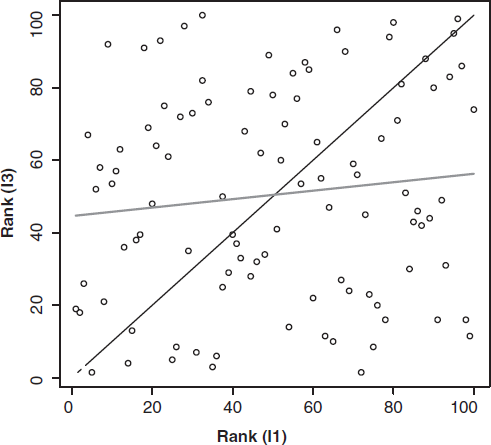
PREDICTED RANKINGS USING INFORMATION SETS I3 AND I1

Figure 3

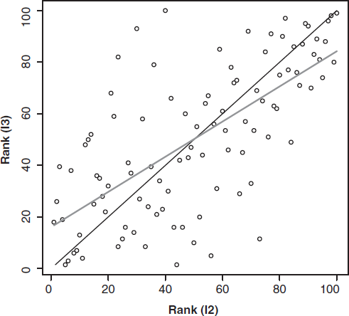
PREDICTED RANKINGS USING INFORMATION SETS I3 AND I2

Targeting Customers in New Categories

For this application, we use the multicategory model estimates from the three snack categories. Our goal is to assess the extent to which the estimated preferences predict households' purchase behavior in an entirely new category that shares some common attributes with the three snack categories. Recall that one of the attributes in the snack foods categories is no salt/light and that Factors 1 and 2 were correlated with preference for this attribute. If these factors capture an underlying household trait of “healthy eating,” we expect to find households with high factor values to be more likely to choose healthful products in other categories.

We also observed 244 of the 250 households used for estimating the model for the snack categories to buy in the ice-cream category during the two-year period. An important attribute in the ice-cream category is diet/light; light ice creams account for 22% of the market in our data. To assess the predictive ability of the model estimated on the snack data, we classify the 244 sample households into the four quartiles based on their estimated Factor 1 scores and into the four quartiles based on their estimated Factor 2 scores (we normalized the factors so that a higher factor score leads to a higher preference for the diet/light attribute for the estimation categories). A cross-tabulation of the two classifications yields a 16-cell matrix. Within each cell, we compute the average market share of light ice cream. In Figure 4, we plot these data. The figure shows that households with high market shares of light ice cream are easily identified on the basis of their joint Factor 1 and Factor 2 scores. These households have large values of Factors 1 and 2. We believe that this simple tool can be useful for new product managers.

Figure 4

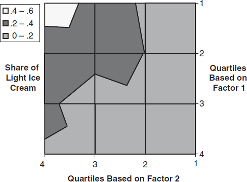
CONTOUR PLOT OF SHARE OF LIGHT ICE CREAM BY FACTORS 1 AND 2

To further examine the usefulness of the factor estimates for targeting consumers of light ice cream, for each factor we compute the cumulative percentage of light-ice-cream buyers that each quintile captured. In Figure 5, we show the resulting gains charts. The 45-degree line represents the performance if the targeting is random. Gains due to information from the factor estimates are reflected in the extent to which the line lies above the 45-degree line. For example, the chart shows that 20% of the target group based on the highest values of Factor 1 includes 41.4% of light-icecream buyers. In contrast, 20% of a randomly picked target group would include only 20% of light-ice-cream buyers. Again, Figure 5 shows that the estimated factor values from the snack data provide significant value in targeting light-ice-cream buyers.

Figure 5

GAINS CHART FOR TARGETING LIGHT-ICE-CREAM BUYERS

Conclusions and Further Research

Emerging literature in marketing recognizes and models the dependence among consumers' brand choices across multiple categories. This article contributes to the literature by offering a model of dependence based on correlated preferences for attributes that are shared by categories. Our model decomposes the intrinsic preference for each product in each category into preferences for elemental attributes or characteristics, some of which are common across categories. Therefore, we allow correlated preferences for the elemental attributes to determine similarities in choice behavior across categories. Furthermore, we project the unobserved component of preferences for attributes and sensitivities to marketing-mix variables to a lower dimensional space of unobserved factors. The factors are interpretable as unobservable household traits that drive similarity in choice behaviors across categories. Because the factors transcend categories, we can use household-specific factor estimates derived from purchasing in existing categories to predict preferences for attributes in new categories. In our empirical application of consumer purchases in both closely related and less-related food categories, we find high correlations in preferences for product attributes across categories. In two applications, we demonstrate that these high correlations in product attribute preferences across categories imply that (1) the model estimates can be used to forecast preferences for an attribute in a new category and (2) potential targets for a new product in an existing category can be rank ordered on the basis of their probability of choice.

There are several caveats to our study and directions for further research. We were limited by the available set of product categories. It would be worthwhile to apply the model to a large set of diverse categories that include apparently different attributes, such as organic, trans fat, low carb, environment friendly, recycled, and so forth. We believe that the factor structure in our model might reveal that households' preferences for these attributes are correlated with a small number of underlying factors. For grocery products, frequent-shopper databases that record household purchase behavior across all categories could be useful. In industries such as consumer durables or services, detailed behavioral data may not be available; thus, approaches based on stated intentions or preferences might be more suitable. For example, conjoint analysis has typically been used to measure attribute preferences within categories, but there may be an opportunity to extend the approach to measure the correlation of preferences across categories.

Another issue that we believe is worth exploring is the selection of an informative set of categories for the prediction of consumer preferences in entirely new categories. Intuitively, the problem is that of learning about consumer traits from their purchases in existing categories—learning that can be transferred to other categories. What characteristics of categories make them informative about consumers' attribute preferences and to what extent can they be used as a basis for market segmentation in the existing products and in forecasting demand for new products?

Our modeling approach could also be extended to incorporate purchase incidences in a multicategory setting (e.g., Deepak, Ansari, and Gupta 2002; Manchanda, Ansari, and Gupta 1999). Similarly, in the current applications, we used the factor structure primarily as a tool to model dependence in preferences. As a result, we did not focus heavily on the interpretation and labeling of factors. In other applications, it might be advantageous to impose other restrictions on the loadings matrix so as to facilitate interpretations of the factors. Finally, it would be fruitful to extend the current static model to dynamic settings. This would be relevant particularly in the context of the introduction of new attributes or attribute levels into existing categories and the resultant change in consumers' preference structure.

References

ACNielsen (2001), Consumer and Market Trends Report, (September). Schaumburg, IL: ACNielsen.

Ainslie

, and Rossi

(1998), “Similarities in Choice Behavior Across Multiple Categories,” Marketing Science, 17(2), 91–106.

Allenby

, and Lenk

(1994), “Modeling Household Purchase Behavior with Logistic Normal Regression,” Journal of the American Statistical Association, 89(December), 1218–31.

Allenby

, and Rossi

P.E.

(1999), “Marketing Models of Consumer Heterogeneity,” Journal of Econometrics, 89(1-2), 57–78.

Anderson

T.W.

, and Rubin

(1956), “Statistical Inference in Factor Analysis,” in Proceedings of the Third Berkeley Symposium on Mathematical Statistics and Probability, Vol. 5, Neymann

, ed. Berkeley: University of California Press, 111–50.

Bell

, Chiang

, and Padmanabhan

(1999), “The Decomposition of Promotional Response: An Empirical Generalization,” Marketing Science, 18(4), 504–526.

Blattberg

, Peacock

, and Sen

(1976), “Purchasing Strategies Across Product Categories,” Journal of Consumer Research, 3(3), 143–54.

Chintagunta

(1994), “Heterogeneous Logit Model Implications for Brand Positioning,” Journal of Marketing Research, 31(May), 304–311.

Chintagunta

, and Haldar

(1998), “Investigating Purchase Timing Behavior in Two Related Product Categories,” Journal of Marketing Research, 35(February), 43–53.

10.

Deepak

, Ansari

, and Gupta

(2002), “Investigating Consumer Price Sensitivities Across Categories,” working paper, arketing Department, University of Iowa.

11.

Dhar

, and Simonson

(1999), “Making Complementary Choices in Consumption Episodes: Highlighting Versus Balancing,” Journal of Marketing Research, 36(February), 29–44.

12.

Duane

, Kennedy

A.D.

, Pendleton

B.J.

, and Roweth

(1987), “Hybrid Monte Carlo,” Physics Letters B, 195(2), 216–22.

13.

Elrod

(1988), “Choice Map: Inferring a Product Market Map from Panel Data,” Marketing Science, 7(1), 21–40.

14.

Elrod

, and Keane

M.P.

(1995), “A Factor-Analytic Probit Model for Representing the Market Structure in Panel Data,” Journal of Marketing Research, 32(February), 1–16.

15.

Erdem

(1998), “An Empirical Analysis of Umbrella Branding,” Journal of Marketing Research, 35(August), 339–51.

16.

Erdem

, and Sun

(2002), “An Empirical Investigation of the Spillover Effects of Advertising and Sales Promotions in Umbrella Branding,” Journal of Marketing Research, 39(November), 1–16.

17.

Erdem

, and Winer

(1999), “Econometric Modeling of Competition: A Multi-Category Choice-Based Mapping Approach,” Journal of Econometrics, 89(1-2), 159–75.

18.

Fader

, and Hardie

(1996), “Modeling Consumer Choice Among SKUs,” Journal of Marketing Research, 33(November), 442–52.

19.

Gelfand

, and Smith

(1990), “Sampling-Based Approaches to Calculating Marginal Densities,” Journal of the American Statistical Association, 85(410), 398–409.

20.

Gupta

, and Chintagunta

(1994), “On Using Demographic Variables to Determine Segment Membership in Logit Mixture Models,” Journal of Marketing Research, 31(February), 128–36.

21.

Iyengar

, Ansari

, and Gupta

(2003), “Leveraging Information Across Categories,” Quantitative Marketing and Economics, 1(4), 425–65.

22.

Kim

, Srinivasan

, and Wilcox

(1999), “Identifying Price Sensitive Consumers: The Relative Merits of Demographic Vs. Purchase Pattern Information,” Journal of Retailing, 75(2), 173–93.

23.

Manchanda

, Ansari

, and Gupta

(1999), “The ‘Shopping Basket’: A Model of Multicategory Purchase Incidence Decisions,” Marketing Science, 18(2), 95–114.

24.

McCulloch

, and Rossi

(1994), “An Exact Likelihood Approach to Analysis of the MNP Model,” Journal of Econometrics, 64(1-2), 207–240.

25.

McFadden

(1981), “Econometric Models of Probabilistic Choice,” in Structural Analysis of Discrete Data with Econometric Applications, Manski

, and McFadden

, eds. Cambridge, MA: MIT Press.

26.

Newton

, and Raftery

(1994), “Approximate Bayesian Inference with the Weighted Likelihood Bootstrap,” Journal of the Royal Statistical Society, Series B, 56(1), 3–48.

27.

Park

C.S.

, and Srinivasan

(1994), “A Survey-Based Method for Measuring and Understanding Brand Equity and Its Extendability,” Journal of Marketing Research, 31(May), 271–88.

28.

Rogers

(2001), “Structural Change in U.S. Food Manufacturing, 1958-1997,” Agribusiness: An International Journal, 17(1), 3–32.

29.

Rossi

, McCulloch

, and Allenby

(1996), “On the Value of Household Purchase History Information in Target Marketing,” Marketing Science, 15(4), 321–40.

30.

Russell

G.J.

, and Kamakura

W.A.

(2001), “Modeling Multiple Category Brand Preference with Household Basket Data,” Journal of Retailing, 73(4), 439–61.

31.

Seetharaman

P.B.

, Ainslie

, and Chintagunta

(1999), “Investigating Household State Dependence Effects Across Categories,” Journal of Marketing Research, 36(November), 488–500.

32.

Snack Food and Wholesale Bakery Magazine (2003), “State of the Industry Report,” (July 1).

33.

Van Heerde

H.J.

, Gupta

, and Wittink

D.R.

(2003), “Is 75% of the Sales Promotion Due to Brand Switching? No, Only 33% Is,” Journal of Marketing Research, 40(November), 481–91.

34.

Van Heerde

H.J.

, Leeflang

P.S.H.

, and Wittink

D.R.

(2004), “Decomposing the Sales Promotion Bump with Store Data,” Marketing Science, 23(3), 317–34.