The Effect of Customer Satisfaction on Consumer Spending Growth

Abstract

Predicting aggregate consumer spending is vitally important to marketing planning, yet traditional economic theory holds that predicting changes in aggregate consumer spending is not possible. Previous attempts to predict consumer spending growth using standard macroeconomic predictor variables have met with little success. The authors show that the lagged change in customer satisfaction, which contributes to future demand, has a significant impact on spending growth. However, this impact is moderated by increases in consumers’ debt service ratio, a key budget constraint that affects consumers’ ability to spend. Using an asymmetric growth model, more than 23% of the variation in the one-quarter-ahead spending growth is explained, which represents a notable improvement over prior specifications.

Keywords

customer satisfaction consumer spending consumer confidence forecasting

The economic importance of consumer spending growth can hardly be overestimated. In the U.S. national accounts, consumer spending represents more than 70% of gross domestic product (GDP). Therefore, it should come as no surprise that changes in consumer spending are closely monitored by public policy makers and marketing managers alike. Indeed, even fairly small changes in consumer spending have profound implications for the health of the economy as a whole and for numerous companies and industries. Neither the government nor individual firms want consumer spending to go down, and economic policy is designed to balance current spending with savings/investments to enable spending in the future. The Federal Reserve has repeatedly cut interest rates to make borrowing (and subsequent spending) easier (Chicago Tribune 2008; Lahart 2003), while many durable goods manufacturers have switched to 0% financing to keep their sales levels up (Pauwels et al. 2004).

Reports of declining consumer expenditures cause managers to adapt their marketing strategy along multiple dimensions. Increased nervousness about future consumer spending makes organizations reluctant to make long-term commitments to brand advertising, switching instead to tactics they know will drive short-term sales (Grande 2006). Retailers adjust not only their pricing strategy but also their assortment composition in the wake of reduced consumer spending. For example, amid a gloomy outlook for the U.S. economy, Wal-Mart cut prices of thousands of back-to-school items in summer 2007 and discontinued several higher-priced lines (Guerrera, Weitzman, and Kim 2007). As consumer spending improves, managers make the reverse adjustments. As a case in point, increased consumer spending in summer 2004 caused shoe retailers not only to increase their marketing expenditures but also to add more high-end products to their assortment (Gray 2004).

Therefore, it is critical to anticipate movements in consumer spending. However, the problem is that consumer spending growth is difficult to predict. According to the well-known permanent-income (Friedman 1957) and life-cycle (Modigliani 1971) models of consumption, consumption expenditures follow a random-walk process (for a formal treatment, see Hall 1978). This implies that future consumption is a function only of current consumption and that all other information is irrelevant. An empirically testable implication of this contention is that consumption should be “unrelated to any economic variable that is observed in earlier periods” (Hall 1978, p. 972). Indeed, current spending by households is assumed to reflect all available relevant information, making future changes in spending de facto unpredictable. Similar reasoning underlies many tests of the efficient market hypothesis in finance (see, e.g., Cornell 1977; Fama 1970).

Still, prior empirical work has found several, albeit weak, correlates of spending growth. For example, Carroll, Fuhrer, and Wilcox (1994) find that lagged values of the Index of Consumer Sentiment (ICS) explained approximately 14% of the one-quarter-ahead variation in the growth of total real personal consumption expenditures; Murphy (2000) explains approximately 8% on the basis of lagged debt service ratios (DSRs); and Case, Quigley, and Shiller (2001) explain approximately 8% (in combination with income, but using contemporaneous analyses) of the variation in consumer spending on the basis of changes in housing wealth. Ludvigson (2004) concludes that sentiment and confidence indexes add only modest information to spending forecasts. On the one hand, these results are impressive because they empirically seem to refute a key implication of the life-cycle/permanent-income models of consumption. On the other hand, from the point of view of an applied economic forecasting, they are of limited value.

Several researchers have taken the failure of the life-cycle/permanent-income models in aggregate data as established and have tried to identify the underlying reasons for this failure. Explanations that have been put forward include consumer myopia, consumer liquidity constraints, and credit-induced habit modifications (see, e.g., Messinis, Henry, and Olekalns 2002; Shea 1995). These studies have certain implications with respect to how consumers react to predictable improvements versus deteriorations of their financial condition. As a result, various asymmetric consumption models have been proposed. Many of them provide empirical support for the notion that consumers react differently to an improvement than to a deterioration in their financial condition (see, e.g., Carruth and Dickerson 2003; Shea 1995). For example, Deleersnyder and colleagues (2004) and Lamey and colleagues (2007) find an asymmetric consumer response across economic expansions and contractions. Rao and Bharadwaj (2008) make a case for distinguishing between up and down states of the economy.

However, to the best of our knowledge, no prior specification (neither symmetric nor asymmetric) has considered the role of marketing in predicting future consumer spending growth. Still, the marketing discipline, as a bridge between production and consumption, is at the center of the issue and might well contribute to the prediction of aggregate consumer spending. In this study, we view the role of lagged gross consumption utility (i.e., customer satisfaction) as a predictor of discretionary spending growth. We examine the impact of customer satisfaction not only because it has been found to be the most commonly used perceptual metric by researchers and managers (Gupta and Zeithaml 2006; Keiningham et al. 2007; Zeithaml et al. 2006) but also because it is generic and universally applicable across all products and services and because it comes with a theoretical rationale.

Discretionary expenditures are usually defined as personal consumer expenditures less food, medical care, and housing. As Hall (1978, p. 979) indicates, “all of the theoretical foundations of the aggregate consumption function apply to individual categories of consumption as well,” and Katona's (1975, 1979) distinction between “willingness” and “ability” to pay is also phrased in terms of discretionary consumer expenditures (DCEs). In contrast, nondiscretionary expenditures are much more stable and do not fluctuate much in the aggregate, regardless of economic conditions or changes in customer satisfaction (Lamey et al. 2007).

We find that lagged changes in customer satisfaction, which contribute to consumers’ willingness to spend, have a significant impact on spending growth. This impact is also moderated by household DSR, which is a constraint on consumers’ ability to spend. We introduce a simple asymmetric growth model that explains a substantial part of future spending growth. These findings represent a notable improvement over earlier attempts to forecast spending growth and illustrate the importance of marketing metrics to macroeconomic concerns of relevance to business planning and adaption.

Customer Satisfaction and Expenditure Growth

Customer satisfaction has been shown to affect choice and purchase behavior at the individual consumer level (e.g., Homburg, Koschate, and Hoyer 2005; Keiningham, Perkins-Munn, and Evans 2003; Rust and Zahorik 1993; for a comprehensive review, see Oliver 1997). In this article, we examine whether a similar relationship can be found when both satisfaction and spending are aggregated across the U.S. population. Prior research has already linked aggregate satisfaction scores to aggregate market share (Anderson, Fornell, and Lehmann 1994), shareholder value (Anderson, Fornell, and Mazvancheryl 2004; Gruca and Rego 2005), long-term profitability (Anderson, Fornell, and Rust 1996; Mittal et al. 2005), and stock prices (Fornell et al. 2006). We show how consumption is dependent on both customer satisfaction (willingness to spend) and debt service (ability to spend) in a framework that captures the asymmetric nature of these relationships.

At a basic level, it is obvious that the degree of utility or satisfaction a person derives from consumption may affect how he or she spends money. Willingness is likely to be linked to the satisfaction obtained from previous consumption. Indeed, Johnson, Anderson, and Fornell (1995) find that the degree of satisfaction with previous purchases has a strong effect on expected utility and, thus, on future expenditure decisions. Boulding and colleagues (1993) make a similar argument—namely, that consumers form expectations about their future levels of satisfaction on the basis of their current satisfaction.

Moreover, experimental studies document that satisfied customers are willing to pay more (Homburg, Koschate, and Hoyer 2005). Satisfaction also contributes to positive word of mouth and increased product usage, which in turn boost future consumer spending (Danaher and Rust 1996). Finally, satisfaction might lead to more cross- and up-selling (Li, Sun, and Wilcox 2005). In combination, these factors lead to the following proposition:

P₁: Improvements in aggregate customer satisfaction have a significant, positive impact on future changes in aggregate discretionary consumer spending.

We do not argue that satisfaction operates regardless of price. Price affects not only consumer utility but also consumers’ repeat purchase probability and the impact of consumer budget constraints. Therefore, we include the overall price evolution as a control variable when testing P₁. Similarly, Katona's (1975, 1979) concept of consumers’ “willingness to pay” was the impetus for establishing the ICS as a measure of the public's confidence in the economy. The relationship between lagged ICS and spending growth was investigated in Bram and Ludvigson (1998). To determine whether changes in consumer satisfaction have any incremental explanatory power relative to the ICS, we also include the latter as another control variable in subsequent validation exercises.

Although higher levels of buyer satisfaction may induce more spending, consumers’ ability to spend will be tempered by the availability of cash and credit—that is, rising levels of debt may restrain future spending (for a recent review, see, e.g., Johnson and Li 2007). For example, Murphy (1998, 2000) finds a significant, negative relationship between the DSR of households and future aggregate spending growth. The DSR captures the demands on current income of servicing debt. As these demands increase, what is left for discretionary spending shrinks. As DSRs go up, lending standards tend to become more stringent and interest rates tend to increase, which in turn slows future spending growth. Thus, in testing the effect of customer satisfaction on consumer spending growth, we control for increases in the DSR. However, consumers are known to change their spending habits only when their level of indebtedness increases (see, e.g., Messinis, Henry, and Olekalns 2002). Not only will an increase in DSR have a direct (main) effect, it will also attenuate the impact of a consumer's satisfaction with prior purchases. As the ability to pay becomes more constrained, the explanatory power of willingness to pay (driven by a consumer's prior satisfaction) will become smaller. Therefore, we propose the following:

P₂: The impact of changes in customer satisfaction on future changes in discretionary consumer spending is attenuated by increases in DSR.

Empirical Analysis

We test our propositions empirically using data from the American Customer Satisfaction Index (ACSI). The ACSI is an economic indicator based on modeling customer experience with the quality of goods and services purchased in the United States, produced either by domestic firms or by foreign firms with a substantial U.S. market share. Full details about the methodology can be found in Fornell and colleagues (1996).

Customers of more than 200 companies are interviewed (approximately 250 per company) to produce four levels of indexes or scores: (1) scores for the approximately 200 measured companies, (2) 43 industry scores, (3) ten economic sector scores, and (4) one national customer satisfaction score. In the current article, we use the national customer satisfaction score. The aggregate scores are obtained as weighted averages of scores at the more disaggregate level, with the respective weights determined as a function of their relative (company, industry, and sector) sales. The ACSI is designed to be representative of the country's economy as a whole. Accordingly, company scores are weighted by revenue, and economic sectors are weighted by their contribution to GDP.

We use the ACSI to operationalize customer satisfaction for the following reasons: First, the index is (as indicated previously) designed to be representative of the US economy as a whole. Second, time-series data consistently measured over a long period are publicly available (http://www.theacsi.org). Finally, the measure has a long tradition in marketing research, and has been successfully linked to other key metrics, such as word of mouth (Anderson 1998), profitability (Anderson, Fornell, and Lehmann 1994), shareholder value (Anderson, Fornell, and Mazvancheryl 2004; Gruca and Rego 2005), and stock prices (Fornell et al. 2006), to name a few.

To analyze the relationship between the ACSI and discretionary consumer spending and to test whether the ACSI provides incremental explanatory power above and beyond other variables used in prior research, we constructed a data set with quarterly observations on (1) the ACSI from the National Quality Research Center at the University of Michigan, (2) DCEs and real personal disposable income (income) from the Bureau of Economic Analysis (2008), (3) the Consumer Price Index (CPI) from the Bureau of Labor Statistics (2008), (4) the ICS from the University of Michigan (2008),¹ and (5) the DSR and real consumer credit (credit) based on total consumer credit outstanding (Federal Reserve Board 2008). The data set covers the fourth quarter of 1994 (Q4:1994) (the starting date for the ACSI) through the second quarter of 2006 (Q2:2006). In a validation analysis, we assessed whether the identified relationships continued to hold as the economy was severely affected by the housing and financial crisis by adding data points from the Q3:2006–Q2:2008 period.

The ACSI and the ICS differ in several ways. First, the ACSI is administered only to recent buyers of a specific product or service (whose responses are subsequently aggregated), while the target population for the ICS is the general public. The ICS measures consumers’ overall perception about their current and future economic condition. Second, the ACSI includes variables regarding the previous encounter with a brand or service, whereas the ICS is about capturing current and future economic conditions as interpreted by the public at large (for a detailed discussion on the ICS, see Ludvigson 2004). Over the time span considered, the correlation between Δln(SAT)_t and Δln(ICS)_t is close to zero (r = .05).

Following standard practice in time-series analyses (see, e.g., Deleersnyder et al. 2002; Nijs et al. 2001), we log-transformed all data. Not only does this reduce potential heteroskedasticity in the data, the first difference of the log-transformed series also provides a good measure for the growth rate of the original series (Franses and Koop 1988). The need to take such a first difference was indicated by preliminary augmented Dickey-Fuller unit root tests (e.g., Dekimpe and Hanssens 1995).

Figure 1

LAGGED GROWTH IN SATISFACTION VERSUS CONSUMER SPENDING GROWTH

We graphically illustrate the potential relationship between our key variables (i.e., the growth rate in discretionary consumer spending and the [lagged] change in customer satisfaction [SAT]) in Figure 1. Summary statistics for the different variables appear in Table 1.

Table 1

SUMMARY STATISTICS

	M	SD	Minimum	Maximum
DCE	3,671.54	537.97	2774.40	4492.80
SAT	72.86	.96	70.70	74.40
DSR	.127	.008	.111	.141
CPI	172.49	14.10	149.63	198.93
Credit	1,653,090	404,118	982,399	2,297,759
Income	8,192	1,360	5,997	10,782
ICS	95.89	7.90	80.00	110.10

Notes: The summary statistics for the discretionary expenditures are computed over the period from Q4:1994 to Q2:2006. For the other variables, which enter in lagged form in the model, the considered time span is Q4:1994 to Q1:2006. DCE = discretionary consumer expenditures, SAT = ACSI scores, DSR = the debt service ratio, CPI refers = Consumer Price Index, credit = real consumer credit, income = real disposable income, and ICS = Index of Consumer Sentiment. DCE and income are expressed in billions of dollars, while credit is expressed in millions of dollars.

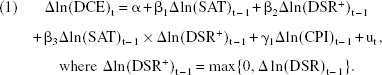
To test the significance of this relationship, we estimated the following asymmetric growth model (see, e.g., Lamey et al. 2007):

\begin{matrix} Δ \ln {(D C E)}_{t} = α + β_{1} Δ \ln {(S A T)}_{t - 1} + β_{2} Δ \ln {(D S R^{+})}_{t - 1} \\ + β_{3} Δ \ln {(S A T)}_{t - 1} \times Δ l n {(D S R^{+})}_{t - 1} + γ_{1} Δ \ln {(C P I)}_{t - 1} + u_{t}, \\ where Δ \ln {(D S R^{+})}_{t - 1} = \max {0, Δ l n {(D S R)}_{t - 1}} . \end{matrix}

(1)

We take lagged values of all explanatory variables for the following reasons: (1) It is consistent with the hypothesis that changes in customer satisfaction explain future changes in spending; (2) a contemporaneous relationship would not contradict the traditional life-cycle or permanent-income models of consumption (Carroll, Fuhrer, and Wilcox 1994); (3) lagging the variables is also in line with prior studies that try to find predictors of household expenditure growth (e.g., Bram and Ludvigson 1998; Hall 1978; Murphy 2000), which facilitates comparisons with prior studies using other macroeconomic variables; and (4) when the explanatory variables are lagged, simultaneity problems are avoided. We tested whether there is evidence of serial correlation in the error term, in which case the error terms would not be orthogonal to the variables dated t – 1 (Carroll, Fuhrer, and Wilcox 1994). This was not the case. We also tested for the need to include the lagged dependent variable as an additional control variable, but this variable was not significant (p = .30).

We present empirical results in the second column of Table 2. Following Long and Ervin's (2000) recommendation, we use heteroskedasticity-consistent standard errors using HC3 to assess significance levels. The Bera-Jarque test did not indicate violations of the residuals’ normality assumption (p = .30), and Chow's forecast test assessed at every possible break point since the Q1:2003 indicated parameter stability. All variance inflation factors (maximum value = 1.36) were well below the rule-of-thumb value of 5.0 that Judge and colleagues (1988) advocate; accordingly, there was no evidence of problematic multicollinearity.

Table 2

PARAMETER ESTIMATES OF THE ASYMMETRIC GROWTH MODEL

	Base Model	Credit	Income	ICS
Intercept	.02^** (.00)	.01^** (.00)	.02^** (.00)	.02^** (.00)
Δln(SAT)_{t – 1}	.35^* (.03)	.41^** (.01)	.35^* (.03)	.34^* (.03)
Δln(DSR⁺)_{t – 1}	–.29^* (.02)	–.40^** (.01)	–.27 (.14)	–.26^* (.03)
Δln(SAT)_{t – 1} × Δln(DSR⁺)_{t – 1}	40.50^** (.01)	–42.14^* (.03)	–41.41^** (.01)	–38.69^* (.01)
ΔlnCPL_{t – 1}	–.60^* (.03)	–.66^* (.03)	–.62^* (.02)	–.55 (.08)
Δln(Credit)_{t – 1}		.22 (.07)
Δln(Income)_{t – 1}			.05 (.84)
Δln(ICS)_{t – 1}				.02 (.53)
R²	.30	.35	.31	.32
Adjusted R²	.23	.27	.22	.23

p < .05 (two-sided).

p < .01 (two-sided).

Notes: The dependent variable in all models is Δln(DCE). Δln(DSR⁺)_{– 1} = max{0, Δ ln(DSR)_{t – 1}}. Significance levels are determined on the basis of heteroskedasticity-consistent standard errors using HC3. Values in parentheses are two-sided p-values.

The asymmetric model in Equation 1 explains almost 25% of the variation in discretionary spending growth (R² = .30; adjusted R² = .23). Furthermore, β₁ is significant (β₁ = .35, p < .05), as is β₃ (–40.50, p < .01), in support of our previous propositions. We tested whether a drop in the debt ratio had an effect, but it did not, neither as main effect (p = .63) nor in interaction with the lagged change in satisfaction (p = .82). This supports Messinis, Henry, and Olekalns (2002, p. 667, italics added), who argue that there is habit modification “only when household indebtedness increases.” Therefore, satisfaction with the previous purchases influences future spending growth, regardless of the size of the drop in the debt ratio. In contrast, the net effect weakens when the DSR becomes larger, as indicated by the negative interaction with Δln(DSR⁺). The net impact remains positive and significant (5%) as long as the quarterly growth in the debt ratio does not exceed a certain threshold, corresponding to .14% (i.e., Δln[DSR⁺] < .0014) in our base model. We derived standard errors for the net effect using the delta rule (for marketing applications, see, e.g., Dekimpe and Hanssens 1995; Kelley 1947; Srinivasan et al. 2004). In our sample, Δln(DSR⁺) varied between 0 and .031 (3.1%).

In the 16 quarters of available data, the DSR either decreased (14 times) or increased (2 times) at a rate lower than this threshold. In those cases, past changes in customer satisfaction had a significant impact on subsequent spending growth. At the somewhat less stringent 10% level, the threshold becomes .27%, and the number of times when past changes in customer satisfaction had an impact increases to 20.

Robustness Checks

To validate our findings, we conducted three sets of robustness checks. First, the fit of our model, with an adjusted R-square of .23 was considerably higher than in prior studies. To assess whether the improved fit was due to idiosyncracies of the particular period (when all variables would do better), we implemented several test equations used in prior work (see, e.g., Carroll, Fuhrer, and Wilcox 1994; Ludvigson 2004; Murphy 2000) and regressed the change in consumer spending on lagged differences of, respectively, the income, credit, DSR, and consumer sentiment variables. The number of lags varied between 1 and 4. We used lagged differences (rather than lagged levels as in some prior studies) on the basis of prior unit root tests. The adjusted R-square of these models never exceeded .12.

Second, we checked whether our results were robust when adding other potential drivers of spending growth, such as lagged changes in consumer sentiment (as in Bram and Ludvigston 1998), income (suggested in Hall 1978), and credit (studied in Ludvigson 1999). The corresponding estimates appear in the final columns of Table 2. In all instances, β₁ (for the main effect of satisfaction changes) and β₃ (for the interaction effect with the debt service variable) remained significant and of comparable magnitude to the base model. Thus, the parameter estimates were robust across alternative specifications and suggest that customer satisfaction has predictive power above and beyond information contained in those other variables.

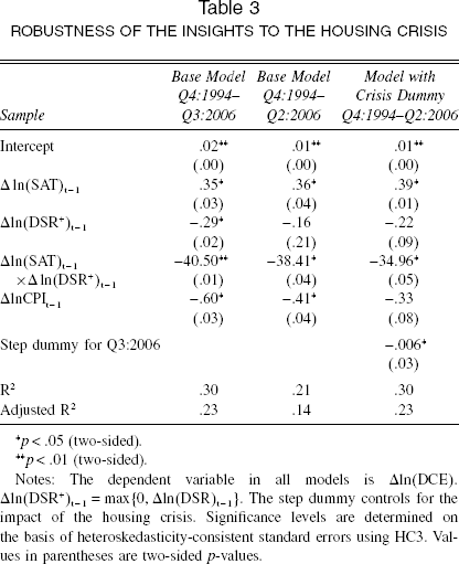
In further testing, we added eight observations to the sample, Q3:2006–Q2:2008. These observations reflect changes in consumer expenditures during the recent financial/housing crisis (BBC News 2007), a crisis so severe that it has been compared with the Great Depression (e.g., USA Today; see Pickler 2008). The question here is, Do our results hold in a period of great economic turmoil? As Table 3 (Column 3) shows, our key findings remain (both the main and the interaction effect) significant, with parameter estimates of comparable magnitude to what we had before (for β₁, .35 versus .36; for β₃, −40.50 versus 38.41). However, the overall fit of the model dropped considerably, as the adjusted R-square dropped 40.1%, from .23 to .14.

Table 3

Robustness of the Insights to the Housing Crisis

Sample	Base Model Q4:1994–Q3:2006	Base Model Q4:1994–Q2:2006	Model with Crisis Dummy Q4:1994–Q2:2006
Intercept	.02^** (.00)	.01^** (.00)	.01^** (.00)
Δ ln(CSAT)_{t – 1}	.35^* (.03)	.36^* (.04)	.39^* (.01)
Δln(DSR⁺)_{t – 1}	-.29^* (.02)	–.16 (.21)	-.22 (.09)
Δln(SAT)_{t – 1} × Δ ln(DSR⁺)_{t – 1}	–40.50^** (.01)	–38.41^* (.04)	–34.96^* (.05)
ΔlnCPI_{t – 1}	-.60^* (.03)	–.41^* (.04)	–.33 (.08)
Step dummy for Q3:2006			–.006^* (.03)
R²	.30	.21	.30
Adjusted R²	.23	.14	.23

p < .05 (two-sided).

p <. 01 (two-sided).

Notes: The dependent variable in all models is Δln(DCE). Δln(DSR+)_{t – 1} = max{0, Δln(DSR)_{t – 1}}. The step dummy controls for the impact of the housing crisis. Significance levels are determined on the basis of heteroskedasticity-consistent standard errors using HC3. Values in parentheses are two-sided p-values.

Adding a step dummy to allow for a structural change in the drift term (in the same spirit as Perron [1989], who controlled for the impact of the depression following the stock market crash of 1929 in his models of U.S. GDP), restored the fit of the model (adjusted R² = .23), again with similar parameter estimates for the satisfaction-related variables (see Column 4 of Table 3). Although the model clearly exhibits an intercept shift, and therefore reflects a different regime for consumer spending growth, the parameters for the satisfaction-related variables remained similar. Formal tests for a structural break in the slope parameters did not suggest significance, neither for the main effect (p = .43) nor for the interaction effect (p = .52). Thus, although the recent financial/housing crisis played havoc with consumer spending, the underlying relationships are robust and remain intact.

Conclusion

We argue that a major marketing variable may have been overlooked in the debate on whether consumer spending growth can be predicted. We find that customer satisfaction explains a good deal of future growth in discretionary spending, both as a main effect and in combination with household DSR. We show that the explanatory power of these variables is considerably higher than of other variables, such as credit, income, and consumer sentiment, which have all been examined in prior research. In addition, our findings contribute to the growing evidence that consumers react differently to positive versus negative changes in their financial situation. In line with Messinis, Henry, and Olekalns (2002), we find that past consumption experience weakens as debt increases. When debt is reduced, the main effect remains.

As we indicated previously, reports on expected changes in consumer spending may lead marketing managers to alter their marketing plans. By then, however, it may be too late. Marketing managers should not react only to the evolution in consumer spending. Our results suggest that good marketing, which leaves customers satisfied, also helps proactively curb spending reductions. Although this has already been suggested at the firm (Boulding et al. 1993) and industry (Fornell et al. 1996) levels, our results show that this is more than a zero-sum game in which customer-oriented firms (industries) gain at the expense of competition. Rather, when the overall quality of offerings improves and customer satisfaction increases, the aggregate level of consumer spending increases as well, unless the household debt service creates too much of a budget constraint. As such, while offering easy credit (or even zero financing) may allow firms to temporarily protect sales, the resultant increase in customer debt not only poses a threat to the long-term health of the economy but also undermines the potential contribution of good (i.e., satisfaction-enhancing) marketing. Pauwels and colleagues (2004) make a similar observation: Although innovations increased the long-term financial valuation of car manufacturers, promotional incentives (e.g., 0% financing) had a negative impact on company capitalization, despite the sales increase.

From a theoretical point of view, our findings contribute to a growing body of empirical literature that provides evidence against the permanent-income hypothesis and the related life-cycle hypothesis in aggregate data and suggest that there is another fundamental factor at play in explaining why consumers spend—namely, a search for gratification or the satisfaction derived from consumption. From a practical point of view, economic forecasters might benefit from paying closer attention to marketing-related variables when predicting consumer spending growth.

Our study has several limitations that suggest areas for future inquiry. Our findings are confined to the United States, and it would be prudent to generalize them to other countries. Consumers are not the same in all countries. They differ in propensity to save, risk attitude, long-term orientation, and so forth, and it is not clear how consumption utility and debt service interact with respect to spending growth. Similarly, we examined discretionary expenditures. It might be useful to consider other potential marketing drivers of nondiscretionary spending.

In addition to the obvious relevance for the economy in general, the implications for marketing are considerable. A better understanding of consumer spending growth should result in better marketing plans and better sales forecasts, which in turn should lead to superior decisions in all major areas of marketing, including products, pricing, promotion, distribution, capacity planning, and staffing decisions. In addition, recent research has emphasized the value of many marketing metrics to stock market analysts (e.g., Lehmann 2004; Rust et al. 2004). The findings of this study suggest that macroeconomists might also benefit from a closer monitoring of marketing metrics.

References

Anderson

Eugene, W.

, (1998), “Customer Satisfaction and Word-of-Mouth,” Journal of Service Research, 1(1), 1–14.

Anderson

Eugene W.

, Fornell

Claes

, and Lehmann

Donald R.

, (1994), “Customer Satisfaction, Market Share and Profitability: Findings from Sweden,” Journal of Marketing, 58(July), 53–66.

Anderson

Eugene W.

, Fornell

Claes

, and Mazvancheryl

Sanal

, (2004), “Customer Satisfaction and Shareholder Value,” Journal of Marketing, 68(October), 172–85.

Anderson

Eugene W.

, Fornell

Claes

, and Rust

Roland T.

, (1996), “Customer Satisfaction, Productivity and Profitability: Differences Between Goods and Services,” Marketing Science, 16(2), 129–45.

BBC News (2007), “The Downturn in Facts and Figures,” (November 21), (accessed November 5, 2009), [available at http://news.bbc.co.uk/2/hi/business/7073131.stm].

Boulding

William

, Kalra

Ajay

, Staelin

Richard

, and Zeithaml

Valarie A.

, (1993), “A Dynamic Process Model of Service Quality: From Expectations to Behavioral Intentions,” Journal of Marketing Research, 30(February), 7–27.

Bram

Jason

, and Ludvigson

Sydney

, (1998), “Does Consumer Confidence Forecast Household Expenditure? A Sentiment Index Horse Race,” Economic Policy Review: Federal Reserve Bank of New York, 4(June), 59–78.

Bureau of Economic Analysis (2008), National Income and Product Accounts, U.S. Department of Commerce, (accessed August 28, 2008), [available at http://bea.gov/national/nipaweb/Select-Table.asp?Selected=N].

Bureau of Labor Statistics (2008), “Consumer Price Index Archived News Releases,” (accessed August 28, 2008), [available at http://www.bls.gov/CPI/].

10.

Carroll

Christopher D.

, Fuhrer

Jeffrey C.

, and Wilcox

David W.

, (1994), “Does Consumer Sentiment Forecast Household Spending? If So, Why?” American Economic Review, 84(December), 1397–1408.

11.

Carruth

Alan

, and Dickerson

Andrew

, (2003), “An Asymmetric Error Correction Model of UK Consumer Spending,” Applied Economics, 35(6), 619–30.

12.

Case

Karl E.

, Quigley

John M.

, and Shiller

Robert J.

, (2001), “Comparing Wealth Effects: The Stock Market Versus the Housing Market,” NBER Working Paper No. 8606, (November).

13.

Chicago Tribune (2008), “Fed Rate Cut Announced Today,” (October 29), (accessed September 21, 2009), [available at http://www.chicagotribune.com/business/chi-fed-rate-cut-approved-081028-ht,0,1630477.story].

14.

Cornell

Bradford

, (1977), “Spot Rates, Forward Rates, and Exchange Market Efficiency,” Journal of Financial Economics, 5(August), 56–65.

15.

Danaher

Peter J.

, and Rust

Roland T.

, (1996), “Indirect Financial Benefits from Service Quality,” Quality Management Journal, 3(2), 63–75.

16.

Dekimpe

Marnik G.

, and Hanssens

Dominique M.

, (1995), “The Persistence of Marketing Effects on Sales,” Marketing Science, 14(Winter), 1–21.

17.

Deleersnyder

Barbara

, Dekimpe

Marnik G.

, Sarvary

Miklos

, and Parker

Philip M.

, (2004), “Weathering Tight Economic Times: The Sales Evolution of Consumer Durables over the Business Cycle,” Quantitative Marketing and Economics, 2(4), 347–83.

18.

Deleersnyder

Barbara

, Geyskens

Inge

, Gielens

Katrijn

, and Dekimpe

Marnik G.

, (2002), “How Cannibalistic Is the Internet Channel? A Study on the Newspaper Industry in the United Kingdom and the Netherlands,” International Journal of Research in Marketing, 19(4), 337–48.

19.

Fama

Eugene, F.

, (1970), “Efficient Capital Markets: A Review of Theory and Empirical Work,” Journal of Finance, 25(2), 383–417.

20.

Federal Reserve Board (2008), “Federal Reserve Statistical Release: Consumer Credit,” Federal Reserve Board release, (accessed August 28, 2008), [available at http://www.federal-reserve.gov/releases/g19/].

21.

Fornell

Claes

, Johnson

Michael D.

, Anderson

Eugene W.

, Cha

Jaesung

, and Everitt-Bryant

Barbara

, (1996), “The American Customer Satisfaction Index: Nature, Purpose, and Findings,” Journal of Marketing, 60(October), 7–18.

22.

Fornell

Claes

, Mithas

Sunil

, Morgeson

Forrest

, and Krishnan

M.S.

, (2006), “Customer Satisfaction and Stock Prices: High Returns, Low Risk,” Journal of Marketing, 70(January), 3–14.

23.

Franses

Philip Hans

, and Koop

Gary

, (1998), “On the Sensitivity of Unit-Root Inference to Nonlinear Data Transformations,” Economics Letters, 59(1), 7–15.

24.

Friedman

Milton, A.

, (1957), A Theory of the Consumption Function. Princeton, NJ: Princeton University Press.

25.

Grande

Carlos

, (2006), “Businesses Keep Tight Grip on Advertising amid Economy Fears,” Financial Times, (July 17), (accessed September 21, 2009), [available at http://www.ft.com/cms/s/0/4934a614-1530-11db-b391-0000779e2340.html?nclick_check=1].

26.

Gray

Tim

, (2004), “Sunday Money: Investing: The Bounce Is Back for Sneaker Makers,” The New York Times, (May 23), (accessed September 21, 2009), [available at http://www.nytimes.com/2004/05/23/business/sunday-money-investing-the-bounce-is-back-for-sneaker-makers.html].

27.

Gruca

Thomas S.

, and Rego

Lopo L.

, (2005), “Customer Satisfaction, Cash Flow, and Shareholder Value,” Journal of Marketing, 69(July), 115–30.

28.

Guerrera

Francesco

, Weitzman

Hal

, and Kim

Victoria

, (2007), “‘Economic Pressures’ Hit Wal-Mart Profit,” Financial Times, (August 14), (accessed September 21, 2009), [available at http://www.ft.com/cms/s/0/7b960e46-4aa3-11dc-95b5-0000779fd2ac.html].

29.

Gupta

Sunil

, and Zeithaml

Valarie

, (2006), “Customer Metrics and Their Impact on Financial Performance,” Marketing Science, 25(November–December), 718–39.

30.

Hall

Robert, E.

, (1978), “Stochastic Implications of the Life-Cycle/Permanent Income Hypothesis: Theory and Evidence,” Journal of Political Economy, 86(6), 971–87.

31.

Homburg

Christian

, Koschate

Nicole

, and Hoyer

Wayne D.

, (2005), “Do Satisfied Customers Really Pay More? A Study of the Relationship Between Customer Satisfaction and Willingness to Pay,” Journal of Marketing, 69(April), 84–96.

32.

Johnson

Kathleen W.

, and Li

Geng

, (2007), “Do High Debt Payments Hinder Household Consumption Smoothing?”Finance and Economics Discussion Series 2007–52, Federal Reserve Board, Washington, DC.

33.

Johnson

Michael D.

, Anderson

Eugene W.

, and Fornell

Claes

, (1995), “Rational and Adaptive Performance Expectations in a Customer Satisfaction Framework,” Journal of Consumer Research, 21(March), 695–707.

34.

Judge

George G.

, Carter Hill

, Griffiths

William E.

, Lütkepohl

Helmut

, and Lee

Tsoung-Chao

, (1988), Introduction to the Theory and Practice of Econometrics. New York: John Wiley & Sons.

35.

Katona

George

, (1975), Psychological Economics. New York: Elsevier Scientific Publishing.

36.

Katona

George

, (1979), “Toward a Macropsychology,” American Psychologist, 34(February), 118–26.

37.

Keiningham

Timothy L.

, Cooil

Bruce

, Aksoy

Lerzan

, Andreassen

Tor W.

, and Weiner

Jay

, (2007), “The Value of Different Customer Satisfaction and Loyalty Metrics in Predicting Customer Retention, Recommendation, and Share-of-Wallet,” Managing Service Quality, 17(4), 361–84.

38.

Keiningham

Timothy L.

, Perkins-Munn

Tiffany

, and Evans

Heather

, (2003), “The Impact of Customer Satisfaction on Share-of-Wallet in a Business-to-Business Environment,” Journal of Service Research, 6(1), 37–50.

39.

Kelley

T.L.

, (1947), Fundamentals of Statistics. Cambridge, MA: Harvard University Press.

40.

Lahart

Justin

, (2003), “Spending Our Way to Disaster,” CNNMoney.com, (October 3), (accessed September 21, 2009), [available at http://money.cnn.com/2003/10/02/markets/consumerbubble/].

41.

Lamey

Lien

, Deleersnyder

Barbara

, Dekimpe

Marnik G.

, and Steenkamp

Jan-Benedict E.M.

, (2007), “How Business Cycles Contribute to Private-Label Success: Evidence from the United States and Europe,” Journal of Marketing, 71(January), 1–15.

42.

Lehmann

Donald, R.

, (2004), “Metrics for Making Marketing Matter,” Journal of Marketing, 68(October), 73–75.

43.

Shibo

, Sun

Baohong

, and Wilcox

Ronald T.

, (2005), “Cross-Selling Sequentially Ordered Products: An Application to Consumer Banking Services,” Journal of Marketing Research, 42(May), 233–39.

44.

Long

J. Scott

, and Ervin

Laurie H.

, (2000), “Using Heteroscedasticity Consistent Standard Errors in the Linear Regression Model,” American Statistician, 54(3), 217–24.

45.

Ludvigson

Sydney, C.

, (1999), “Consumption and Credit: A Model of Time-Varying Liquidity Constraints,” Review of Economics and Statistics, 81(3), 434–47.

46.

Ludvigson

Sydney, C.

, (2004), “Consumer Confidence and Consumer Spending,” Journal of Economic Perspectives, 18(2), 29–50.

47.

Messinis

George

, Henry

Ólan

, and Olekalns

Nills

, (2002), “Rational Habit Modification in Consumption,” Economic Modeling, 19(4), 665–78.

48.

Mittal

Vikas

, Anderson

Eugene W.

, Sayrak

Akin

, and Tadikamalla

Pandu

, (2005), “Dual Emphasis and the Long-Term Financial Impact of Customer Satisfaction,” Marketing Science, 24(4), 544–58.

49.

Modigliani

Franco

, (1971), “Monetary Policy and Consumption,” in Consumer Spending and Monetary Policy: The Linkages, Conference Series No. 5. Boston: Federal Reserve Bank of Boston, 9–84.

50.

Murphy

Robert, G.

, (1998), “Household Debt and Consumer Spending,” Business Economics, (July 1), (accessed September 21, 2009), [available at http://findarticles.com/p/articles/mi_m1094/is_n3_v33/ai_20946410/].

51.

Murphy

Robert, G.

, (2000), “Does Household Debt Forecast Consumer Spending?” working paper, Department of Economics, Boston College.

52.

Nijs

Vincent

, Dekimpe

Marnik G.

, Steenkamp

Jan-Benedict E.M.

, and Hanssens

Dominique M.

, (2001), “The Category Demand Effects of Price Promotions,” Marketing Science, 20(1), 1–22.

53.

Oliver

Richard, L.

, (1997), Satisfaction: A Behavioral Perspective on the Consumer. Boston: Richard D. Irwin/McGraw-Hill.

54.

Pauwels

Koen

, Silva-Risso

Jorge

, Srinivasan

Shuba

, and Hanssens

Dominique M.

, (2004), “New Products, Sales Promotions, and Firm Value: The Case of the Automobile Industry,” Journal of Marketing, 68(October), 142–56.

55.

Perron

Pierre

, (1989), “The Great Crash, the Oil Price Shock, and the Unit Root Hypothesis,” Econometrica, 57(November), 1361–1401.

56.

Nedra

Pickler

, (Associated Press) (2008), “Obama Makes a Final Pitch in Radio Address,” USA Today, (November 1), (accessed September 21, 2009), [available at http://www.usatoday.com/news/politics/2008-11-01-108765316_x.htm].

57.

Rao

Ramesh K.S.

, and Bharadwaj

Neeraj

, (2008), “Marketing Initiatives, Expected Cash Flows, and Shareholders’ Wealth,” Journal of Marketing, 72(January), 16–26.

58.

Rust

Roland T.

, Ambler

Tim

, Carpenter

Gregory S.

, Kumar

, and Srivastava

Rajendra K.

, (2004), “Measuring Marketing Productivity: Current Knowledge and Future Directions,” Journal of Marketing, 68(October), 76–89.

59.

Rust

Roland T.

, and Zahorik

Anthony J.

, (1993), “Customer Satisfaction, Customer Retention, and Market Share,” Journal of Retailing, 69(Summer), 193–215.

60.

Shea

John

, (1995), “Myopia, Liquidity Constraints, and Aggregate Consumption: A Simple Test,” Journal of Money, Credit and Banking, 27(3), 798–805.

61.

Srinivasan

Shuba

, Pauwels

Koen

, Hanssens

Dominique M.

, and Dekimpe

Marnik G.

, (2004), “Do Promotions Benefit Manufacturers, Retailers, or Both?” Management Science, 50(5), 617–29.

62.

University of Michigan (2008), Surveys of Consumers, University of Michigan Survey Research Center, (accessed August 28, 2008), [available at http://www.sca.isr.umich.edu/data-archive/mine.php].

63.

Zeithaml

Valarie A.

, Bolton

Ruth N.

, Deighton

John

, Keiningham

Timothy L.

, Lemon

Katherine N.

, and Andrew Peterson

, (2006), “Forward-Looking Focus: Can Firms Have Adaptive Foresight?” Journal of Service Research, 9(2), 168–83.