Identifying the Presence and Cause of Fashion Cycles in Data

Abstract

Fashions and conspicuous consumption play an important role in marketing. In this article, the author presents a three-pronged framework to analyze fashion cycles in data composed of (1) algorithmic methods for identifying cycles, (2) a statistical framework for identifying cycles, and (3) methods for examining the drivers of such cycles. In the first module, the author identifies cycles by pattern-matching the amplitude and length of cycles observed to a user-specified definition. In the second module, the author defines the conditional monotonicity property, derives conditions under which a data-generating process satisfies it, and demonstrates its role in generating cycles. A key challenge in estimating this model is the presence of endogenous lagged dependent variables, which the author addresses using system generalized method of moments estimators. Third, the author presents methods that exploit the longitudinal and geographic variations in agents' economic and cultural capital to examine the different theories of fashion. The author applies her framework to data on given names for infants, shows the presence of large-amplitude cycles both algorithmically and statistically, and confirms that the adoption patterns are consistent with Bourdieu's theory of fashion as a signal of cultural capital.

Keywords

fashion name choices

Fashion

Fashion, as a phenomenon, has existed and flourished since ancient times across a wide variety of conspicuously consumed products. The impact of fashion can be observed in all aspects of society and culture, including clothing, painting, sculpture, music, drama, dancing, architecture, and art (English 2007; Lipovetsky, Porter, and Sennett 1994). According to the prominent sociologist Blumer (1969), fashion appears even in redoubtable fields such as sciences, medicine, business management, and mortuary practices.

Fashion plays an important role in the marketing of many commercial products. For example, the U.S. apparel and footwear industry follows a seasonal fashion cycle, in the form of spring/summer and fall/winter collections. According to industry experts, a large chunk of the $300 billion that Americans spend on apparel/footwear annually is fashion driven rather than need driven. Fashion also influences the success of other conspicuously consumed products such as electronic gadgets, furniture, and cars (Liu and Donath 2006; Seymour 2008). For instance, the 1950s saw the rise and fall of the tailfin craze in car designs. Even though tailfins were completely nonutilitarian, they contributed to the phenomenal success of Cadillacs and other cars sporting fins (Gammage and Jones 1974).

Given the widespread impact of fashion and its economic importance, it is essential that marketers develop frameworks to reliably identify fashion cycles in data and examine their drivers. However, to date there is no empirical framework to study fashion cycles. Furthermore, no research has examined whether the cycles observed in data are consistent with any of the proposed theories of fashion. Indeed, apart from a few early descriptive works by Richardson and Kroeber (1940) and Robinson (1975), there is hardly any empirical work on fashion. In this article, I attempt to bridge this gap in the literature.

Framework for Analyzing Fashion Cycles

In the current research, I present a three-pronged framework to analyze fashions composed of (1) algorithms for identifying cycles, (2) statistical models for identifying cycles, and (3) methods for examining the drivers of fashion cycles. The first module consists of an algorithmic framework for identifying fashion cycles by pattern-matching the amplitude and length of cycles observed in the data to a user-specified definition of a cycle as satisfying certain minimum requirements on those dimensions. I also use algorithmic methods to characterize and identify recurring cycles, whereby each cycle is separated by a dormancy period that is allowed to be a function of the amplitude of the cycle. Taken together, these techniques enable me to characterize different types of cyclical patterns in data.

Although algorithmic identification of cycles is sufficient for many purposes, it suffers from user subjectivity. Thus, in the second module, I develop a statistical method to identify the presence of cycles. I define the conditional monotonicity property and derive the conditions under which a data-generating process satisfies this property. Specifically, an autoregressive process of order p (AR(p)) is conditionally monotonic if it is nonstationary and continues to increase (decrease) in expectation if it was on an increasing (decreasing) trend in the last (p – 1) periods. I then demonstrate that conditional monotonicity is necessary and sufficient to give rise to cycles.

A key challenge in estimating this model and establishing conditional monotonicity is the presence of potentially endogenous lagged dependent variables. In such cases, the two commonly used estimators—the random-effects estimator and fixed-effects estimator—cannot be used (Nickell 1981). Although theoretically, I can solve this by finding external instruments for the endogenous variables, it is difficult to find variables that affect the lagged popularity of a fashion product but not its current popularity. I address this issue using system generalized method of moments (GMM) estimators that exploit the lags and lagged differences of explanatory variables as instruments (Blundell and Bond 1998; Shriver 2015).

Finally, in the third module, I expand my framework to examine the drivers of fashion. Although various drivers of fashion have been proposed, two signaling theories have gained prominence because of their ability to provide internally consistent reasoning for the rise and fall of fashions: wealth signaling theory (Veblen 1899) and cultural capital signaling theory (Bourdieu 1984). While existing analytical models of fashion assume one of these social signaling theories and examine the role of firms in fashion markets, they do not test the empirical validity of either of these theories (Amaldoss and Jain 2005; Pesendorfer 1995; Yoganarasimhan 2012a). In contrast, I present empirical tests to infer whether the patterns observed in data are consistent with one of these theories. I use aggregate data on the metrics of wealth and cultural capital of parents in conjunction with state-level name popularity data and exploit the geographical and longitudinal variation in these two metrics to correlate name adoption to the predictions of the two theories.

Name Choice Context

I apply my framework to the choice of given names (i.e., names given to newborn infants). I chose this as my context for four reasons. First, the choice of a child's name is an important conspicuous decision that parents make; therefore, it is a good area in which to examine fashion and conspicuous choices. Second, to establish the existence of cycles in a product category, I need data on a large panel of products for a significantly long period. My context satisfies this data requirement: the Social Security Administration (SSA) is an excellent source of data on given names at both the national and state levels, beginning in 1880. Third, it is a setting in which large cycles of popularity are observed, which makes it ideal for this study. Figure 1 depicts the rise and fall of the most popular male and female baby names from 1980. Note that at their peaks, these names were given to more than 80,000 babies on a yearly basis, which hints at the presence of cycles of large amplitude in this data. Fourth, to examine the impact of social drivers of fashion cycles, I need both time and geographic variation in agents' status in the society, which is available in the form of metrics on economic and cultural capital through U.S. Census data. Together, these factors make the context of given names ideal for studying fashion cycles.

Figure 1

POPULARITY CURVES OF THE TOP FEMALE AND MALE BABY NAMES FROM 1980

Findings

Using this framework, I provide a series of substantive results. First, I establish the existence of large-magnitude cycles in the names data using algorithmic methods. Of the names that have appeared in the top 50 in at least one year since 1940, more than 80% have experienced at least one cycle of popularity, and a significant fraction (approximately 30%) of these has gone through two or more cycles. In data sets that include less popular names, the fraction of names with cycles is lower but still significant. For instance, of all female names that have been in the top 500 in at least one year since 1940, more than 75% have gone through at least one cycle of popularity. I also find that a significant fraction of names have gone through at least two cycles of popularity and find evidence for patterns shaped like and .

Second, I apply my statistical framework to the name choice data and show that it follows a second-order autoregressive (AR(2)) process that satisfies the conditional monotonicity property. I show that the names data exhibit nonstationarity (i.e., they have a unit root) and follow the direction of the movement from the last period, thereby satisfying the two conditions for conditional monotonicity. These results are robust across different types of data and model specifications. Thus, there is statistical evidence that the data-generating process satisfies properties that lead to cycles when sampled over significantly long periods of time.

Third, I exploit the longitudinal and geographical variations in cultural and economic capital to show that these cycles are consistent with Bourdieu's cultural capital signaling theory. I present three findings in this context. First, I show that states with higher average cultural capital are the first to adopt names that eventually become fashionable; they are then followed by the states with less cultural capital. Similarly, the states with higher average cultural capital are the first to abandon increasingly popular names. In other words, the rate of adoption is higher among the “cultured states” at the beginning of the cycle, whereas the opposite is true at the end of cycle. Second, I find that adoption among the cultured states has a positive impact on the adoption of the general population, while adoption among less cultured states has a negative impact on the overall adoption. Third, I do not find any such parallel results for economic capital. Taken together, these results provide support for Bourdieu's theory in the name choice context.

The results have implications for a broad range of fashion firms. First, my empirical framework enables firms to test for the presence of fashion cycles in their context. Second, it allows them to uncover the social signaling needs of their consumers, which in turn would help them target the right consumers at different stages of the fashion cycle. For example, if a firm finds that its products serve as signals of cultural capital, it can initially seed information with cultured consumers and then release information to the larger population in a controlled manner to maximize profits.

Related Literature

The current research relates to three broad streams of literature in marketing, sociology, finance, and economics. First, it relates to the theoretical literature on conspicuous consumption and fashion cycles. Karni and Schmeidler (1990) present one of the earliest models of fashion with two social groups, high and low. Agents in both groups value products used by “high types” but not those used by “low types.” In this setting, they show that fashion cycles can arise in equilibrium. Similarly, Corneo and Jeanne (1994) show that fashion cycles may arise out of information asymmetry. On a related front, Amaldoss and Jain (2005) study the pricing of conspicuous goods. Pesendorfer (1995) adopts the view that fashion is a signal of wealth (Veblen 1899), adds a firm to the mix, and goes on to show that a monopolist produces fashion in cycles to enable high types to signal their wealth. In contrast, Yoganarasimhan (2012a) presents a model in which agents want to signal that they are “in the know” or have access to information. In this setting, she shows that a fashion firm may want to strategically cloak information on its most fashionable products to allow for the signaling game between consumers.

Second, the current research relates to the macroeconomic literature on identification of business cycles from data pioneered by Burns and Mitchell (1946). Recent work has advocated the use of band-pass filters to separate cycles from short-term fluctuations and long-term trends under the assumption that cycles indeed exist and that cycle length falls under certain limits (Baxter and King 1999; Hodrick and Prescott 1997). These methods are designed to work with a small number of time series that exhibit similar behaviors. Furthermore, they do not offer any insights on the factors that give rise to cycles. My approach differs from these methods in three important ways: (1) I do not know whether a given name has gone through a cycle, and I do not limit the length of the cycles; (2) I have a very large number of names, and there is no co-movement or even similarity in the cycles across names; and (3) I am interested in exploring the underlying reasons for fashion cycles and thus need a methodology that can accommodate endogenous explanatory variables.

Third, the current research relates to the finance literature on identifying stock market bubbles using nonstationarity tests (Charemza and Deadman 1995; Diba and Grossman 1988; Evans 1991). The key difference between these articles and the current research is that they define a bubble as any long-term deviation from the stable mean of an autoregressive process. Thus, nonstationarity tests are sufficient to identify bubbles. In contrast, I am interested in fashion cycles, which are defined as long-term deviations characterized by consecutive increases followed by consecutive decreases (or vice versa) and are caused by social signaling. I show that nonstationarity is necessary but not sufficient to identify cycles, and I go on to define conditional monotonicity and demonstrate its ability to establish the presence of cycles. As with the previous methods, these cannot provide information about the drivers of fashion cycles.

This article also contributes to the literature on the measurement of social effects in marketing. For some recent developments in this area, see Chintagunta, Gopinath, Venkataraman (2010), Nair, Manchanda, and Bhatia (2010), Sun, Zhang, and Zhu (2014), Tellis, Niraj, and Yin (2009), Toubia, Goldenberg, and Garcia (2014), and Yoganarasimhan (2012b). Finally, this article relates to the literature on name choice, which I discuss in the next section.

The Naming Decision

How do parents choose names, and why does the popularity of a name change over time? These are interesting questions that have attracted the attention of researchers in various domains. Sociologists were among the first to study names, and early works in this area include Rossi (1965), Taylor (1974), Lieberson and Bell (1992), Lieberson and Lynn (2003), and Lieberson (2000). More recently, in a descriptive study, Hahn and Bentley (2003) show that naming patterns can be characterized using power-law distributions and random regenerative models. Similarly, Gureckis and Goldstone (2009) include the effect of past adoptions to build a predictive model of name choice. Berger and Le Mens (2009) show that the speed of a name's adoption is correlated with its speed of abandonment. Drawing on a survey of expecting parents, they argue that this phenomenon stems from negative perceptions of fads. Although these studies demonstrate some naming patterns and provide preliminary evidence on the sociological aspects of name choice, they do not empirically establish the presence of cycles in the data or examine drivers of these cycles—which is the focus of this article.

Next, I present a discussion of factors that potentially affect parents' naming decisions. Subsequently in the article, I discuss how the empirical model controls for these factors.

Name Attributes

The popularity of a name is likely to depend on its attributes. For example, short names are easy to speak and spell, which makes them attractive to many parents (e.g., John vs. Montgomery). Parents may also prefer names that symbolize positive imagery and qualities, such as bravery (Richard), charm (Grace), and beauty (Helen, Lily).

Familial and Religious Reasons

Traditionally, newborns were named after their relatives. For instance, first-born boys were named after their father or paternal grandfather and first-born girls after their paternal grandmother. However, Rossi (1965) finds that this custom has been on a decline due to the rise of nuclear families.

Religious beliefs can also influence name choice. Many long-term popular names such as Joseph and Daniel have Biblical origins. However, Lieberson (2000) finds no correlation between church attendance and popularity of Biblical names in the United States and the United Kingdom. Even though some Biblical names have remained popular (e.g., Samuel, Seth), their choice is likely driven by other considerations, because many others have declined in popularity (e.g., Michael, Paul).

Assimilation and Differentiation

Researchers have shown that names associated with an obvious ethnic or minority population can have a negative impact on a child's future employment and success (Bertrand and Mullainathan 2004). Recognizing this, minority parents may choose conventional names to avoid discrimination and integrate their children into mainstream society. Consistent with this theory, Mencken (1963) finds that names that were popular among Norwegian immigrants (e.g., Leif, Thorvald, Nils) suffered a rapid loss in popularity after their immigration to the United States.

In contrast, some minority parents may try to differentiate their children from the majority by choosing names that highlight their distinctive ethnic background. Fryer and Levitt (2004) find that African American parents chose increasingly distinctive names in the 1970s, often with African roots, to emphasize their “blackness.” Of course, neither of these effects are at play for non-black or non-ethnic names.

Celebrity Names

Popular entertainers, sports stars, and celebrities are often mentioned in the mass media, and this exposure can influence parents' name choices. However, prior research has refuted the idea that fashion cycles in names are caused by celebrities. First, many stars adopt names that are currently popular, which actually implies reverse causality. For example, “Marilyn” was already a popular name before Norma Jean Baker adopted it as her stage name (Marilyn Monroe), and the name actually declined in popularity in the following years. Second, not all celebrities' names become popular and not all names that become popular are those of celebrities. Third, in the few cases in which a name became popular around the same time as a rising celebrity, the resulting increase in its popularity has been minor compared with the magnitude of the usual cycles observed in the data. Finally, if celebrities cause popularity cycles in names, then, empirically, there should be no difference in the rate of adoption among different classes of people at different stages of the fashion cycle. For example, a celebrity theory cannot give rise to an adoption pattern in which wealthy or cultured parents are first to both adopt and abandon a name. For a detailed discussion of this idea, see Lieberson (2000).

Signaling Theories

Finally, parents may choose names to signal their (and their child's) high status in the society. Two kinds of signaling mechanisms can be at work.

Signal of wealth

Parents may choose certain names to signal their affluence. The wealth signaling theory would predict name cycles as follows: (1) wealthy parents first adopt certain names, which makes them signals of wealth; (2) less wealthy parents adopt these names in imitation of the wealthy, which dilutes their signaling values; (3) the wealthy abandon these names because they are no longer exclusive signals of wealth; and (4) when the wealthy abandon these names, their signaling value decreases even more, which leads to abandonment by the less wealthy. This entire process constitutes a fashion cycle.

There is some support for this theory in the literature. Some sociologists have argued that the use of middle names by the English middle class is an imitation of the British aristocratic practice (Withycombe 1977). Others have provided correlational evidence that suggests that names popular among the wealthy were later adopted by the less wealthy (Lieberson 2000; Taylor 1974). However, the evidence in these studies is suggestive rather than conclusive.

Signal of cultural capital

Parents may choose names to signal their cultural capital and artistic temperament, and such an incentive can also give rise to cycles in the popularity of names (following the same reasoning as that used in the context of wealth-based fashion cycles). Indeed, Kisbye (1981) provides some evidence for this theory. In his study of English names in nineteenth-century Aarhus (Denmark), he finds an increase in the use of English names in the earlier part of the century (corresponding with the introduction of English books by Shakespeare, Dickens, and others), followed by a decrease toward the end of the century. Kisbye argues that English names were first adopted by the cultured or well-read Danes. However, toward the end of the nineteenth century, the less cultured residents obtained access to these previously obscure texts and started adopting English names, which in turn diluted their signaling value and led to their eventual decline. Although Kisbye does not provide concrete evidence to substantiate this speculation, his study suggests that names can be used as a vehicle to signal cultural capital. Similarly, Lieberson and Bell (1992) and Levitt and Dubner (2005) also provide some correlational evidence for the cultural capital signaling theory.¹

Their evidence is purely correlational (i.e., they do not control for other factors that could simultaneously drive name choices). In a critical commentary on Lieberson and Bell (1992), Besnard (1995) counters that most of the names popular among the highly educated in the early parts of the cycles Lieberson and Bell studied were also popular among the larger population. In addition, he asserts that their findings are unlikely to be meaningful given their short time frame of 13 years. My own analysis suggests that name cycles are, on average, much longer than 13 years.

By definition, signaling theories require an action to be not only costly but also differentially costly across types for it to serve as a credible signal of the sender's type. Given that names are free, at the first glance neither of these signaling theories may be expected to work. However, this would be a naive inference because the cost of gathering information on the set of names popular among the high types (in wealth or culture) could vary with the parents' own wealth and cultural capital. There is considerable evidence on network homophily (McPherson, Smith-Lovin, and Cook 2001). Researchers have found that social networks are strongly homophilous on both wealth and cultural capital. For example, Marsden (1990) finds that approximately 30% of personal networks are highly homophilous on education, which is one of the strongest indicators of cultural capital (see the “Cultural Capital” subsection). This homophily has powerful implications for people's access to information. If cultured people live in similar neighborhoods, attend similar cultural events, work in similar environments, and interact more with each other than with those outside their group, it is easier for a cultured parent (vs. a less cultured parent) to obtain information on the names that other cultured people have given their children. Thus, network homophily can give rise to heterogeneity in signaling costs across classes of people, thereby enabling names to serve as signals of parents' types. In a subsequent section, I examine whether the name cycles are consistent with one of these two signaling theories, after controlling for the aforementioned alternative explanations.

Data

I use two types of data in this study: (1) data on popularity of names, and (2) data on the cultural and economic capital of parents. I elaborate on these in the following subsections.

Data on Names

The data on names come from the SSA, the most comprehensive source of given names in the United States. All newborn U.S. citizens are eligible for a Social Security Number (SSN), and their parent(s) can easily apply for one while registering the newborn's birth. Although getting an SSN for a child is optional, almost all parent(s) choose to do so because an SSN is necessary to declare the child as a dependent in tax returns, open a bank account in the child's name, and obtain health insurance for the child.² The SSA therefore has information on the number of children of each sex who were given a specific name, for each year, starting in 1880. The SSA was established in 1935 and became fully functional only in 1937. Many people born before 1937 never applied for an SSN, and the data from 1880 to 1937 constitute a partial sample of the names from that period. Therefore, I restrict my empirical analysis to the data from 1940 to 2009.

There is a small discrepancy between the number of annual registered births and number of SSNs assigned. This may be due to the fact that some infants die before the assignment of SSNs. Alternately, a small set of parents may choose not to participate in the process for personal reasons.

These data are available at both national and state levels. At the national level, for each name i, I have information on the number of babies given name i in time period t, which I denote as ni_t. Because the data of interest start from 1940, t = 1 denotes the year 1940. The name identifier i is sex-specific. For example, the name “Addison” is given to both male and female babies, but I assign different identifiers to the two Addisons. To preserve privacy, if a name has been given to fewer than five babies in a year, the SSA does not release this number for that particular year. In such cases, ni_t is treated as 0. The state-level data are available for all 50 U.S. states. nij_t denotes the number of babies given name i in state j in time period t. As in the national data set, n_ijt is also left-truncated at 5, in which case I treat it as 0.

For each name i, I construct the following variables:

•

s_i = the sex of name i (s_i = 1 if i is a female name, and s_i = 0 if it is a male name),

•

l_i = the number of characters in name i, and

•

bib_i = the number of times that name i appears in the Bible.

The SSA also furnishes data on the total number of SSNs issued to newborns each year both nationally and statewide. I use these data to construct the following variables:

•

Γ_{s_it} = total number of babies of sex s_i assigned SSNs in period t, nationally. Thus, Γ_0t and Γ_1t are the total number of male and female babies born in period t;

•

Γ_{s_ijt} = total number of babies of sex s_i assigned SSNs in state j in period t;

•

f_it = n_it/Γ_{s_it} is the fraction of babies of sex s_i given name i in period t; and

•

f_ijt = Γ_{s_ijt} is the fraction of babies of sex s_i given name i in period t within state j.

There are a total of 56,937 female and 33,745 male names in the data, but a small subset of these names account for a large portion of name choices. To focus the analysis on a representative sample of names, I work with the following four subsets of data:

•

Top50 data set: For each year starting with 1940, I collect the top 50 male and the top 50 female names given to newborns in the country. I then pool these names to form the Top50 data set.

•

Top100 data set: Same as the Top50 data set, but it includes names that have appeared in the top 100.

•

Top200 data set: Same as the Top50 data set, but it includes names that have appeared in the top 200.

•

Top500 data set: Same as the Top50 data set, but it includes names that have appeared in the top 500.

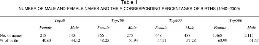
Table 1 shows the number of names in each data set by sex and also provides the fraction of total births that these data sets account for. For example, the Top500 data set contains a total of 1,468 female names, which together account for 60.99% of all female births from 1940 to 2009.

Table 1

NUMBER OF MALE AND FEMALE NAMES AND THEIR CORRESPONDING PERCENTAGES OF BIRTHS (1940–2009)

	Top50		Top100		Top200		Top500
	Female	Male	Female	Male	Female	Male	Female	Male
No. of names	218	143	366	275	648	488	1,468	1,115
% of births	40.63	44.12	48.25	51.94	54.71	57.28	60.99	61.67

Next, I examine the patterns in the name choice data. Table 2 shows the top ten female and male names for the years 1940, 1950, 1960, 1970, 1980, 1990, 2000, and 2009. It is clear that there is quite a bit of churn in popular names. For instance, of the ten most popular female names in 1990, only five remained in the top ten in 2000. To understand the patterns better, I plot the popularity of the top six female and males names from 1980 for the full span of the data (i.e., from 1880 to 2009; see Figures 2 and 3). The plots present clear visual evidence of cycles in the data.

Figure 2

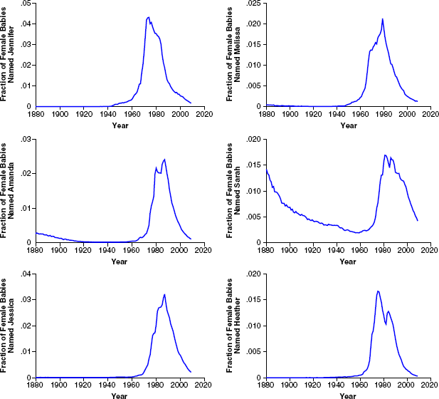
POPULARITY CURVES OF THE TOP SIX FEMALE BABY NAMES IN 1980

Figure 3

POPULARITY CURVES OF THE TOP SIX MALE BABY NAMES IN 1980

Table 2

TOP TEN FEMALE AND MALE NAMES IN 1940, 1950, 1960, 1970, 1980, 1990, 2000, AND 2009

	Rank
	1	2	3	4	5	6	7	8	9	10
1940
Female	Mary	Barbara	Patricia	Judith	Betty	Carol	Nancy	Linda	Shirley	Sandra
Male	James	Robert	John	William	Richard	Charles	David	Thomas	Donald	Ronald
1950
Female	Linda	Mary	Patricia	Barbara	Susan	Nancy	Deborah	Sandra	Carol	Kathleen
Male	James	Robert	John	Michael	David	William	Richard	Thomas	Charles	Gary
1960
Female	Mary	Susan	Linda	Karen	Donna	Lisa	Patricia	Deborah	Cynthia	Deborah
Male	David	Michael	James	John	Robert	Mark	William	Richard	Thomas	Steven
1970
Female	Jennifer	Lisa	Kimberly	Michelle	Amy	Angela	Melissa	Tammy	Mary	Tracy
Male	Michael	James	David	John	Robert	Christopher	William	Brian	Mark	Richard
1980
Female	Jennifer	Amanda	Jessica	Melissa	Sarah	Heather	Nicole	Amy	Elizabeth	Michelle
Male	Michael	Christopher	Jason	David	James	Matthew	Joshua	John	Robert	Joseph
1990
Female	Jessica	Ashley	Brittany	Amanda	Samantha	Sarah	Stephanie	Jennifer	Elizabeth	Lauren
Male	Michael	Christopher	Matthew	Joshua	Daniel	David	Andrew	James	Justin	Joseph
2000
Female	Emily	Hannah	Madison	Ashley	Sarah	Alexis	Samantha	Jessica	Elizabeth	Taylor
Male	Jacob	Michael	Matthew	Joshua	Christopher	Nicholas	Andrew	Joseph	Daniel	Tyler
2009
Female	Isabella	Emma	Olivia	Sophia	Ava	Emily	Madison	Abigail	Chloe	Mia
Male	Jacob	Ethan	Michael	Alexander	William	Joshua	Daniel	Jayden	Noah	Anthony

Data on Economic and Cultural Capital

To examine the two theories of fashion, I need data on the geographical (state-level) and longitudinal (yearly) variations in the economic and cultural capital of decision makers. I provide more information about these in the following subsections.

Economic capital

I use a state's median household income at period t as a measure of the economic capital of the decision makers from that state during t. The income data come from two sources: the decennial Census and the Social and Economic Supplements of the Current Population Survey (CPS). I retrieved data on the state-level median household income for 1970 and 1980 from the decennial census tables.³ For 1984–2009, I obtained annual state-level data on median household income from CPS. To calculate values for the intervening years in which income data are not directly available (1971–1979 and 1981–1983), I use linear interpolation, which is reasonable because a state's median income rarely exhibits wide year-to-year fluctuations.

Although the Census Bureau has asked income-related questions since 1940, the wording used in the question formulation in 1940, 1950, and 1960 is different from that in use now (family vs. household income), making it difficult to combine the data from the former years with the current data set.

The original data are in current dollars (i.e., reported dollars). To obtain a normalized measure of wealth, I need to correct for both inflation over time and geographic variations in cost of living. I do this using the revised 2009 version of the Berry-Fording-Hanson (2000; BFH) state cost of living index. This normalized metric is denoted as W_jt, the adjusted median household income of state j in period t. It is obtained as follows:

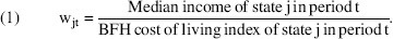
w_{jt} = \frac{Median income of state j in period t}{BFH cost of living index of state j in period t} .

(1)

The BFH index is a measure of how costly a state is compared with a median state in 2007 (the index for the two middle states, New Mexico and Wyoming, is set to 100 in 2007). Table 3 lists the top and bottom five wealthiest states based on w_jt for 1970, 1980, 1990, and 2000.

Table 3

TOP AND BOTTOM FIVE WEALTHIEST STATES^a AND TOP AND BOTTOM FIVE EDUCATED STATES^b

Year	Top Five Wealthy States		Bottom Five Wealthy States		Top Five Educated States		Bottom Five Educated States
Year	State	w_jt	State	w_jt	State	c_jt	State	c_jt
1970	Maryland	647.8	South Dakota	383.5	Colorado	4.2	Arkansas	–4.0
	Alaska	627	Maine	403.5	Alaska	3.4	West Virginia	–3.9
	California	621.6	Arkansas	408	Utah	3.3	Kentucky	–3.5
	Michigan	615.3	Vermont	408	Hawaii	3.3	Alabama	–2.9
	Texas	588.5	Mississippi	411.2	Maryland	3.2	Tennessee	–2.9
1980	Alaska	601.1	South Dakota	342.3	Colorado	6.7	West Virginia	–5.8
	Maryland	565	Maine	351	Alaska	4.9	Arkansas	–5.4
	Michigan	510.7	Vermont	364.1	Connecticut	4.5	Kentucky	–5.1
	Virginia	507.5	Mississippi	369.4	Maryland	4.2	Alabama	–4.0
	Texas	498.9	Arkansas	371	Hawaii	4.2	Mississippi	–3.9
1990	Alaska	672	South Dakota	383.8	Massachusetts	6.9	West Virginia	–8.0
	Maryland	646.3	North Dakota	389.4	Connecticut	6.9	Arkansas	–7.0
	Virginia	580.5	Mississippi	393.6	Colorado	6.7	Kentucky	–6.7
	Delaware	572.7	West Virginia	393.7	Maryland	6.2	Mississippi	–5.6
	New Jersey	551.9	Arkansas	407.3	New Jersey	4.6	Nevada	–5.0
2000	Maryland	677.6	West Virginia	407.3	Massachusetts	8.8	West Virginia	–9.6
	Alaska	645.3	Kentucky	413.5	Colorado	8.3	Arkansas	–7.7
	Minnesota	636.4	Louisiana	422.2	Maryland	7.1	Mississippi	–7.5
	Delaware	626.6	Maine	423.5	Connecticut	7.0	Kentucky	–7.3
	Virginia	607	Montana	432.1	New Jersey	5.4	Nevada	–6.2

Based on adjusted median household income.

Based on percentage of adults with a bachelor's degree.

Cultural capital

Cultural capital is defined as a person's knowledge of arts, literature, and culture (Bourdieu 1984; Dimaggio and Useem 1974). The most commonly used measure of cultural capital is education attainment, especially higher education (Cookson and Persell 1987; Lamont and Lareau 1988; Robinson and Gamier 1985).

I use the percentage of adults in state j with a bachelor's degree or higher in period t as a measure of the educational attainment of decision makers from that state in period t. These data come from the U.S. Census Bureau (for years 1970, 1980, 1990, and 2000, and interpolated for intervening years) and the CPS (annually for 2001–2006). As in the case of income, the absolute number of people with a bachelor's degree is an imperfect metric of the relative cultural capital of decision makers in period t, especially because people have become more educated with time. Thus, for each state j in period t, I subtract the national average of the percentage of the adults with a bachelor's degree and use this as the measure of the cultural capital C_jt. Table 3 lists the most and least educated states (based on c_jt) for 1970, 1980, 1990, and 2000.

Note that the metrics of economic capital and cultural capital are not directly comparable. The former is a relative measure of a state's wealth and is normalized across time and space. The latter is not normalized similarly. Wealth is used to procure scarce resources (e.g., housing, leisure), and therefore a relative metric of wealth seems reasonable. In contrast, education provides access to information goods that are not as scarce (e.g., the New York Times can print more copies if there is more demand), and thus an absolute measure seems appropriate.⁴ That said, the substantive findings presented subsequently should be interpreted cautiously and with an understanding of how these metrics work.

I thank an anonymous reviewer for this suggestion.

Algorithmic Detection of Popularity Cycles

Definitions

Essentially, a cycle is an increase followed by a decrease (i.e., an inverted V-shaped curve such as that exhibited by the name Jennifer from 1940 to 2009 in Figure 2) or a decrease followed by an increase (i.e., a V-shaped pattern, such as exhibited by Sarah from 1880 to 1980 in Figure 2). Although it is easy to visually identify popularity cycles in a small set of names (e.g., Figures 2 and 3), visual identification is neither feasible nor consistent when analyzing a large set. Therefore, I next present a formal definition of a cycle, which I then use to detect and characterize cycles in the data. I begin by providing some terminology. Consider a sequence of T real numbers x₁, x₂,…, x_T.

Definition 1:

Operators 〈 and 〉 are defined as follows:

(a)

x_i 〈 x_j if x_i < x_j or if x_i = x_j∧i < j, and

(b)

x_i 〉 x_j if x_i > x_j or if x_i = x_j ∧ i > j.

Definition 2:

A local minimum and a local maximum are defined as follows:

(a)

x_i is a local minimum if x_i 〈 x_j for all i – τ ≤ j ≤ i + τ, and

(b)

x_i is a local maximum if x_i 〉 x_j for all i – τ ≤ j ≤ i + τ.

Using this notation, a cycle is defined as follows:

Definition 3:

A cycle C is a sequence of three values {x_i, x_j, x_k} with i < j < k that satisfies the following conditions:

(a)

x_i, x_k are local minimas and x_j is a local maximum, or x_i, x_k are local maximas and x_j is a local minimum;

(b)

Len(C) ≥ L, where Len(C) = k – i is the distance between the first and last points of the cycle; and

(c)

Amp(C) ≥' M, where Amp(C) = min{|x_i – x_j|, |x_j – x_k|} is the amplitude of the cycle.

To be classified as a cycle, a bump or trough must be significant in both time and magnitude. I weed out insignificant deviations through two mechanisms: (1) A local maxima or minima has to dominate τ values to both its right and left (see Definition 2 and the first condition of Definition 3). Thus, a short-term increase in a curve that is on a decreasing trend is not classified as a local maxima and vice-versa. This ensures that I capture only consistent increases and decreases, not shocks in time. Furthermore, the total length of the cycle has to be at least L to ensure that I am capturing real patterns in the data and not shocks (see the second condition of Definition 3). (2) The amplitude of a cycle must be greater than a baseline value M (see the third condition of Definition 3). For example, if a name has followed an inverted V-shaped pattern but the magnitude is very small, then I do not classify it as a cycle.

Application of Algorithm to Name Choice Context

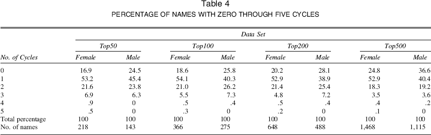
Next, I apply these definitions and the algorithm to identify cycles in the name choice context. Specifically, I set {M, τ, L} = {:00005, 4, 10} and analyze the time series of f_it in the data sets of interest.⁵ I perform my analysis on the Top50, Top100, Top200, and Top500 data sets and present the results in Table 4. Of the 361 Top50 names, more than 80% have experienced at least one cycle of popularity. Moreover, a significant fraction (30%) has gone through two or more cycles of popularity. This suggests the presence of recurring fashion cycles. In data sets with less popular names, the fraction of names with fashion cycles is lower, but still quite significant. For example, more than 75% of the 1,468 female names in the Top500 data set have gone through at least one cycle. Furthermore, over 20% of all names in Top50 have an amplitude of .005 or more, which implies that more than 10,000 babies were given these names at the peak of their popularity. For details on the empirical distributions of the length and amplitude of cycles, see the Web Appendix.

Note that if I set lower values of M, τ, and L, I would find more cycles in the data. By setting relatively high values of these parameters, I am setting a higher bar for classifying a bump or trough as a cycle. For a sensitivity analysis to varying τ and M, see the Web Appendix.

Table 4

PERCENTAGE OF NAMES WITH ZERO THROUGH FIVE CYCLES

No. of Cycles	Data Set
	Top50		Top100		Top200		Top500
	Female	Male	Female	Male	Female	Male	Female	Male
0	16.9	24.5	18.6	25.8	20.2	28.1	24.8	36.6
1	53.2	45.4	54.1	40.3	52.9	38.9	52.9	40.4
2	21.6	23.8	21.0	26.2	21.4	25.4	18.3	19.2
3	6.9	6.3	5.5	7.3	4.8	7.2	3.5	3.6
4	.9	0	.5	.4	.5	.4	.4	.2
5	.5	0	.3	0	.2	0	.1	0
Total percentage	100	100	100	100	100	100	100	100
No. of names	218	143	366	275	648	488	1,468	1,115

Notably, several names have gone through more than one cycle (for an example, see Figure 4). To better understand repeat cycles in names, I analyze the time it takes for cycles to repeat. I define “dormancy length” as the period between two popularity cycles in which the name is dormant or adoptions for the name are close to minimum. Formally,

Figure 4

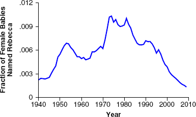
POPULARITY CURVE OF REBECCA

Definition 4:

Given two adjacent cycles C₁ = {x_i, x_j, x_k} and C₂ = {x₁, x_m, x_n}, such that |x_k – x₁| < d_t × Amp(C₂), where d_t < 1 is a dormancy threshold, the dormancy length is defined as 1 – k.

Table 5 provides the statistics for dormancy length when the dormancy threshold is defined as 10% (i.e., the change in values from the end of the first cycle to the beginning of the second cycle is less than 10% of the amplitude of the second cycle). For all four data sets (Top50, Top100, Top200, and Top500), the median dormancy period is between three and eight years. However, a large number of names also remain dormant for significant periods before experiencing a resurgence. For example, the 75th quartile of dormancy length for Top100 male names is 29. Furthermore, the dormancy periods are longer for female names compared with male names. Table 6 presents details on the main patterns of repeat cycles in the data. Different types of cyclical patterns are prevalent at varying frequencies. For instance, 13.6% of names in the Top100 data set have gone through a pattern, while 6.54% have gone through a pattern. Together, these findings provide strong support for the presence of cycles in data.

Table 5

DISTRIBUTION OF DORMANCY LENGTHS BETWEEN CYCLES

Quartile	Data Set
	Top50		Top100		Top200		Top500
	Female	Male	Female	Male	Female	Male	Female	Male
25	2	2	2	2	2	2	2	2
50	8	4	6	3	5	3	4	3
75	32	16	29	11	16	8	11	8

Notes: This table presents name dormancy lengths (in years) between cycles. The dormancy threshold is defined as 10% (i.e., the change in values from the end of the first cycle to the beginning of the second cycle is less than 10% of the amplitude of the second cycle).

Table 6

CYCLICAL PATTERNS IN THE DATA BY PERCENTAGE

Pattern Shape	Data Set
	Top50		Top100		Top200		Top500
	Female	Male	Female	Male	Female	Male	Female	Male
/or\	16.9	24.5	18.6	25.8	20.2	28.1	24.8	36.6
	26.1	22.4	24.6	16.4	18.2	13.3	12.1	8.5
	8.7	7.7	10.9	10.2	14.8	13.1	17.4	16.7
	3.7	1.4	3.3	1.1	3.1	1.8	4.6	3.9
	17.4	11.2	16.7	13.1	18.2	12.7	22.8	16.3
	13.3	17.5	11.5	16.4	10.0	14.8	8.0	10.0
	4.6	4.2	7.1	5.8	7.9	5.5	8.6	7.3
Other	9.3	11.1	7.3	11.2	7.6	10.7	1.7	.7
Total percentage	100	100	100	100	100	100	100	100
No. of names	218	143	366	275	648	488	1,468	1,115

Notes: Cycles were identified using the algorithmic definition of cycles.

A Statistical Framework for Identifying Cycles

In the previous section, I reported that the data present clear evidence of cycles. My efforts to identify and classify these cycles were algorithmic. I provided a specific definition of a cycle and identified patterns in the data that satisfied this definition. In this section, I establish the presence of cycles using statistical analyses. There are two main reasons for developing a statistical framework that goes beyond algorithmic methods. First, statistical methods are not influenced by user subjectivity, unlike the algorithmic methods, which require the values of τ, L, and M as user input. Second, statistical methods can include other explanatory variables that drive these cyclical patterns.

Fashion cycles differ from standard product life cycles (Day 1981; Levitt 1965) in two important ways. First, they can potentially reappear. Theory models of signaling-based fashions predict such recurring fashions (Corneo and Jeanne 1994), a prediction confirmed by casual observation (e.g., skinny jeans). Recall that even in this setting, a significant fraction of names go through multiple cycles of popularity. Second, fashion cycles have to be caused by social signaling. Both these properties must be satisfied for a cycle to be defined as a fashion cycle. For example, repeat cycles can occur without social signaling simply by being driven by a firm's marketing activities. Similarly, social signaling can occur in non-conspicuous arenas unrelated to fashion. Formally,

Definition 5:

An adoption curve is defined as a social signaling-based fashion cycle if (a) it satisfies statistical properties that can lead to repetitive cycles over sufficiently long periods and (b) the cycles (if they exist) are caused by social signaling—either wealth signaling or cultural capital signaling.

An empirical framework that aims to identify the presence and cause of fashion cycles in data must provide researchers tools to establish the two properties in Definition 5. In this section, I focus on the first aspect of the problem—identifying the presence of cycles in data using statistical tests. In the next section, I outline the second part of my framework and present tools to test whether the cycles are indeed caused by social signaling.

Conditional Monotonicity Property

Observe that name cycles are inverted V-shaped rather than inverted U-shaped curves. In this respect, they resemble stock market and real estate bubbles rather than standard product life cycle curves. Finance literature has shown that bubbles occur when consumers' utility and actions depend on their expectations and beliefs about others' valuation of the product rather than the inherent attributes of the product (Camerer 1989). In such settings, small changes in consumers' beliefs and expectations can cause large shifts in behavior. Because consumers' behavior in fashion markets is also driven by their beliefs about what other consumers consider fashionable (Yoganarasimhan 2012a), it is understandable that the popularity cycles of names follow similar patterns.

Note that unlike financial economists, who are interested in bubbles, I am interested in cycles. A bubble is defined as an autoregressive process that does not have a stable long-term mean. In contrast, a cycle is an autoregressive process that shows a clear cyclical behavior or generates an inverted V-shaped curve. Traditionally, the finance literature has used nonstationarity tests to identify bubbles in data (Charemza and Deadman 1995; Diba and Grossman 1988; Evans 1991). However, I show that nonstationarity alone is not sufficient to generate cycles and therefore provide a more precise framework for identifying cycles using the concept of “conditional monotonicity.”

Let the popularity of a conspicuously consumed product i evolve as an AR(p) process (i.e., an autoregressive process of order p) as follows:

y_{it} = \sum_{k = 1}^{p} ϕ_{k} y_{it - k} + [1 - \sum_{k = 1}^{p} ϕ_{k}] η_{i} + ε_{it},

(2)

where $| \sum_{k = 1}^{p} ϕ_{k} | \leq 1$ , y_it is a measure of product i's popularity in period t, $[1 - \sum_{k = 1}^{p} ϕ_{k}] η_{i}$ is an unobserved product fixed effect, and ∊_it is a mean-zero shock. The multiplier $[1 - \sum_{k = 1}^{p} ϕ_{k}]$ in front of η_i; ensures that the total effect of the unobservable in each period is always fixed at η_i.

This simple framework can be easily expanded to include other time-varying and time-invariant explanatory variables. Equation 2 can be rewritten as follows:

Φ_{p} (L) y_{it} = γ_{i} + ε_{it},

(3)

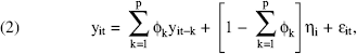
where Φ_p(L) = 1 – ϕ₁L – ϕ₂L² … – ϕ_pL^p, with L denoting the lag operator and $γ_{i} = [1 - \sum_{k = 1}^{p} ϕ_{k}] η_{i}$ . Depending on the parameter values, this process is either stationary or nonstationary.

An AR(p) process is stationary if all the roots of the polynomial Φ_p(L) lie outside the unit circle. Under these conditions, a shock to the system dissipates geometrically with time, and the resulting process is mean-reverting and stable. For example, if the popularity of name i follows a stationary process, then shocks to its popularity (e.g., election of a president with name i, the sudden fame of a celebrity with name i) will dissipate with time, and its popularity will soon return to its long-term average. (For detailed discussions on stationary time-series models, see Fuller [1995] and Dekimpe and Hanssens [1995].) In an AR(1) process, the stationarity condition boils down to |ϕ₁| < 1, and it can be written as y_it = ϕ₁y_it–1 + (1 – ϕ₁)η_i + ∊_it. Figure 5 shows an AR(1) process with ϕ₁ = .5 and η_i = 30. Note that this is a very stable process that oscillates around a constant mean of 30. The expectation of the tth realization of a stationary AR(p) series is a weighted mean of its last p realizations and the unobserved fixed effect η_i. Thus, every period, there is a constant pull toward the mean η_i, and this property makes a stationary process stable. Of course, an important implication of this stability is that a stationary process cannot give rise to popularity cycles significant in either time or magnitude.

Figure 5

AR(1) STATIONARY PROCESS WITH ϕ₁ = .5, η_i = 30

An AR(p) process is nonstationary if one or more of the roots of Φ_p(L) lies on the unit circle. When subjected to a shock, a nonstationary series does not revert to a constant mean, and its variance increases with time. If name choices are nonstationary, then shocks due to celebrities, politicians, and so on can cause long-term shifts in name popularity. An AR(1) process with ϕ₁ = 1 is nonstationary and is referred to as a random walk process. It can be written as y_it = y_it–1 + ∊_it ⇒ E(y_it) = y_it–1. Therefore, at any point in time, the process evolves randomly in one direction or the other. Although a random walk process is not mean-reverting, it also does not produce cycles of any significant magnitude, because its specification does not imply consecutive increases or decreases. Thus, nonstationary is not sufficient to generate cycles. Next, I define the conditional monotonicity property and describe its role in generating cycles. Let Δ be the first difference operator, such that Δy_it = y_it – y_it–1.

P₁: A nonstationary AR(p) process with roots 1, 1/c₁, 1/c₂,…, 1/c_p–1, where p ≥ 2 and 0 < c₁, c₂,…, c_p–1 ≤ 1, is conditionally monotonic in the following sense:

•

if $Π_{k = 1}^{p - 2} (1 - c_{k} L) Δ y_{i t - 1} \geq 0, t h e n E [Π_{k = 1}^{p - 2} (1 - c_{k} L) Δ y_{i t}] = c_{p - 1} Π_{k = 1}^{p - 2} (1 - c_{k} L) Δ y_{i t - 1} \geq 0.$

•

if $Π_{k = 1}^{p - 2} (1 - c_{k} L) Δ y_{i t - 1} \leq 0, t h e n E [Π_{k = 1}^{p - 2} (1 - c_{k} L) Δ y_{i t}] = c_{p - 1} Π_{k = 1}^{p - 2} (1 - c_{k} L) Δ y_{i t - 1} \leq 0.$

For a proof, see the Web Appendix.

According to P₁, in a conditionally monotonic AR(p) process, there is a lower bound on E(Δy_it) if the last p – 1 periods' changes satisfy the constraint $\prod_{k = 1}^{p - 2} (1 - c_{k} L) Δ y_{i t - 1} \geq 0$ .⁶ So, conditional on past lags, the current y_it is expected to be at least $\prod_{k = 1}^{p - 2} (1 - c_{k} L) Δ y_{i t - 1}$ , irrespective of η_i. Similarly, there is an upper bound on E(Δy_it) if $\prod_{k = 1}^{p - 2} (1 - c_{k} L) Δ y_{i t - 1} \leq 0$ . Note that these bounds are not dependent on η_i. In certain lower-order AR(p) processes, conditional monotonicity manifests itself as cycles.

When p = 2, there is an AR(2) process, and $Π_{k = 1}^{p - 2} = Π_{k = 1}^{0} = 1$ by definition.

Next, I demonstrate the implications of conditional monotonicity for an AR(2) process (for a general proof for an AR(p) process, see the Web Appendix). Consider a nonstationary AR(2) process of the form y_it = (1 + c₁)y_it–1 – c₁y_it–2 + γ_i + ∊_it, where 0 < c₁ ≤ 1 and $γ_{i} = (1 - \sum_{k = 1}^{2} ϕ_{k}) η_{i} = {1 - [(1 + c_{1}) - c_{1}]} η_{i} = 0$ . Note that this process satisfies the requirements for conditional monotonicity, because its two roots are 1 and 1/c₁, where 0 < c₁ ≤ 1. This series can be rewritten as y_it = y_it–1 + c₁Δy_it–1 + ∊_it. When this series is on an increasing trend, it has a tendency to keep increasing because E(y_it) = y_it–1 + c₁Δy_it–1 > y_it–1 when Δy_it–1 > 0. That is, conditional on an increase in the last period (Δy_it–1 > 0), the series continues to increase in expectation. Similarly, when this series is on a decreasing trend, it has a tendency to keep decreasing because E(y_it) = y_it–1 + c₁Δy_it–1 < y_it–1 when Δy_it–1 < 0. That is, conditional on a past decrease (Δy_it–1 < 0), the series continues to decrease in expectation. In data, this property manifests itself as periods of consecutive increase followed by periods of consecutive decrease—a pattern that can be interpreted as cycles. Thus, the presence of fashion cycles in an AR(2) process can be established by showing that the underlying process is conditionally monotonic. As an illustration, see Figure 6, which shows the presence of cycles in the conditionally monotonic process defined by y_it = 1.5y_it–1 – .5y_it–2 + ∊_it and η_i = 30.

Figure 6

AR(2) CONDITIONALLY MONOTONIC PROCESS WITH ϕ₁ = 1.5, ϕ₂ = –.5, η_i = 30

Note that nonstationarity is necessary, but not sufficient, for conditional monotonicity. Nonstationarity is necessary because in stationary processes, the conditional expectation E(y_it) remains dependent on η_i, which precludes making any general statements on the relationship between E(y_it) and its past (p – 1) lags. For example, consider the stationary AR(2) process y_it = ϕ₁y_it–1 + ϕ₂y_it–2 + γ_i + ∊_it, where $γ_{i} = (1 - \sum_{k = 1}^{2} ϕ_{k}) η_{i} \neq 0$ . In this case, E(y_it) = ϕ₁y_it–1 + ϕ₂y_it–2 + γ_i. Even when this process is on an increasing trend (Δy_it–1 > 0), I cannot make the general claim that E(y_it) > y_it–1, because E(y_it) depends on η_i. Therefore, nonstationarity is a necessary prerequisite for conditional monotonicity. However, nonstationarity is not sufficient to induce consecutive periods of increase or decrease. For example, consider the nonstationary AR(2) process y_it = .5y_it–1 + .5y_it–2 + ∊_it ⇒ y_it(1 – L)(1 + .5L) = ∊_it. This process is not conditionally monotonic, because one of its roots is −2 (i.e., c₁ = -.5 < 0). Note that this does not give rise to consecutive increases or decreases because E(y_it) = .5 (y_it–1 + y_it–2) < y_it–1 when Δy_it–1 > 0. Thus, conditional monotonicity, beyond nonstationarity, is needed to establish the presence of cycles in the data.

Finally, a conditionally monotonic process needs to be observed for sufficiently long periods of time to generate cycles. Although the property is defined over the change in the y_it from the last period, such changes need to be observed for a long-enough period to observe a full cycle or multiple cycles (as in Figure 6).

Application: Identifying Cycles in the Choice of Given Names

Model

Next, I expand Equation 2 to suit the specific context as follows:

y_{it} = const . + \sum_{k = 1}^{p} ϕ_{k} y_{it - k} + {αx}_{it} + {βz}_{i} + γ_{i} + ε_{it},

(4)

where y_it denotes n_it, number of babies given name i in period t. This is modeled as a function of the following:

The last p lags of i's popularity. This captures the past trends in name i's popularity that can affect adoption by current parents.

X_it, time-varying factors that affect i's popularity. Here, x_it consists of the number of babies of sex s_i born in year t and time dummies.

Z_i, the time-invariant attributes of name i that affect its popularity: length, sex, and number of Biblical mentions.

A name fixed effect $γ_{i} = [1 - \sum_{k = 1}^{p} ϕ_{k}] η_{i}$ , which comprises time-invariant unobservables that affect name i's popularity, such as its historical relevance, symbolism, and meaning.

A mean-zero shock ∊_it that captures shocks to a name's popularity. This can stem from a variety of factors, including but not limited to the rise or fall of celebrities, entertainers, and book characters.

Furthermore, I make the following assumptions about the model:

Assumption 1:

E(∊_it) = (γ_i × ∊_it) = E(∊_it × ∊_ik) = 0 ∀ i, t, k ≠ t. I follow the familiar error components structure (i.e., en is mean zero and uncorrected to γ_i for all i, t). ∊_it is allowed to be heteroskedastic but assumed to be serially uncorrected. Because this is an important and strong assumption, I test its validity after estimating the model using the Arellano-Bond (2) test.

Assumption 2:

E(x_ik × ∊_it)=E(x_ik × γ_i)=E(z_i × ∊_it)=E(z_i ×γ_i) = 0 ∀ i, k, t.

The time-invariant attributes of a name are assumed to be uncorrelated to both ∊_it and γ_i. x_it is assumed to be uncorrected to γ_i because the long-term mean of any name i is unlikely to be correlated with the total births of either sex in year t. Moreover, because the decision to have a child is unlikely to be influenced by shocks in the popularity of a specific name i, there is no reason to expect ∊_it to be correlated to past, current, or future births.

Assumption 2 is specific to this context. In a different context, in which explanatory variables are predetermined or potentially endogenous, it can be easily relaxed (see the “Statistical Framework for Analyzing the Drivers of Fashion” section).

Although both x_it and z_i are uncorrelated to the shock and the fixed effect, the same cannot be said of the lagged dependent variables—the dynamics of the model imply an inherent correlation between the lagged dependent variables (y_it–1, …, y_it–k) and the unobserved heterogeneity γ_i if γ_i ≠ 0. Moreover, ys and ∊s are correlated by definition. Because the current error term affects both current and future popularity, ⇒ E(y_ik × ∊_it) ≠ 0 if k ≥ t. However, past popularity remains unaffected by future shocks ⇒ E(y_ik × ∊_it) = 0 if k < t.

Estimation

I rewrite Equation 4 as follows and use this formulation in the subsequent analyses:

y_{it} = const . + {μy}_{it - 1} + \sum_{k = 1}^{p - 1} θ_{k} Δ y_{it - k} + {αx}_{it} + {βz}_{i} + γ_{i} + ε_{it},

(5)

where $μ = \sum_{k = 1}^{p} ϕ_{k}$ and $θ_{k} = - \sum_{j = k + 1}^{p} ϕ_{k}$ .

If all the panels in the data set follow a nonstationary process, then $[1 - \sum_{k = 1}^{p} ϕ_{k}] η_{i} = 0 \Rightarrow γ_{i} = 0 \forall i$ . In such cases, the endogeneity bias due to the correlation between the lagged dependent variables (y_it–1,…, Y_it–k) and the name fixed effect η_i is not an issue and, in theory, Equation 4 can be consistently estimated using pooled ordinary least squares (OLS) (Bond, Nauges, and Windmeijer 2002). However, if the nonstationarity assumption is violated even for a few panels, pooled OLS estimates are inconsistent. Moreover, in the next section, I consider models with endogenous time-varying variables (x_it), and such models cannot be estimated using pooled OLS. Therefore, I avoid pooled OLS and look for estimators that can accommodate endogenous variables and are robust to deviations from nonstationarity.

The two commonly used methods of estimating panel data models, random-effects estimation and fixed-effects estimation, cannot be used in a dynamic setting. The former requires explanatory variables to be strictly exogenous to the fixed effect γ_i, an untenable assumption if some panels are indeed stationary. The latter allows for correlation between γ_i and explanatory variables, but because it uses a within transformation, it requires all time-varying variables to be strictly exogenous to ∊_it. This is impossible in a dynamic setting with finite T (Nickell 1981). Although theoretically, I can solve this problem by finding external instruments, it is difficult to find variables that affect lagged name popularity but not current name popularity. Therefore, I turn to the GMM-style estimators of dynamic panel data models that exploit the lags and lagged differences of explanatory variables as instruments (Blundell and Bond 1998). This methodology has been successfully applied by researchers in a wide variety of fields in marketing and economics (for details, see Acemoglu and Robinson 2001; Clark, Doraszelski, and Draganska 2009; Durlauf, Johnson, and Temple 2005; Shriver 2015; Yoganarasimhan 2012b). I briefly outline the method next.

System GMM estimator

First, consider the first-difference of Equation 5.

Δ y_{it} = μ Δ y_{it - 1} + \sum_{k = 1}^{p - 1} θ_{k} Δ^{2} y_{it - k} + α Δ x_{it} + Δ ε_{it} .

(6)

Note that first-differencing has eliminated the fixed effect γ_i, thereby eliminating the potential correlation between the lagged dependent variables and γ_i. However, first-differencing introduces another kind of bias. Now, the error term Δ∊_it is correlated with the explanatory variable Δy_it–1 through the error term ∊_it–1. However, it is easy to show that lags and lagged differences of y_it from time period t – 2 and earlier are uncorrelated to Δ∊_it and can therefore function as instruments for Δy_it–1 and Δ²y_ik. In addition, because Δx_it is uncorrelated with Δ∊_it, it can instrument for itself. Thus, I specify the following sets of moment conditions for Equation 6:

E (y_{ip} \times Δ ε_{it}) = 0 \forall p \leq t - 2,

(7)

E (Δ y_{ip} \times Δ ε_{it}) = 0 \forall p \leq t - 2, and

(8)

E (Δ x_{it} \times Δ ε_{it}) = 0 \forall t .

(9)

In theory, these moments are sufficient to identify ϕ_k and α as long as the process is not first-order nonstationary (Blundell and Bond 1998). However, a priori, it is not clear whether these moment conditions are sufficient for identification in the current context. So, following Blundell and Bond (1998), I also consider moment conditions for the level Equation 5.

E [Δ y_{iq} \times (γ_{i} + ε_{it})] = 0 \forall q \leq t - 1,

(10)

E [Δ^{2} y_{iq} \times (γ_{i} + ε_{it})] = 0 \forall q \leq t - 1,

(11)

E [x_{it} \times (γ_{i} + ε_{it})] = 0, and

(12)

E [z_{i} \times (γ_{i} + ε_{it})] = 0

(13)

x_it and z_i can instrument for themselves because they are uncorrelated to both γ_i and ∊_it. Lagged differences of y_it from period t – 1 and earlier can be used as instruments for y_it–1 and Δy_it–k. The moment conditions in Equations 10 and 11 hold irrespective of the stationarity properties of the process. They require only the initial deviations of the dependent variable to be independent of its long-term average, which is a reasonable assumption in most settings, including the current setting.

Stacking the moments results in a system GMM estimator that provides consistent estimates regardless of the stationarity properties of the process. I employ a two-step version of the estimator because it is robust to panel-specific heteroskedasticity and increases efficiency. However, the standard errors of the two-step GMM estimator are known to be biased. Windmeijer (2005) proposes a correction for this bias, and I follow his method to obtain robust standard errors.

Serial correlation and lagged dependent variables

A key assumption in the method in the previous subsection is that the error terms are not serially correlated. Serial correlation is problematic for two reasons. First, in the presence of serial correlation, the restrictions that I apply break down. For example, consider a scenario in which errors follow a moving average (1) process such that ∊_it = ρ∊_it–1 + u_it, where E(u_it) = 0 and E(u_it × u_ik) = 0 ∀ k ≠ t. Then, for q = t – 1, Equation 10 can be expanded as E[Δy_it–1 × (γ_i + ρ∊_it–1)] = 0. However, this moment condition is invalid because Δy_it–1 is correlated with ∊_it–1. Similarly, the moment conditions in Equations 7, 8, and 11 also fail to hold in the presence of serial correlation. Second, the absence of serial correlation confirms the absence of omitted variable biases (for a detailed discussion on this issue, see the subsection “Controlling for Other Factors that Affect Name Choice”). Therefore, for all the models estimated herein, I test the validity of the instruments and the absence of omitted variable bias using the Arellano-Bond (1991) test for serial correlation.

Results and discussion

I estimate the model on the four data sets of interest (Top50, Top100, Top200, and Top500) and present the results in Table 8. The instruments for each of the level and differenced equations appear in the last four rows of the table. The GMM refers to the instruments generated from the lagged dependent variables, and standard refers to exogenous variables that instrument for themselves.

In all the models, I find that the coefficient of Δy_it–2 is insignificant, implying that the process is AR(2). Thus, Equation 5 can be written as

y_{it} = const . + {μy}_{it - 1} + θ_{1} Δ y_{it - 1} + {αx}_{it} + {βz}_{i} + γ_{i} + ε_{it} .

(14)

This process satisfies the conditional monotonicity property if and only if μ = 1 and 0 < θ₁ ≤ 1. Under these conditions, the two roots of the process are 1 and 1/θ₁, where 0 < θ₁ ≤ 1. Thus, for all the four models, I test the following two hypotheses:

H₁: μ = 1.

H₂: $θ_{1} = {\bar{θ}}_{1}$ , where ${\bar{θ}}_{1}$ is a positive constant such that $0 < {\bar{θ}}_{1} \leq 1$ .

Table 8 shows the results from the hypothesis tests. First, for all four models, I cannot reject the null of H₁ (μ = 1). This suggests that the data-generating process is nonstationary and contains a unit root. Second, in all the models, I cannot reject the null of H₂ (θ₁ = .47).⁷ Together, these results present clear evidence for the existence of cycles in the data because they demonstrate the conditional monotonicity of the underlying process.

In principle, this could be any positive θ₁ between 0 and 1. Because my estimates show that θ₁ ≈ .47, I use this specific number to show that the hypothesis that θ₁ is positive and less than 1 cannot be rejected.

The Arellano-Bond test confirms that the model is not misspecified; I cannot reject the null hypothesis of no second-order serial correlation in first-differenced error terms (i.e., the tests present no evidence of serial correlation). This establishes the validity of my moment conditions and confirms the absence of omitted variable biases. Nevertheless, I include time-period dummies in all models. They control for unobserved time-varying variables such as education, income, urbanization, and religious preferences, which may affect name choice.

In all the models, the coefficient of z; is insignificant. This is understandable because in a truly nonstationary model, the impact of time-invariant observed attributes should also be zero, just as the impact of the time-invariant unobserved attributes is zero. Recall that $γ_{i} = (1 - \sum_{k = 1}^{p} ϕ_{k}) η_{i} = 0$ because $(1 - \sum_{k = 1}^{p} ϕ_{k}) = 0$ . Similarly, β can be expressed as $β = \hat{β} (1 - \sum_{k = 1}^{p} ϕ_{k}) = 0$ .

The results are robust to variations in model specification and data used. When I estimate the model with f_it (the fraction of babies given name i in period t) as the dependent variable instead of n_it (number of babies given name i in period t), the qualitative results remain unchanged. Similarly, the results are robust to the following changes in the data: (1) inclusion of all the names that have been in top 1,000 at least once (this data set can be referred to as Top 1000), (2) inclusion of a set of randomly picked names to the existing data sets, and (3) inclusion of observations prior to 1940 (i.e., analyzing all the data from 1880 to 2009 instead of focusing on the data from 1940 to 2009).

Statistical Framework for Analyzing the Drivers of Fashion

The previous two sections show that there is both algorithmic and statistical evidence for the existence of popularity cycles of large magnitudes in the data. In this section, using state-level variation in economic and cultural capital, I examine whether these cycles are consistent with one of the two signaling theories of fashion: (1) fashion as a signal of wealth and (2) fashion as a signal of cultural capital. I also consider and rule out a series of alternative explanations.

I begin with a visual example using the popularity curve of the name Heather (Figure 7). Panel A shows Heather's popularity in the three most and three least educated states. It is clear that Heather became popular in the more educated states (Massachusetts, Connecticut, and Colorado) before it took off in the least educated ones (West Virginia, Arkansas, and Mississippi). Similarly, note that it begins dropping in popularity in the highly educated states first. However, no such patterns appear in Panel B, which shows Heather's popularity cycles in the three most and three least wealthy states. This pattern also repeats in more recently popular names such as Sophia (Figure 8). Taken together, these patterns are suggestive evidence in support of the cultural capital theory. However, visual evidence from a few names is not conclusive, so I examine the data further for model-free patterns.

Figure 7

POPULARITY OF HEATHER IN THE MOST AND LEAST EDUCATED STATES AND THE MOST AND LEAST WEALTHY STATES

Figure 8

POPULARITY OF SOPHIA IN THREE OF THE MOST AND LEAST EDUCATED STATES AND THE MOST AND LEAST WEALTHY STATES

Preliminary examination of the data indicates that there are significant differences in when a name takes off and peaks across states. Table 7 compares the relative order of peaking in Colorado (high-cultural capital state) and West Virginia (low-cultural capital state). In the Top500 names, 71.33% of the names peak in Colorado before West Virginia (i.e., names tend to take off and peak in high-cultural capital states before low-cultural capital states). Nevertheless, even this finding is not conclusive because it does not control for other factors that affect name choice. So, hereinafter, I focus on empirical analysis.

Table 7

RELATIVE ORDERING OF WHEN NAMES PEAK IN COLORADO AND WEST VIRGINIA BASED ON THE ALGORITHMIC DETECTION OF CYCLES

	Data Set
	Top50		Top100		Top200		Top500
	Female	Male	Female	Male	Female	Male	Female	Male
CO peaks first	92	62	159	73	283	242	668	489
WV peaks first	54	0	87	0	151	0	340	125

Table 8

ESTIMATION RESULTS AND CONDITIONAL MONTONICITY TESTS

Variable		Model M1		Model M2		Model M3		Model M4
Variable		Estimate	SE	Estimate	SE	Estimate	SE	Estimate	SE
L.Number	n_it–1	.9875^***	.0488	.9893^***	.0197	.9956^***	.0062	.9958^***	.0042
L.Δ	Number Δn_it–1	.4785^**	.2004	.4739^***	.1348	.4708^***	.1154	.4675^***	.0728
L2.Δ	Number Δn_it–2	.0630	.1684	.0580	.1540	.0479	.0902	.0451	.0582
Length	l_i	10.849	18.661	3.4902	37.249	.8112	3.4730	.1787	.3737
Bible	bib_i	.3207	1.7048	.1634	.8375	.0570	.1353	.0083	.0418
Sex	s_i	–161.0	317.13	–13.31	2,887.0	–3.2654	187.19	2.1934	48.589
Total babies	$Γ_{s_{i} t}$	–5.5e-4	.0011	–4.5e-6	.0133	–8.7e-7	.0009	1.5e-5	.0002
Const.	k	873.80	3,283.2	31.656	25,551	29.084	2,346.8	–19.81	353.94
Time dummies		Yes		Yes		Yes		Yes
Conditional Monotonicity Test
H₁: μ = 1		Do not reject		Do not reject		Do not reject		Do not reject
z-statistic (p-value)		–.256 (.401)		–.543 (.295)		–.710 (.239)		–.970 (.166)
H₂: θ₁ = :47		Do not reject		Do not reject		Do not reject		Do not reject
z-statistic (p-value)		.042 (.516)		.029 (.512)		.007 (.504)		–.034 (.488)
AR–Bond (2) test		Do not reject		Do not reject		Do not reject		Do not reject
Test statistic (p-value)		–.825 (.409)		–.816 (.414)		–1.126 (.260)		–1.524 (.128)
Correlation(y, ŷ)		.9962		.9963		.9964		.9966
Root mean standard error		887.9		691.3		533.2		358.5
Mean absolute error		392.2		268.8		178.5		92.88
Diff. equation	GMM	L(2/3).{n_it, Δn_it}		L(2/3).{n_it, Δn_it}		L(2/3).{n_it, Δn_it}		L(2/3).{n_it, Δn_it}
Instrument	Standard	$Δ Γ_{s_{i} t}$		$Δ Γ_{s_{i} t}$		$Δ Γ_{s_{i} t}$		$Δ Γ_{s_{i} t}$
Level equation	GMM	LΔ{n_it, Δn_it}		LΔ{n_it, Δn_it}		LΔ{n_it, Δn_it}		LΔ{n_it, Δn_it}
Instrument	Standard	$s_{i}, 1_{i}, u_{i}, Γ_{s_{i} t}$		$s_{i}, 1_{i}, u_{i}, Γ_{s_{i} t}$		$s_{i}, 1_{i}, u_{i}, Γ_{s_{i} t}$		$s_{i}, 1_{i}, Γ_{s_{i} t}$
No. of names, years		361, 67		641, 67		1,136, 67		2,583, 67
Data set used		Top50		Top100		Top200		Top500

p ≤ .1.

p ≤ .05.

***

p ≤ .01.

Notes: The dependent variable is n_it.

To confirm that the cycles in the data are consistent with social signaling, my empirical tests should confirm the following two statements:

•

The high types are the first to adopt a name, followed by low types. Similarly, high types are the first to abandon the name, followed by low types (i.e., the rate of adoption is higher among the high types at the beginning of the cycle, whereas the opposite is true at the end of cycle).

•

Adoption by high types has a positive impact on the adoption of the general population, whereas adoption by low types has a negative impact on the adoption of the general population.

In these statements, high types = wealthy and low types = poor if the wealth signaling theory is true, and high types = cultured and low types = uncultured if the cultural capital signaling theory is true. The following subsections present two models that test the validity of each of these statements.

A potential issue with using state-level data to make inferences on individual behavior is aggregation bias (Blundell and Stoker 2005; Stoker 1993). For an explanation of how an individual-level model aggregates to the state-level models employed in this section, see the Web Appendix.⁸

States serve as the lowest level of geography in the data. Thus, all models in this section are specified at the state level. In a study on installed base effects in hybrid adoptions, Narayanan and Nair (2012) find that social effects tend to be stronger at lower geographical aggregations. So, this study's use of a relatively high level of aggregation should, if anything, reduce the likelihood of finding evidence in favor of social signaling.

Interacting Wealth and Cultural Capital with Past Adoptions

Model

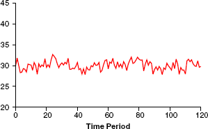
I expand the model of name popularity to the state level as follows:

\begin{matrix} y_{ijt} & = & const . + \sum_{k = 1}^{p} ϕ_{k} y_{ijt - k} + λ_{w} w_{jt} + λ_{c} c_{jt} + δ_{w} w_{jt} y_{it - 1} \\ + δ_{c} c_{jt} y_{it - 1} + α_{1} x_{ijt}^{1} + α_{2} x_{ijt}^{2} + {βz}_{i} + γ_{ij} + ε_{ijt}, \end{matrix}

(15)

where

•

y_ijt = n_ijt, which is the popularity of name i in state j at time t;

•

W_jt and c_jt are metrics of wealth and cultural capital of state j in period t;

•

w_jty_it–1 and c_jty_it–1 capture the interaction between the lag of the total country level adoption of name i and the wealth and cultural capital of state j, respectively;

•

$x_{i j t}^{1}$ is an endogenous time-varying factor that affects name popularity, such as past lags of the number of babies given name i at the national level (denoted as y_it–1, y_it–2, etc.);

•

$x_{i j t}^{2}$ is an exogenous time-varying factor that affects name popularity, such as the total number of babies born in state j in period t and time dummies;

•

z_i is a time-invariant attribute of the name (discussed in the “Model” subsection);

•

$γ_{i j} = [1 - \sum_{k = 1}^{p} ϕ_{k}] η_{i j}$ is an unobserved name-state fixed effect that controls for the mean unobserved state-level preference for name i; and

•

ε_ijt is an i.i.d mean-zero time- and state-varying shock that affects the popularity of name i in state j. It captures differential exposure and other random effects (e.g., the television show with a lead character named i may randomly be aired in one market before another, a local news item may mention name i in state j at time t).

This model can be augmented to include state-time dummies. However, I found no significant effects for such dummies, so I omit them here.

y_it–1k terms are endogenous because y_it–k is a function of y_ijt–k, which in turn is a function of γ_ij ⇒ E(y_it–k × γ_ij) ≠ 0. Because the interaction terms w_jty_it–1 and c_jty_it–1 are functions of y_it–1, I treat them as endogenous too. I modify the previous moment conditions to accommodate these changes and ensure that these correlations are not violated in the moment conditions. To avoid repetition, the estimation strategy is not described again. However, for each model estimated, I list the set of instruments for the level and first-differenced equations when presenting the results.

Results and Discussion

Model N1 in Table 9 presents the results from the estimating the model on the Top50 data set. Next, I discuss the estimates from this model (for robustness checks, see the “Robustness Checks” subsection.⁹

Recall that name data are left-truncated at 5. At the state level, in Top50 names, 22.01% of the data are zero; in Top100, 29.54% of the data are zero; in Top200, 41.54% of the data are zero. I cannot tell how many of these are truly zeroes and how many are values less than five. If I include less popular names, a significant fraction of these zeroes are likely to come from truncation. Truncation can adversely affect the quality and significance of the estimates. Thus, to keep the estimates clean, I avoid less popular names and confine my analysis to the Top50 and Top100 data sets.

Table 9

IMPACT OF ADOPTION BY HIGH AND LOW TYPES

Variable		Model N1		Model P1		Model P2
Variable		Estimate	SE	Estimate	SE	Estimate	SE
Lagged dependent variable	n_ijt–1	.9967^***	.2547 × 10^–2	.1006 × 10¹^***	.4257 × 10^–2	.9965^***	.1970 × 10^–2
	Δn_ijt–1	.6498 × 10^–1^***	.1418 × 10^–1	.6911 × 10^–1^***	.2291 × 10^–1	.6383 × 10^–1^***	.8756 × 10^–2
	Δn_ijt–2	.1484^***	.8726 × 10^–2	.1511^***	.2151 × 10^–1	.1499^***	.7894 × 10^–2
	Δn_ijt–3	.1210^***	.5229 × 10^–2	.1171^***	.8039 × 10^–2	.1216^***	.4859 × 10^–2
	Δn_ijt–4	.8465 × 10^–1^***	.6763 × 10^–2	.8363 × 10^–1^***	.1602 × 10^–1	.8450 × 10^–1^***	.5837 × 10^–2
Name characteristic	l_i	.1630^***	.2888 × 10^–1	.2386^***	.4218 × 10^–1	.11081^***	.2965 × 10^–1
	bib_i	.5866 × 10^–2^***	.2144 × 10^–2	.1031 × 10^–1^***	.2202 × 10^–2	.46011 × 10^–2^***	.2211 × 10^–2
	s_i	–.5408^***	.7784 × 10^–1	–.7938^***	.1151	–.4897^***	.7873 × 10^–1
Cultural capital	c_jt	.7749 × 10^–1^***	.2965 × 10^–1			.8071 × 10^–1^***	.2752 × 10^–1
	c_jt.n_it–1	–.2780 × 10^–4^***	.7630 × 10^–5			–.2740 × 10^–4^**	.6950 × 10^–5
	$Γ_{s_{i} j t}$			.2076 × 10³^***	.4423 × 10²	.1465 × 10³^***	.4699 × 10²
Economic capital	w_jt	–.2757 × 10^–1^***	.1656 × 10^–2			–.2821 × 10^–1^***	.1621 × 10^–2
	w_jt.n_it–1	.9110 × 10^–5^***	.3780 × 10^–6			.9290 × 10^–5^***	.3660 × 10^–6
	$d_{i t - 1}^{w}$			.5278 × 10²	.7038 × 10²	.2448 × 10³^***	.5875 × 10²
Other	n_it–1	.9978 × 10^–3^***	.2708 × 10^–3	.4446 × 10^–2^***	.2577 × 10^–3	.9712 × 10^–3^***	.2059 × 10^–3
	n_it–2	–.5499 × 10^–2^***	.2197 × 10^–3	–.4874 × 10^–2^***	.2627 × 10^–3	–.5523 × 10^–2^***	.1509 × 10^–3
	$Γ_{s j t}$	.4880 × 10^–5	.4830 × 10^–5	–.1660 × 10^–4^**	.8390 × 10^–5	.5430 × 10^–5	.4090 × 10^–5
	Const.	.1335 × 10²^***	.8790	.9494^***	.3415	.1379 × 10²^***	.8359
AR-Bond (2) test		Do not reject		Do not reject		Do not reject
Test statistic (p-value)		–.8918 (.3725)		–.5381 (.5905)		–.8741 (.3821)
Diff. equation	GMM	L(2/4)[n_ijt,Δn_ijt,n_it,c_jt.n_it–1,w_jt.n_it–1]		L(2/4) [n_ijt,Δn_ijt,n_it]		L(2/4) [n_ijt,Δn_ijt,n_it,c_jt.n_it–1,w_jt.n_it–1]
Instrument	Standard	$Δ [Γ_{s_{i} j t}, c_{j t}, w_{j t}]$		$Δ [Γ_{s_{i} j t}, d_{i t - 1}^{c}, d_{i t - 1}^{w}]$		$Δ [Γ_{s_{i} j t}, c_{j t}, w_{j t}, d_{i t - 1}^{c}, d_{i t - 1}^{w}]$
Level equation	GMM	L2 Δ[n_ijt,Δn_ijt,n_it,c_jt.n_it–1,w_jt.n_it–1]		L2Δ[n_ijt,Δn_ijt,n_it]		L2Δ[n_ijt,Δn_ijt,n_it,c_jt.n_it–1,w_jt.n_it–1]
Instrument	Standard	$[s_{i}, 1_{i}, b i b_{i}, Γ_{s_{i} j t}, c_{j t}, w_{j t}]$		$[s_{i}, 1_{i}, b i b_{i}, Γ_{s_{i} j t}, d_{i t - 1}^{c}, d_{i t - 1}^{w}]$		$[s_{i}, 1_{i}, b i b_{i}, Γ_{s_{i} j t}, c_{j t}, w_{j t}, d_{i t - 1}^{c}, d_{i t - 1}^{w}]$
No. of names, states, years		361, 50, 35		361, 50, 35		361, 50, 34
Data set used		Top50		Top50		Top50

p ≤ .1.

p ≤ .05.

***

p ≤ .01.

Notes: The dependent variable is n_ijt.

In Model N1, the mean effect of c_jt is positive, and its interaction with past country level adoption c_jt × y_it–1 is negative. So the total effect of c_jt is c_jt (7:749 × 10^–2 – 2:780 × 10^–5 × y_it–1). Recall that c_jt is positive for states with high education and negative for states with low education (Table 3). For low values of y_it–1 (≈ y_it–1 < 2,787), the overall impact of c_jt is increasing with education. Thus, at low values of y_it–1, the impact of education is increasingly positive for states with education higher than the national average (c_jt > 0) and increasingly negative for states with education lower than the national average (c_jt < 0). This suggests that high-education states are more likely, and low-education states are less likely, to adopt a name at the early stages of the cycle (when its countrywide adoption is low). Conversely, for high values of y_it–1 (approximately y_it–1 > 2,787), the opposite is true. Here, the overall impact of c_jt is increasingly negative for high-education states (c_jt > 0) and increasingly positive for states with low education (c_jt < 0). That is, high-education states are more likely to abandon a name as it becomes very popular, and the rate of abandonment increases with education. In contrast, low-education states are more likely to adopt a name as it becomes very popular, and this rate of adoption increases as education levels decrease.

The effect of the wealth metric, w_jt, is the opposite of that of education—the mean effect of w_jt is negative, while its interaction with past country-level adoption w_jt × y_it–1 is positive. This suggests that, after controlling for cultural capital, name cycles begin in the less wealthy states and then spread to the wealthier ones. Thus, the results do not support wealth signaling theory but are consistent with the cultural capital theory.

Controlling for other Factors that Affect Name Choice

Next, I explain how the model controls for other factors that affect name choice, as discussed previously. These include name attributes, familial and religious reasons, and celebrity names.

Name attributes

I control for time-invariant name attributes using observed variables such as length, number of Biblical mentions, sex, and an unobserved state-name fixed effect γ_ij. γ_ij captures state j's preference for the name as well as the name's origin, symbolism, ease of pronunciation, and so on. The inherent unobserved attractiveness of a name in a state can change over time and cause state-level trends in its popularity. Such trends are captured through lagged dependent variables (y_ijt–k).

Familial and religious reasons and assimilation/differentiation incentives

Familial and religious reasons as well as assimilation/differentiation incentives can be grouped under the heading of peer effects because they capture the impact of previous adoptions by others of same ethnicity, familial background, or religion on one's own adoption of a name (Nair, Manchanda, and Bhatia 2010; Shriver, Nair, and Hofstetter 2013). They are captured using lagged dependent variables. If lags are insufficient controls, the model would suffer from serial correlation, which is not so in this case.¹⁰ Thus, in all models estimated, I take care to add enough lags of past adoption on the right-hand side to control for such time-varying name-specific effects. I verify the adequacy of these controls using the Arellano-Bond test, which confirms the absence of serial correlation.

A simple example illustrates the reasoning behind this finding. Consider a scenario in which parents' choices are influenced (among other things) by their need to fit in with a certain ethnic group. To this end, they may want to pick names that are currently popular in this group. Formally, let r_ijt–1 denote the number of babies from the ethnic group given name i in state j in period t – 1 and suppose that this number affects i's popularity in state j in period t. In the model, r_ijt–1 is indirectly controlled for through y_ijt–1 (which is a function of r_ijt–1), which is an adequate control. If it were not adequate, r_ijt–1 would be a true omitted variable that would appear in the error term as follows: ∊_ijt, = δr_ijt–1 + u_ijt, where E(u_ijt) = E(u_ijt × u_ikt) = 0∀t, k ≠ t. Moreover, because the number of parents from the ethnic group choosing name i in period t – 1 is likely to be highly correlated to the number of parents from this group choosing name i at period t – 2, r_ijt–1 can be expressed as r_ijt–1 = ζr_ijt–2 + ν_ijt–1, where E(ν_ijt) = E(ν_ijt × ν_ijk) = 0 ∀ t, k ≠ t. In that case, E(∊_ijt × ∊_ijt–1) = E[(δr_ijt–1 + u_ijt) × (δr_ijt–2 + u_jit–1)] = δ²(r_ijt–1 × r_ijt–2) = δ²ζ ≠ 0. Thus, if the lags of y_ijt–1 do not sufficiently control for name-specific time-varying factors that affect name popularity, the model would suffer from serial correlation.

Celebrity names

As discussed previously, a popular lay theory of name adoption is based on celebrity adoption. Although prior research has refuted this theory (Lieberson, 2000), in this subsection I explain how the model controls for celebrity adoptions.

First, the impact of newly popular celebrities on naming decisions is captured through time-varying error terms (Eyt). Once a celebrity is well-known, the lagged dependent variables account for the past unobserved effect of the celebrity's name on parents' choice (through either awareness of the name or adoptions by other parents). Again, the lack of serial correlation in the error terms ensures that these unobserved effects are adequately controlled for. More importantly, a celebrity-based theory cannot account for the differential rate of adoption (or abandonment) among different subsets of parents.

Robustness Checks

I conducted many checks to validate the robustness of the results and outline the key ones in this subsection. First, I reestimated the model with the Top100 data set to confirm that the qualitative results remain the same (see Model N2 in the Web Appendix). Next, according to Berry, Fording, and Hanson (2000), the BFH index does not sufficiently normalize the cost of living for Alaska, making it look wealthier than it really is. Therefore, I excluded it and reran the analysis to confirm that the results are similar to the previous ones (see Model N3 in the Web Appendix).

Impact of Adoption by States with the Highest and Lowest Cultural and Economic Capital

So far, the analysis has been restricted to analyzing the adoption patterns of a name within a state and relating it to the education and income of its residents. However, a given state may also be influenced by the adoption (or abandonment) of a name in high-/low-culture (or high-/low-income) states. This influence can help in the spread of names across states and explains the rise and fall of fashion cycles (see the “Deconstructing a Fashion Cycle” subsection). Next, I specify and estimate a model in which I examine the impact of the difference in the adoption levels in the most and least cultured (and wealthy) states on the rest of the states.

Model and results

Let ${j_{1 t}^{w}, j_{2 t}^{w}, j_{3 t}^{w}}$ and ${j_{4 t}^{w}, j_{5 t}^{w}, j_{6 t}^{w}}$ denote the three most and least wealthy states based on adjusted median income in period t. Let $d_{i t - 1}^{m} = (\sum_{k = j_{1 t}^{w}}^{j_{3 t}^{w}} f_{i k t - 1} - \sum_{k = j_{4 t}^{w}}^{j_{6 t}^{w}} f_{i k t - 1}) / 3$ be the difference between the mean popularity of name i in the most and least wealthy states in t – 1. Similarly, $d_{i t - 1}^{c} = (\sum_{k = j_{1 t}^{c}}^{j_{3 t}^{c}} f_{i k t - 1} - \sum_{k = j_{4 t}^{c}}^{j_{6 t}^{c}} f_{i k t - 1}) / 3$ be the differences between the mean popularity of name i in the most and least cultured states, based on c_jt. I use fractions instead of absolute numbers to control for differences in state populations.

Let y_ijt denote the popularity of name i in state j in period t, where

\begin{matrix} y_{ijt} & = & const . + \sum_{k = 1}^{p} ϕ_{k} y_{ijt - k} + κ_{w} d_{it - 1}^{w} + κ_{c} d_{it - 1}^{c} + α_{1} x_{ijt}^{1} \\ + α_{2} x_{ijt}^{2} + {βz}_{i} + γ_{ij} + ε_{ijt} . \end{matrix}

(16)

The interpretations of y_ijt, γ_ij, w_jt, c_jt, $x_{i j t}^{1}$ , $x_{i j t}^{2}$ and z_i remain the same. As before, $x_{i j t}^{1}$ is treated as potentially endogenous in this estimation. $d_{i t - 1}^{w}$ and $d_{i t - 1}^{c}$ are unlikely to be correlated with γ_ij, ∊_ijt, or ∊_ijt–1 because they are difference metrics. The common country-level preference for name i (say, γ_i) is differenced out, as is any common time-varying shock ∊_it–1. This allows me to treat ${d_{i t - 1}^{w}, d_{i t - 1}^{c}}$ and ${Δ d_{i t - 1}^{w}, Δ d_{i t - 1}^{c}}$ as exogenous variables in the estimation. As before, when presenting the results, I list the instruments used for all the models.

Table 9 presents the results. Model P1 is estimated on the Top50 data set. The effect of $d_{i t - 1}^{c}$ is found to be positive and significant, which implies that names popular in the highly educated states and unpopular in the least educated states are more likely to be adopted by the rest of the population. This is consistent with the theory that fashion is a signal of cultural capital because parents' incentive to adopt a name is increasing (decreasing) in the number of adoptions by the cultured (uncultured) states. However, in both models, $d_{i t - 1}^{w}$ is insignificant (i.e., there is no evidence in support of the wealth signaling theory).

Note that these results extend those in the “Interacting Wealth and Cultural Capital with Past Adoptions” section by ruling out some alternative explanations. For instance, some prior work on name choice has suggested that certain parents prefer unique names (Lieberson and Bell 1992; Twenge, Abebe, and Campbell 2010). If preferences for education and uniqueness are correlated, then educated people should adopt unique names, which can potentially explain the positive interaction effect between education and past popularity. This positive interaction effect can also be explained using a novelty-based explanation; for example, educated people may prefer to be on the cutting edge (use novel names) and less educated people may prefer not to be on the cutting edge. However, neither of these alternatives can explain the finding that adoption by high-education states has a positive impact on others' adoption and adoption by low-education types has a negative impact on others' adoption (after controlling for name popularity [i.e., uniqueness or novelty]). These two findings are instead consistent with a vertical signaling–based explanation.

Deconstructing a fashion cycle

Finally, I combine Models N1 and P1 into Model P2 (see Table 9). The patterns from this model enable me to deconstruct culture-based fashion cycles: at the beginning of the cycle, when the name has not been adopted by anyone, the overall impact of c_jt is positive, which implies that cultured parents are more likely to adopt the name. This effect in turn gives rise to a situation in which the number of cultured parents who have adopted the name is higher than the number of uncultured parents who have adopted it (i.e., $d_{i t - 1}^{c} > 0$ ). This increases the probability of adoption among everyone, but it has a larger impact on the cultured parents at the beginning of the cycle (because the overall impact of c_jt is positive for low values of n_it–1). However, in time, when enough people have adopted the name (i.e., n_it–1 is high), the cumulative impact of c_jt becomes negative. That is, cultured parents start to abandon the name, while the uncultured ones continue to adopt it. This in turn gives rise to a situation in which the fraction of cultured parents who have adopted the name is lower than the number of uncultured parents who have adopted it (i.e., $d_{i t - 1}^{c} < 0$ ). This dampens the adoption of the name among the entire population, with the dampening effect being higher for the more cultured parents. This in turn pushes the name into a downward spiral, thereby ending the cycle.

Robustness checks

In this subsection, I present some specification checks to confirm the robustness of these results. First, the results are robust to changes in the data. In Model P3, I reestimate the model with the Top100 data set and find that the results are qualitatively similar (see the Web Appendix). Next, in Model P4, instead of $d_{i t - 1}^{w}$ and $d_{i t - 1}^{c}$ , I consider $d_{i t - 1, t - 2}^{w}$ and $d_{i t - 1, t - 2}^{c}$ , the differences in the mean adoptions between the three most and least wealthy (educated) states in years t – 1 and t – 2. The results in this model are similar to those from previous models. In summary, the results are robust to changes in model specification and data used.

Managerial Implications

The findings have implications for marketing managers in the fashion industry. First, they provide an empirical framework to identify the drivers of fashion cycles in conspicuously consumed product categories. Second, they suggest that fashion should be seeded with consumers at the forefront of fashion cycles. For example, if consumers are interested in signaling cultural capital, the firms in that market should seed the product among the culturally savvy first. Over the last few years, seeding information with influentials has become a popular strategy among firms selling conspicuous goods (e.g., Ford hired 100 social media–savvy video bloggers to popularize its Fiesta car; Barry 2009; Greenberg 2010). However, finding effective seeds is a time-consuming and costly activity. In contrast, this study's findings suggest that fashion firms can use even simple geography-based heuristics (at the state level) to find seeds. Notably, the findings also have implications for constraining market expansion. For example, fashion firms may want to withhold the product from low–cultural capital consumers to keep the fashion cycle from dying too quickly by avoiding certain geographical areas.

The main empirical framework is fairly general. It can be easily adapted to data sets from commercial settings. The model, as specified in Equation 15, can be modified to accommodate such data by (1) including endogenous location-specific firm-level variables such as own price, advertisement, and promotions into $x_{i j t}^{1}$ (2) capturing the effect of the product's past performance both locally and globally using lagged dependent variables (y_ijt and y_it); (3) controlling for the effect of past competitive response and the effect of competitors' current prices and promotional strategies by including them as explanatory variables (competition effects can be modeled as either endogenous or exogenous depending on the industry dynamics, and if these are not observed by the researcher, they can also be modeled as unobservables); and (4) controlling for the effect of industry-level trends and location-specific factors using exogenous time-varying factors by including them in $x_{i j t}^{2}$ . The model can then be estimated using the GMM-panel estimator discussed in the “Estimation” subsection that controls for endogenous explanatory variables—this would be especially useful in the case of commercial products because prices and advertising expenditures would be expected to be correlated to unobserved product quality. Finally, the Web Appendix shows that the estimation framework can also be deconstructed and made to work for individual-level data. This can be useful if the firm has detailed information on its consumers, especially over multiple years.

Conclusion

Fashions and conspicuous consumption play an important role in marketing. However, empirical work on fashions is close to nonexistent, and there are no formal frameworks to identify the presence of fashion cycles in data or examine their drivers. This article bridges this gap in the literature. First, I present algorithmic and statistical methods to identify the presence of cycles. In this context, I introduce the conditional monotonicity property and explain its role in giving rise to cycles. I also show how system GMM estimators can help researchers overcome potential endogeneity concerns and derive consistent estimates to establish the presence of cycles in data. Second, I apply my framework to the name-choice context and establish the presence of cycles in data. Third, I examine the potential drivers of fashion cycles in this setting, especially the two signaling theories of fashion. By exploiting longitudinal and geographical variations in parents' cultural and economic capital, I show that naming patterns are consistent with the cultural capital theory.

In summary, this article makes two key contributions to the literature on fashion and conspicuous consumption. First, from a methodological perspective, I present an empirical framework to identify the presence and cause of fashion cycles in data. The method is applicable to a broad range of settings wherein managers and researchers need to detect the presence of fashion cycles and examine their drivers. Second, from a substantive perspective, I establish the presence of large amplitude fashion cycles in names choice decisions and show that the patterns of these cycles are consistent with Bourdieu's cultural capital signaling theory.

The analysis suffers from limitations that serve as excellent avenues for further research. First, the context of the data may not be best to examine the theories of fashion, especially the wealth signaling theory, because names are costless. Thus, the magnitude and directionality of Bourdieu's (1984) and Veblen's (1899) effects are specific to this setting. Recall that given names are unique—they are not influenced by commercial concerns (advertisements, promotions, and so on) and are free (zero-price) for all potential adopters. This makes it difficult to extrapolate the point estimates in this research to other commercial settings. Second, because this study has only state-level data, the analysis is silent on within-state effects. It is possible that other types of peer effects are at play within smaller geographic areas that the cross-state analysis misses. Analyzing and documenting such effects would be a useful next step.

I conclude with the observation that while fashion is an important driver of consumption in the modern society, it remains an understudied topic in marketing. I hope that the empirical methods and substantive findings presented in this article will encourage other researchers to undertake empirical studies of fashions in the future.

References

Acemoglu

Daron

and Robinson

James A.

(2001), “A Theory of Political Transitions,” American Economic Review, 91 (4), 938–63.

Amaldoss

Wilfred

and Jain

Sanjay

(2005), “Pricing of Conspicuous Goods: A Competitive Analysis of Social Effects,” Journal of Marketing Research, 42 (February), 30–42.

Arellano

Manuel

and Bond

Stephen

(1991), “Some Tests of Specification for Panel Data: Monte Carlo Evidence and an Application to Employment Equations,” Review of Economic Studies, 58 (2), 277–97.

Barry

Keith

(2009), “Ford Bets the Fiesta on Social Networking,” Wired (April 9), https://www.wired.com/2009/04/how-the-fiesta/.

Baxter

Marianne

and King

Robert G.

(1999), “Measuring Business Cycles: Approximate Band-Pass Filters for Economic Time Series,” Review of Economics and Statistics, 81 (4), 575–93.

Berger

Jonah

and Le Mens

Gael

(2009), “How Adoption Speed Affects the Abandonment of Cultural Tastes,” Proceedings of the National Academy of Sciences of the United States of America, 106 (20), 8146–50.

Berry

William D.

Fording

Richard C.

and Hanson

Russell L.

(2000), “An Annual Cost of Living Index for the American States, 1960–1995,” Journal of Politics, 60 (2), 550–67.

Bertrand

Marianne

and Mullainathan

Sendhil

(2004), “Are Emily and Greg more Employable than Lakisha and Jamal? A Field Experiment on Labor Market Discrimination,” American Economic Review, 94 (4), 991–1013.

Besnard

Philippe

(1995), “The Study of Social Taste Through First Names: Comment on Lieberson and Bell,” American Journal of Sociology, 100 (5), 1313–17.

10.

Blumer

Herbert

(1969), “Fashion: From Class Differentiation to Social Selection,” Sociological Quarterly, 10 (3), 275–91.

11.

Blundell

Richard

and Bond

Stephen

(1998), “Initial Conditions and Moment Restrictions in Dynamic Panel Data Models,” Journal of Econometrics, 87 (1), 115–43.

12.

Blundell

Richard

and Stoker

(2005), “Heterogeneity and Aggregation,” Journal of Economic Literature, 43 (2), 347–91.

13.

Bond

Stephen

Nauges

Céline

, and Windmeijer

Frank

(2002), “Unit Roots and Identification in Autoregressive Panel Data Models: A Comparison of Alternative Tests,” paper presented at the 10th International Conference on Panel Data, Berlin (July 5–6), C5–4.

14.

Bourdieu

Pierre

(1984), Distinction: A Social Critique of the Judgement of Taste. Cambridge, MA: Harvard University Press.

15.

Burns

Arthur F.

and Mitchell

Wesley C.

(1946), Measuring Business Cycles. Cambridge, MA: NBER Books.

16.

Camerer

Colin

(1989), “Bubbles and Fads in Asset Prices,” Journal of Economic Surveys, 3 (1), 1–41.

17.

Charemza

Wojciech W.

and Deadman

Derek F.

(1995), “Speculative Bubbles with Stochastic Explosive Roots: The Failure of Unit Root Testing,” Journal of Empirical Finance, 2 (2), 153–63.

18.

Chintagunta

Pradeep K.

Gopinath

Shyam

and Venkataraman

Sriram

(2010), “The Effects of Online User Reviews on Movie Box Office Performance: Accounting for Sequential Rollout and Aggregation Across Local Markets,” Marketing Science, 29 (5), 944–57.

19.

Clark

C. Robert

, Doraszelski

Ulrich

, and Draganska

Michaela

(2009), “The Effect of Advertising on Brand Awareness and Perceived Quality: An Empirical Investigation Using Panel Data,” Quantitative Marketing and Economics, 7 (2), 207–36.

20.

Cookson

Peter W.

Jr. , and Persell

Caroline Hodges

(1987), Preparing for Power: America's Elite Boarding Schools. New York: Basic Books.

21.

Corneo

Giacomo

and Jeanne

Olivier

(1994), “A Theory of Fashion Based on Segmented Communication,” Discussion Paper No. A-462.

22.

Day

George S.

(1981), “The Product Life Cycle: Analysis and Applications Issues,” Journal of Marketing, 45 (October), 60–67.

23.

Dekimpe

Marnik

and Hanssens

Dominique

(1995), “The Persistence of Marketing Effects on Sales,” Marketing Science, 14 (1), 1–21.

24.

Diba

Behzad T.

and Grossman

Herschel I.

(1988), “Explosive Rational Bubbles in Stock Prices?” American Economic Review, 78 (3), 520–30.

25.

Dimaggio

Paul

and Useem

Michael

(1974), “Social Class and Arts Consumption: The Origins and Consequences of Class Differences in Exposure to the Arts in America,” Theory and Society, 5 (2), 141–61.

26.

Durlauf

Steven N.

Johnson

Paul A.

and Temple

Jonathan R.W.

(2005), “Growth Econometrics,” in Handbook of Economic Growth, Vol. 1A, Aghion

Philippe

and Durlauf

Steven N.

, eds. New York: Elsevier, 555–677.

27.

English

Bonnie L.

(2007), A Cultural History of Fashion in the 20th Century: From the Catwalk to the Sidewalk. Oxford, UK: Berg Publishers.

28.

Evans

George W.

(1991), “Pitfalls in Testing for Explosive Bubbles in Asset Prices,” American Economic Review, 81 (4), 922–30.

29.

Fryer

Roland G.

and Levitt

Steven D.

(2004), “The Causes and Consequences of Distinctively Black Names,” Quarterly Journal of Economics, 69 (3), 767–805.

30.

Fuller

Wayne A.

(1995), Introduction to Statistical Time Series, 2nd ed. New York: John Wiley & Sons.

31.

Gammage

Grady

Jr. and Jones

Stephen L.

(1974), “Orgasm in Chrome: The Rise and Fall of the Automobile Tailfin,” Journal of Popular Culture, 8 (1), 132–47.

32.

Greenberg

Karl

(2010), “Ford Fiesta Movement Shifts into High Gear,” Marketing Daily, (March 2), http://www.mediapost.com/publications/article/123503/.

33.

Gureckis

Todd M.

and Goldstone

Robert L.

(2009), “How You Named Your Child: Understanding the Relationship Between Individual Decision Making and Collective Outcomes,” Topics in Cognitive Science, 1 (4), 651–74.

34.

Hahn

Matthew W.

and Bentley

R. Alexander

(2003), “Drift as a Mechanism for Cultural Change: An Example from Baby Names,” Proceedings of the Royal Society of London. Series B, Biological Sciences, 270, S120–23.

35.

Hodrick

Robert J.

and Prescott

Edward C.

(1997), “Postwar U.S. Business Cycles: An Empirical Investigation,” Journal of Money, Credit and Banking, 29 (1), 1–16.

36.

Karni

Edi

and Schmeidler

David

(1990), “Fixed Preferences and Changing Tastes,” American Economic Review, 80 (2), 262–67.

37.

Kisbye

Torben

(1981), “Name-Borrowing Mechanisms: The Impact of English Masculine Personal Names on a Major Danish Town Community,” in Proceedings of the Thirteenth International Congress of Onomastic Sciences, Vol. 1, Kazimierz Rymut. Krakow, Poland: Polish Academy of Sciences.

38.

Lamont

Michéle

, and Lareau

Annette

(1988), “Cultural Capital: Allusions, Gaps and Glissandos in Recent Theoretical Developments,” Sociological Theory, 6 (2), 153–68.

39.

Levitt

Steven D.

and Dubner

Stephen J.

(2005), Freakonomics: A Rogue Economist Explores the Hidden Side of Everything. New York: William Morrow/HarperCollins.

40.

Levitt

Theodore

(1965), “Exploit the Product Life Cycle,” Harvard Business Review, https://hbr.org/1965/11/exploit-the-product-life-cycle.

41.

Lieberson

Stanley

(2000), A Matter of Taste: How Names, Fashions, and Culture Change. New Haven, CT: Yale University Press.

42.

Lieberson

and Bell

Eleanor O.

(1992), “Children's First Names: An Empirical Study of Social Taste,” American Journal of Sociology, 98 (3), 511–54.

43.

Lieberson

Stanley

and Lynn

Freda B.

(2003), “Popularity as a Taste: An Application to the Naming Process,” Journal of the International Council of Onomastic Sciences, 38, 235–56.

44.

Lipovetsky

Gilles

Porter

Catherine

and Sennett

Richard

(1994), The Empire of Fashion: Dressing Modern Democracy. Princeton, NJ: Princeton University Press.

45.

Liu

Christine M.

and Donath

Judith S.

(2006), “urbanhermes: Social Signaling with Electronic Fashion,” in Proceedings of the SIGCHI Conference on Human Factors in Computing Systems. New York: Association for Computing Machinery, 885–88.

46.

Marsden

Peter V.

(1990), “Network Diversity, Substructures, and Opportunities for Contact,” in Structures of Power and Constraint: Papers in Honor of Peter M. Blau, Calhoun

Craig

, Meyer

Marshall W.

, and Scott

W. Richard

, eds. New York: Cambridge University Press, 397–410.

47.

McPherson

Miller

Smith-Lovin

Lynn

, and Cook

James M.

(2001), “Birds of a Feather: Homophily in Social Networks,” Annual Review of Sociology, 27, 415–44.

48.

Mencken

H.L.

(1919 [1963]), The American Language: An Inquiry into the Development of English Language in the United States, 4th ed. New York: Alfred A. Knopf.

49.

Nair

Harikesh S.

Manchanda

Puneet

and Bhatia

Tulikaa

(2010), “Asymmetric Social Interactions in Physician Prescription Behavior: The Role of Opinion Leaders,” Journal of Marketing Research, 47 (October), 883–95.

50.

Narayanan

Sridhar

and Nair

Harikesh S.

(2012), “Estimating Causal Installed Base Effects: A Bias Correction Approach,” Journal of Marketing Research, 50 (February), 70–94.

51.

Nickell

Stephen J.

(1981), “Biases in Dynamic Models with Fixed Effects,” Econometrica, 49 (6), 1417–26.

52.

Pesendorfer

Wolfgang

(1995), “Design Innovation and Fashion Cycles,” American Economic Review, 85 (4), 771–92.

53.

Richardson

Jane

and Kroeber

Alfred L.

(1940), Three Centuries of Women's Dress Fashions: A Quantitative Analysis. Berkeley: University of California Press.

54.

Robinson

Dwight E.

(1975), “Style Changes: Cyclical, Inexorable, and Foreseeable,” Harvard Business Review, 53 (6), 121–31.

55.

Robinson

Robert V.

and Garnier

Maurice A.

(1985), “Class Reproduction Among Men and Women in France: Reproduction Theory on Its Home Ground,” American Journal of Sociology, 91 (2), 250–80.

56.

Rossi

Alice S.

(1965), “Naming Children in Middle-Class Families,” American Sociological Review, 30 (4), 499–513.

57.

Seymour

Sabine

(2008), Fashionable Technology: The Intersection of Design, Fashion, Science, and Technology. New York: Springer.

58.

Shriver

Scott K.

(2015), “Network Effects in Alternative Fuel Adoption: Empirical Analysis of the Market for Ethanol,” Marketing Science, 34 (1), 78–97.

59.

Shriver

Scott K.

Nair

Harikesh S.

and Hofstetter

Reto

(2013), “Social Ties and User-Generated Content: Evidence from an Online Social Network,” Management Science, 59 (6), 1425–43.

60.

Stoker

Thomas M.

(1993), “Empirical Approaches to the Problem of Aggregation over Individuals,” Journal of Economic Literature, 31 (4), 1827–74.

61.

Sun

Monic

Zhang

Xiaoquan M.

and Zhu

Feng

(2014), “To Belong or to Be Different? Evidence from a Large-Scale Field Experiments,” working paper.

62.

Taylor

(1974), “John Doe, Jr.: A Study of His Distribution in Space, Time, and the Social Structure,” Social Forces, 53 (1), 11–21.

63.

Tellis

Gerard J.

Niraj

Rakesh

and Yin

Eden

(2009), “Why and How Quality Wins over Network Effects and What It Means,” Journal of Marketing Research, 46 (April), 135–49.

64.

Toubia

Oliver

Goldenberg

Jacob

and Garcia

Rosanna

(2014), “Improving Penetration Forecasts Using Social Interactions Data,” Management Science, 60 (12), 3049–66.

65.

Twenge

Jean M.

Abebe

Emodish M.

and Campbell

W. Keith

(2010), “Fitting In or Standing Out: Trends in American Parents' Choices for Childrens' Names, 1880–2007,” Social Psychological & Personality Science, 1 (1), 19–25.

66.

Veblen

Thorstein

(1899), The Theory of the Leisure Class: An Economic Study of Institutions. London: George Allen & Unwin Ltd.

67.

Windmeijer

Frank

(2005), “A Finite Sample Correction for the Variance of Linear Coefficient Two-Step GMM Estimators,” Journal of Econometrics, 126 (1), 25–51.

68.

Withycombe

Elizabeth G.

(1977), The Oxford Dictionary of English Christian Names. Oxford, UK: Oxford University Press.

69.

Yoganarasimhan

Hema

(2012a), “Cloak or Flaunt? The Fashion Dilemma,” Marketing Science, 31 (1), 74–95.

70.

Yoganarasimhan

Hema

(2012b), “Impact of Social Network Structure on Content Propagation: A Study Using YouTube Data,” Quantitative Marketing and Economics, 10 (1), 111–50.

Supplementary Material

Please find the following supplemental material available below.

For Open Access articles published under a Creative Commons License, all supplemental material carries the same license as the article it is associated with.

For non-Open Access articles published, all supplemental material carries a non-exclusive license, and permission requests for re-use of supplemental material or any part of supplemental material shall be sent directly to the copyright owner as specified in the copyright notice associated with the article.

0.35 MB

0.00 MB