
Abstract
Missing data, especially when coupled with noncompliance, are a challenge even in the setting of randomized experiments. Although some existing methods can address each complication, it can be difficult to handle both of them simultaneously. This is true in the example of the New York City School Choice Scholarship Program, where both the covariates and the outcomes were sometimes missing, and there was complicated noncompliance. The authors propose a modified general location model to integrate the ideas of missing data techniques and principal stratification and then analyze the same data as in Barnard, Frangakis, Hill, and Rubin (2003), where a pattern-mixture model was used. Their results are presented and compared with those in Barnard et al.
Introduction
The past two decades witnessed a series of debates in the United States, over school choice voucher programs. Although the Supreme Court has ruled in this case (e.g., see Krueger & Zhu, 2004) that public funds may be used through voucher programs to sponsor children from low-income families to enroll in private religious schools, arguments about the effectiveness of such programs continue. Although quite a few school choice voucher programs have been conducted across the United States, the New York City School Choice Scholarship Program is arguably the largest and best-implemented private school choice randomized experiment to date. However, even this program suffers from two common complications in social science experiments: missing data and noncompliance.
Some existing statistical methods have proved to be relatively satisfactory for handling either complication. For example, the principal stratification framework (Frangakis & Rubin, 2002), which is more general and flexible than the standard instrumental variable (IV) approach (Angrist, Imbens, & Rubin, 1996), has successfully addressed the noncompliance complication in many randomized experiments (e.g., Jin & Rubin 2008; Frangakis, Rubin, & Zhou, 2002; Hirano, Imbens, Rubin, & Zhou, 2000; Imbens & Rubin, 1997). In addition, missing data techniques based on iterative computation (Little & Rubin, 2002; Rubin, 1974, 1987, 2004), such as the expectation-maximization (EM) algorithm (Dempster, Laird, & Rubin, 1977) and data augmentation (Tanner & Wong, 1987), have also enjoyed wide application and success. Moreover, the integration of these two approaches, that is, principal stratification and missing data techniques, in randomized experiments with only outcome data missing is relatively straightforward (e.g., Jin & Rubin, 2009).
Covariate missingness, however, appears to be more challenging. For instance, Peterson, Myers, Howell, and Mayer (1999) based their analysis on the complete cases of the New York City School Choice Scholarship Program, thereby legitimately treating the pattern of covariate missingness also as a covariate, but thus ignored the possibly important information in the incomplete cases. Barnard, Frangakis, Hill, and Rubin (2003) made use of both the complete cases and the incomplete cases in the program through a pattern-mixture model, which indeed integrated principal stratification and missing data techniques, but strictly speaking they did not address the missing covariates directly. Specifically, they classified the students into different groups based on their covariate missingness patterns and used different sets of covariates including both observed covariates and covariate missingness patterns, which are always observed, for different groups. However, one possible concern with their approach is that they assumed the missing covariate values did not play a role in the children’s compliance behavior and outcomes, which might be questionable (See the formulization in Section 4.2).
To address this concern, we present a new model, which is a modification of the general location model with missing data (Schafer, 1997), for the analysis of the same data from the school choice scholarship program as in Barnard et al. (2003). We believe that the new model provides an alternative way to integrate the principal stratification concept and missing data techniques, especially about the issue of missing covariates. We first describe the scholarship program in Section 2 and explain the basic idea of principal stratification, as well as relevant assumptions in Section 3. We then contrast our assumptions of missing data with Barnard et al. (2003) in Section 4. In Section 5, we discuss a simple example of the modified general location model, as well as our actual model. Section 6 presents the results and compares them with those in Barnard et al. (2003), and Section 7 provides a concluding discussion.
New York City School Choice Scholarship Program
In February 1997, the School Choice Scholarship Foundation (SCSF) launched the New York City School Choice Scholarship Program and invited applications from eligible low-income families interested in scholarships toward private school expenses; these scholarships offered up to $1,400 for the academic year 1997–1998. Eligibility requirements included that the children were attending public school in Grades K through 4 in the New York City at the time of application and that their families were poor enough to qualify for free school lunch. The SCSF received applications from over 20,000 students. In a mandatory information session before the lottery to assign the scholarships, each family provided background information, and the children in Grades 1 through 4 took the Iowa Test of Basic Skills (ITBS), the pretest in reading and math. In the final lottery held in May 1997, about 1,000 students were randomly selected to the treatment group and were awarded offers of scholarships; about another 1,000 were selected to the control group without the scholarship. Both groups were followed up and strongly encouraged to take a posttest, again the ITBS, at the end of the 1997-1998 academic year.
For administrative reasons, the lottery was conducted separately for families with only one child applying (single-child family) and those with at least two children applying (multiple-child family). In addition, two different random selection schemes, a propensity matched pairs design (PMPD; Rubin, 1979; Rosenbaum & Rubin, 1983; Hill, Rubin, & Thomas, 2002) and a randomized block design, were implemented in two periods of the application, respectively. Students originally attending public schools that had average test scores below the citywide median (low average score) were given a higher probability to be offered a scholarship. Thus, the entire experiment can be considered a randomized one, where the design variables are period of application, applicant’s original public school (low average score/high average score), and family size (single/multiple). For details of the experiment, see Hill et al. (2002). For consistency with Barnard et al. (2003), we only use the data from the 1,050 students from single-child families in Grades 1 through 4 at the time of application.
Two major complications exist in our data. One complication is the two-sided noncompliance. About 20% of the students in the treatment group, instead of using the assigned scholarship and attending private school, remained in public school; however, about 10% of the students in the control group attended private school with their own funding, supposedly unavailable at the time of application. The other complication is missing data. Although every effort was made at the information gathering session to eliminate missing covariate data, some students’ families did not provide certain background information; for example, a single mother might not know the current earnings of the child’s father. In addition, about 10% of the pretest scores and 20% of the posttest scores are missing.
Principal Stratification
Principal Stratification Framework
The principal stratification framework, based on the potential outcome concept of the Rubin Causal Model (Holland, 1986; Imbens & Rubin, 1997; Neyman, 1923; Rubin, 1990), has allowed substantial progress in recent years to address complications in randomized experiments involving partially observed intermediate outcomes, such as noncompliance (Angrist et al., 1996), censoring by death (Zhang & Rubin, 2003), and surrogate measurements (Rubin, 2004). In econometrics, the IV approach has been a major tool for noncompliance problems. Angrist et al. (1996) show that the principal stratification framework is not only compatible with the traditional IV approach of econometrics (e.g., Haavelmo, 1943; Tinbergen, 1930) but also more general and flexible, by making weaker assumptions and being more explicit. Barnard et al. (2003) exemplified how the framework can be applied to data from this program, through a pattern-mixture model to cope with covariate data missingness. In this article, we apply the same principal stratification idea but use a modified general location model to handle both noncompliance and missing data simultaneously. In this section, we discuss the principal stratification idea and possible assumptions but ignore the issue of missing data in the data collection process, which we address in Section 4.
We adopt a notation as close to that in Barnard et al. (2003) as possible. Let Zi be the treatment assignment of child i in the program: Zi = 1 if the child is assigned to the treatment group with the scholarship offer, and Zi = 0 if the child is assigned to control. Let Yi (1) represent the bivariate potential outcome under treatment, that is, the vector having the posttest reading score and math score if the child is assigned treatment; and let Yi (0) represent the bivariate potential outcome if assigned control. Obviously, only one of the two potential outcomes can be actually observed: Yi (1) can be observed only when child i is assigned treatment, and Yi (0) can be observed only when child i is assigned control. The causal effect of treatment assignment on test scores for child i is defined to be Ei = Yi (1) − Yi (0). In addition, let Xi be the vector of background covariates for child i.
We now consider the noncompliance issue. Let Di
(1) denote the actual treatment received by child i if assigned treatment: Di
(1) = 1 if the child actually attends private school using the scholarship offered, and Di
(1) = 0 if the child does not use the offered scholarship and remains in public school. Analogously, let Di
(0) denote the actual treatment received by child i if assigned control: Di
(0) = 1 if the child attends private school with his or her own funding, and Di
(0) = 0 if the child remains in public school when not offered the scholarship. We define the principal stratum of child i to be
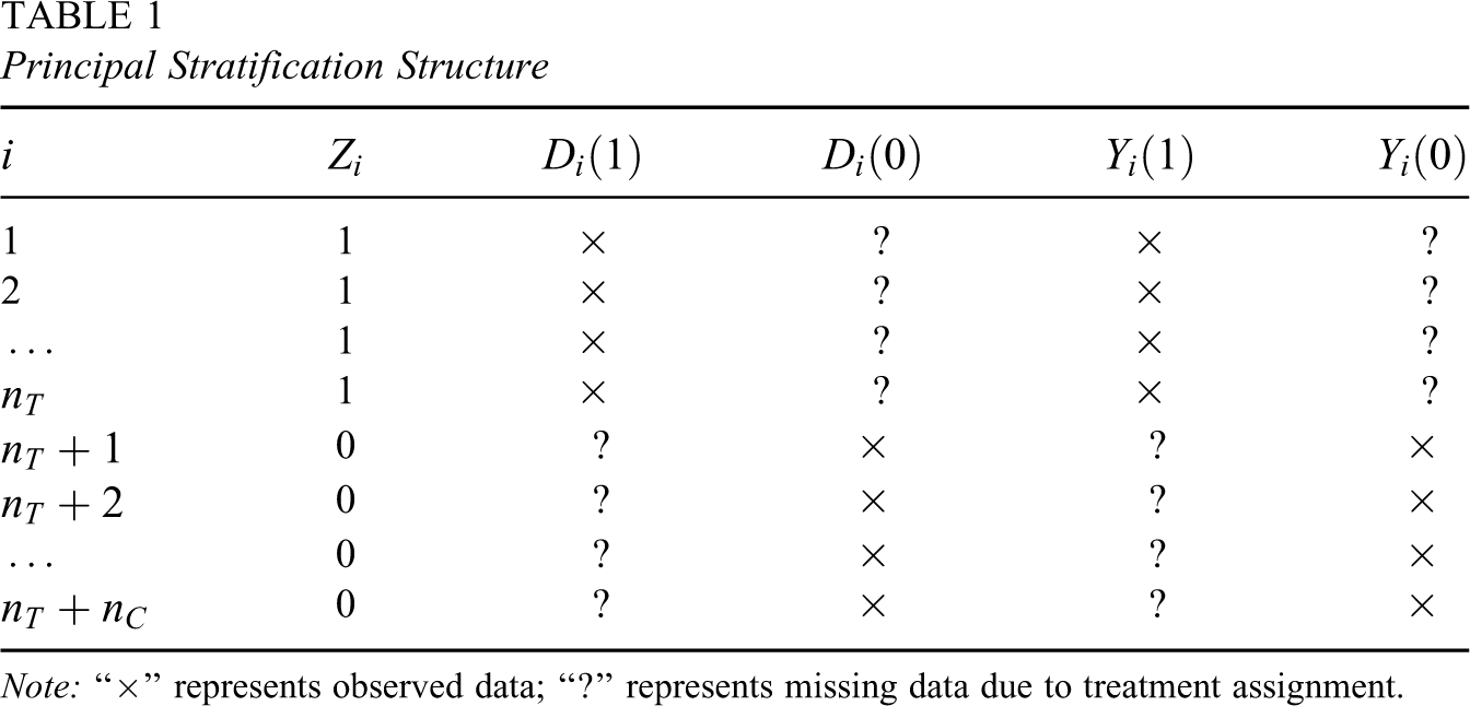
Suppose all the children have the same value of covariates for the moment, the principal stratification structure of the children is illustrated in Table 1, where the “×” represents observed data, and the “?” represents unobserved, or missing, data due to treatment assignment. If every child were a complier (i.e., if all the
Principal Stratification Structure
Principal Stratification Structure
Note: “
Now consider covariates. In this section, we assume the background covariates
With noncompliance, we can classify the children into four different principal strata: compliers, always-takers, never-takers, and defiers. Although the treatment assignment determines which component of the principal stratum
Here, we explain assumptions common in our approach and Barnard et al. (2003). Assumption 1: Stable Unit Treatment Value Assumption (SUTVA; Rubin, 1980). This assumption states that the treatment assignment of one child will not affect other children’s posttest scores and that there are no different versions of public schools that a particular child can attend, and analogously, there are no different versions of private schools. We consider this assumption reasonable, because the children in the experiment probably do not know each other, and they typically attend the closest private school or the closest public school from their home. The SUTVA is widely assumed in randomized experiments, and the representation of potential outcomes in Table 1 would not be adequate without it. Assumption 2: Ignorable Treatment Assignment (Rubin, 1978). Formally, Assumption 3: Monotonicity: Assumption 4: Exclusion Restriction: If
With the above four assumptions, there only exist three principal strata of children in the program: compliers, never-takers, and always-takers; and we are focused on the CACE, because the other two principal causal effects are assumed to be zero.
Missing Data
Missing Covariate and Outcome Data
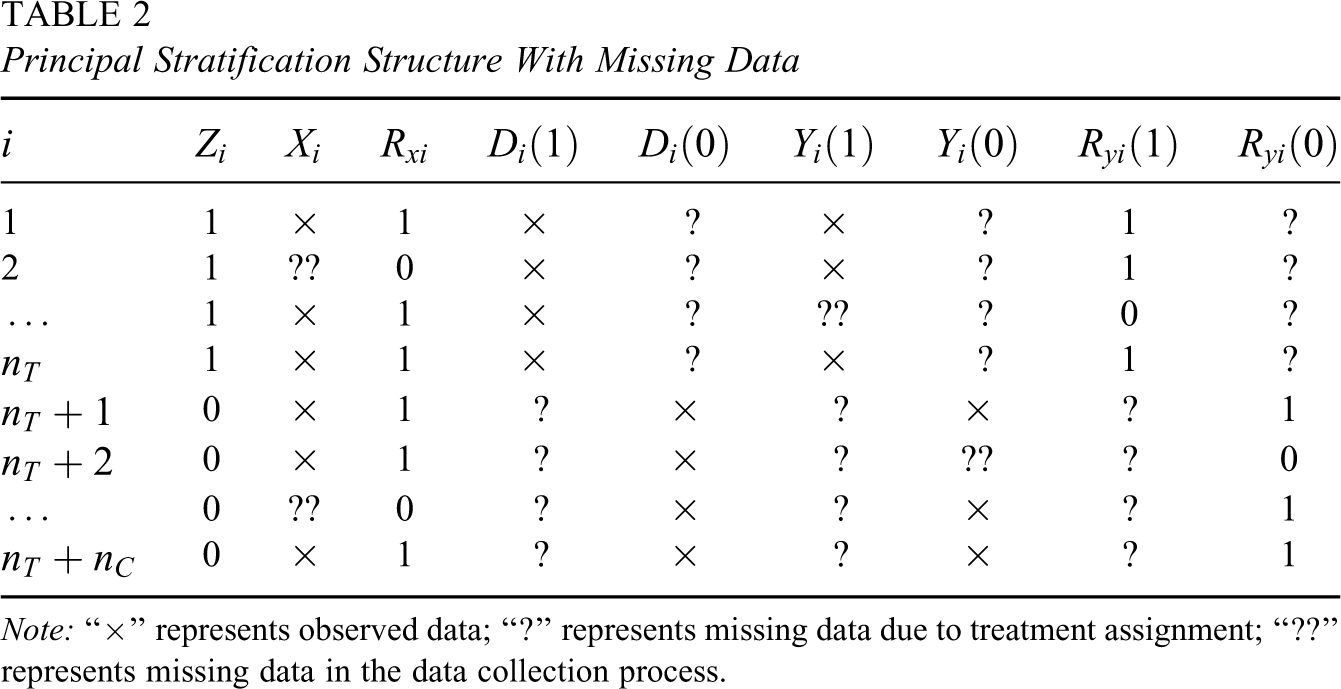
In the New York City School Choice Scholarship Program, some background covariates and outcomes could not be collected, which are depicted by “??” in Table 2. Note that these data should have been observed but were somehow missing in the data collection process of the experiment, thus different from the missing data due to treatment assignment depicted by “?” in the same table. We use an indicator vector
Principal Stratification Structure With Missing Data
Principal Stratification Structure With Missing Data
Note: “
We now consider possible assumptions with such a missing data problem, some of which also were explicitly made by Barnard et al. (2003). Assumption 5: Compound Exclusion Restriction. If Assumption 6: Ignorable Covariate Missingness. Assumption 7: Latently Ignorable Outcome Missingness.
Assumptions 1 through 7 lay the foundation for our analysis regardless of specific parametric models. In contrast, Barnard et al. (2003) assumed assumptions 1 through 5 and assumption 7 in a different form. Based on these assumptions, we can propose the modified general location model in the next section.
Modified General Location Model
Standard General Location Model
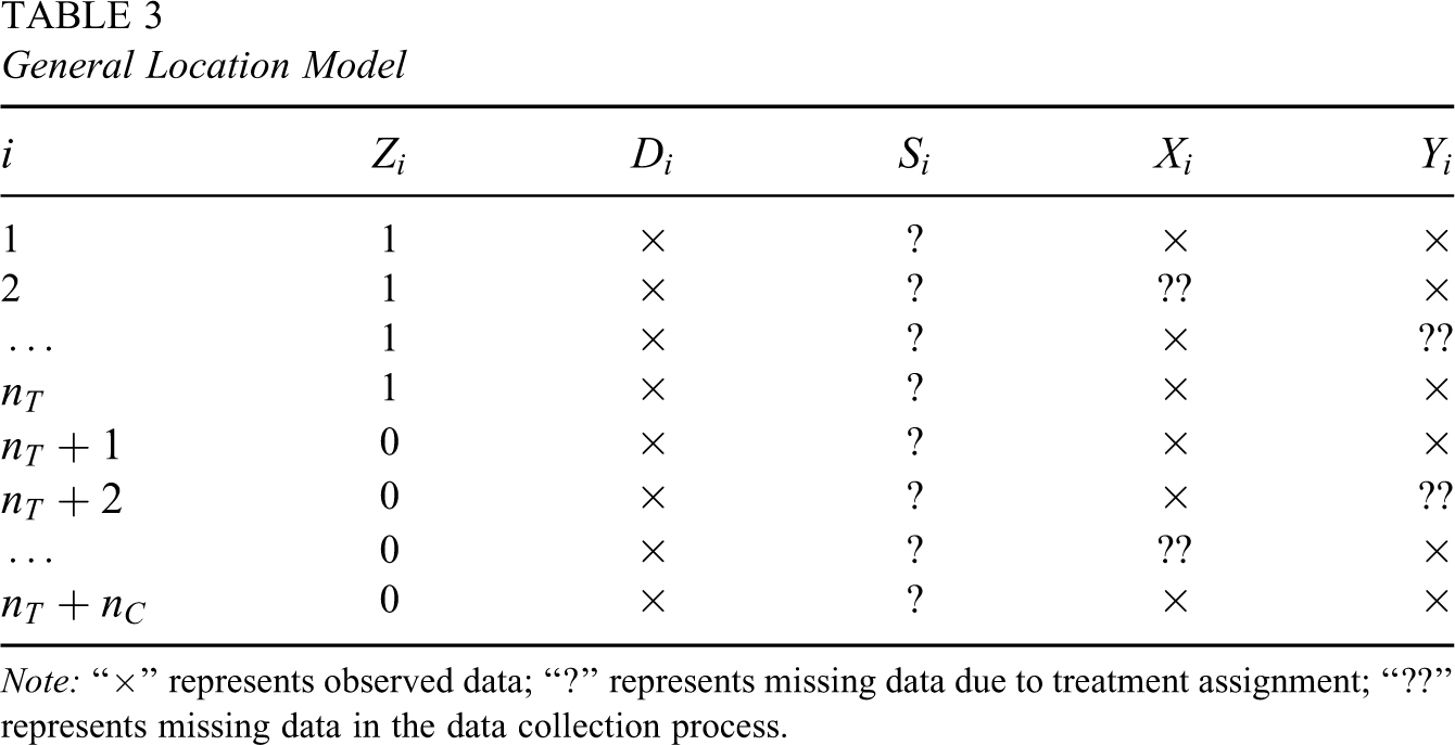
Table 2 can be transformed into Table 3 to illustrate the data structure we face from the computational perspective. There are three categorical variables: the binary treatment assignment
General Location Model
General Location Model
Note: “
If there were no restrictions imposed by our explicit assumptions discussed in Sections 3 and 4, a standard general location model (Schafer, 1997) could be used to compute the missing data in Table 3 and make inferences for the underlying parameters. This model assumes a multivariate normal distribution
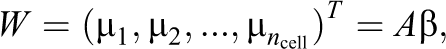
where the components of vector β are the unconstrained parameters. The categorical data follow a log-linear model:
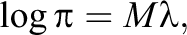
where π represents the probability vector for all the
Computational tools to make inferences for the parameters β,
Specifically, in the case of the standard general location model, we can apply ECM to obtain maximum likelihood (ML) estimates: Given the complete data, λ can be estimated using one cycle of iterative proportional fitting (IPF; Bishop, Fienberg, & Holland, 1975), and (β,
In Table 3, the value of
Contingency Table of General Location Model
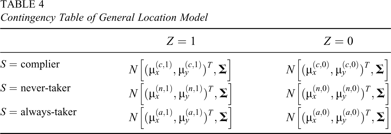
Contingency Table of General Location Model
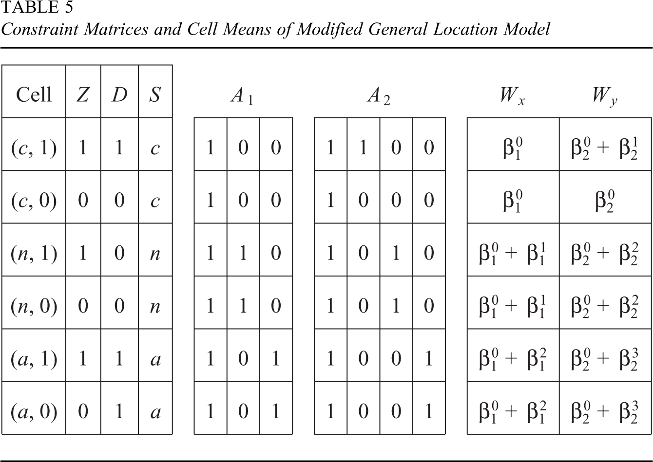
Now, we need to modify the standard general location model, by imposing two constraints to the cell means according to our explicit assumptions. Ignorable treatment assignment assumption. If the experiment is completely randomized, the continuous covariate variables in a treatment cell (Z = 1) should have the same distribution as those in the corresponding control cell (Z = 0). Specifically, the normal means for the continuous covariates X in the following cells should be the same:
In reality, there exist some design variables in the program, and so in our actual model in Section 5.3, the above relations hold within each “super” cell defined by those design variables, because all the other covariates are balanced in such cells of design variables by treatment assignment. Exclusion restriction assumption. Always-takers and never-takers should have zero causal effects. Therefore, the outcomes in a treatment cell should have the same distribution as the outcomes in the corresponding control cell. Specifically, the normal means for the outcomes Y in the following cells should be the same:

Note that
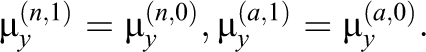
As a result of the above two constraints, we should modify the specification and computation of the standard general location model. First, we divide the continuous variables into two blocks, the covariate X block and the outcome Y block and impose different constraint matrices for their respective normal means:

More specifically, let the unconstrained parameters be
Constraint Matrices and Cell Means of Modified General Location Model
Second, we partition the common covariance matrix
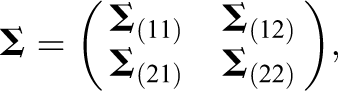
where
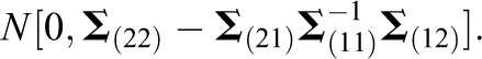
Third, we modify the computation for β1, β2, and

where the row of the random error
It is relatively straightforward to extend this two-block model into models with more blocks. Suppose we have L blocks of continuous variables, each of which has a specific constraint matrix

and the covariance matrix
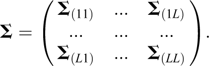
The extention in computation is also straightforward.
We actually use a four-block model for the single-child data in the program. The categorical variables are Z, D, S, application period (the PMPD period or not), applicant’s original school (low average score or high average score), and grades (1−4), which account for the design variables of the experiment.
We use the following four blocks of continuous variables: Block 1 includes two fully observed categorical background covariates (whether the child has received any foreign education, whether the father’s work status is missing) and two almost fully observed categorical covariates (sex, religion) and treats them as continuous variables (X
1); Block 2 includes two continuous background covariates (X
2): pretest reading score and pretest math score; Block 3 includes two continuous outcomes (Y): posttest reading score and posttest math score; Block 4 is the outcome missingness treated as a continuous variable (Ry
): whether the child takes the posttest.
In the above specification, we can treat the fully observed categorical data in Block 1 and Block 4 as continuous, because no missing data need to be estimated. For the two almost fully observed covariate variables in Block 1, we do not expect this approximation to significantly distort the results, because very few data (less than 5%) are missing. Of course, the more missing data in the categorical background covariates, the less appropriate it is to use this continuous approximation, and a better model to handle this issue is needed, as discussed in Section 7.
For the categorical variables in our modified general location model, we assumed a log-linear model that had two-way interactions of principal stratum S with application period, S with applicant’s original school and S with grade. We also imposed linear model constraints on the cell means that had main effects for S, application period, and grade along with all two-way interactions among these variables in addition to the constraints implied by ignorable treatment assignment and exclusion restriction.
Due to the latently ignorable outcome missingness assumption, the outcome missingness Ry
in Block 4 should be independent of the outcome values Y in Block 3, given the covariates X and the principal stratum S. Within each cell defined by the categorical variables, including S, we take
We applied our model to the 1,050 children in Grades 1 through 4 from single-child families, with a flat prior distribution for the parameters of our four-block Bayesian model. We first ran the EM algorithm to get the ML estimate of the parameters, and then used it as an initial value to run a Markov Chain Monte Carlo (MCMC) and draw the posterior samples of the parameters and the missing data. In each MCMC iteration, we simulated the parameters and the missing principal strata, missing covariates, and missing outcomes. After convergence, we obtained the posterior distribution of all estimands of interest: parameters, CACE, proportions of the three principal strata, and so on. To ensure convergence, we ran several separate chains starting from different initial values and applied the G-R statistic to monitor convergence (Gelman & Rubin, 1992).
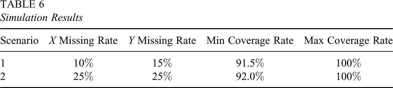
We developed our software using the S-PLUS code for the standard general location model provided by Schafer (1997), with corresponding modifications based on our discussion in this section. To check the validity of our software to and investigate the frequentist properties of our Bayesian model, we carried out a frequentist simulation as follows: We set the posterior median as the true underlying parameters; in each replication, we used the true parameters to generate a pseudo data set and made a certain proportion of the data missing completely at random (see Table 6 for the proportions); then we drew the posterior samples of the parameters using MCMC and examined whether each true scalar parameter was covered by its corresponding posterior 95% interval; we repeated such a replication 200 times, and we then obtained the coverage for each scalar parameter. We tried two different scenarios of the missingness: In the first scenario, we made 10% of the covariate data and 15% of the outcome data missing completely at random; in the second scenario, 25% of the covariate data and 25% of the outcome data were made missing completely at random. Table 6 displays the largest and the smallest coverage rates for those scalar parameters under the two scenarios. The simulation results show very good frequentist properties: The coverage rates are between 91.5% and 100%, which indicates that our software was written correctly. A more extensive Bayesian assessment would have used the method of Cook, Gelman, and Rubin (2006). In addition, the increase of missing data proportion does not appear to affect the coverage rates. To test the sensitivity of the results to different values of the true underlying parameters, we increased and then decreased certain individual components of the parameters by 20%, and there was little difference from the results in Table 6.
Simulation Results
Simulation Results
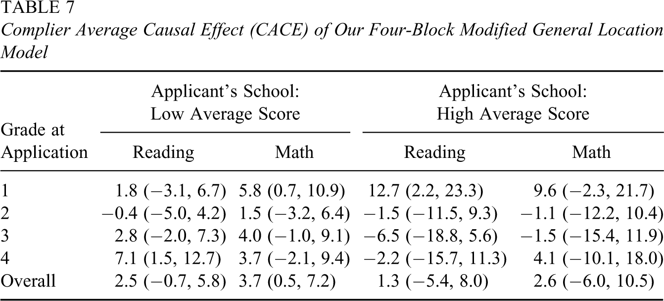
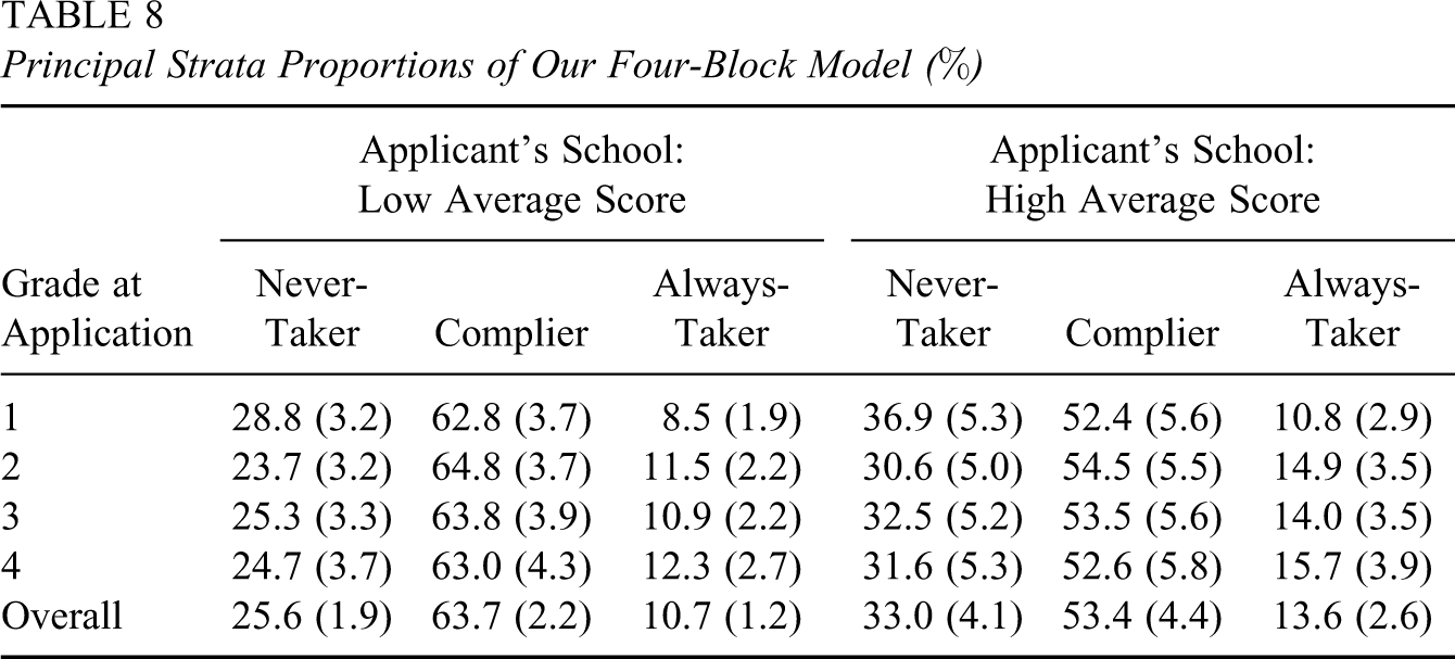
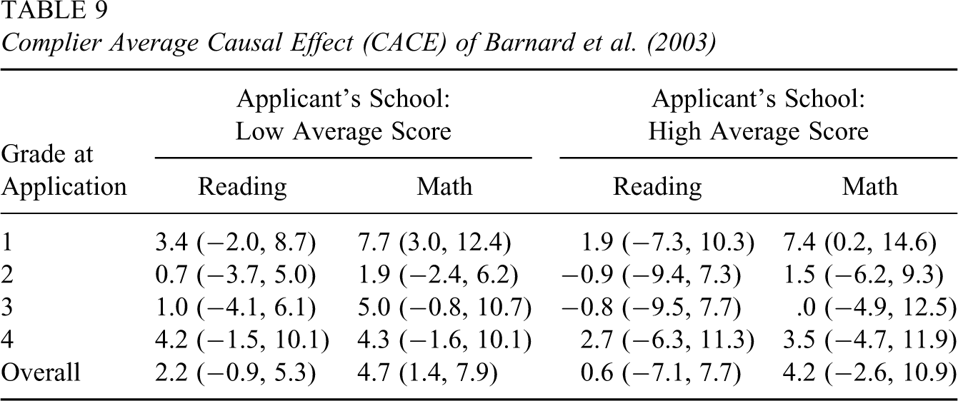
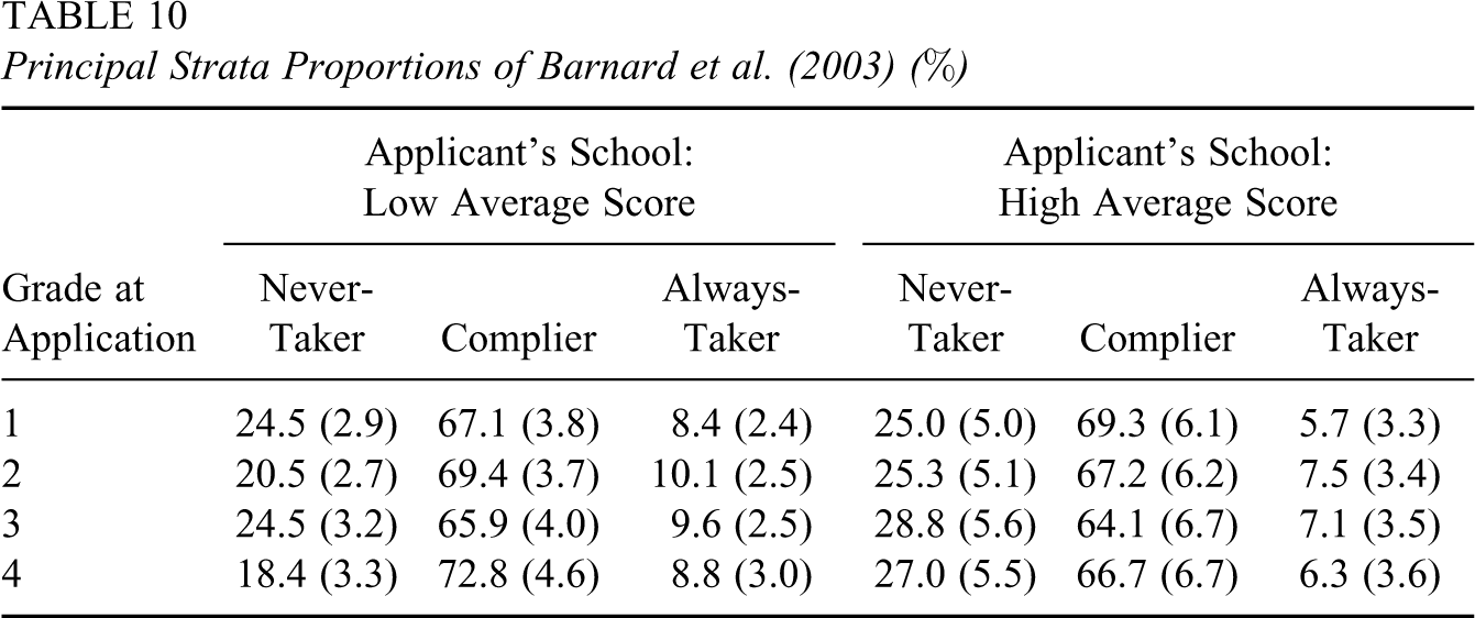
We summarize the posterior distribution of CACE, and principal strata proportions, within each group defined by the applicants’ grade at the time of application and whether their original public schools had an average test score higher or lower than the citywide median. Table 7 reports the posterior mean and posterior 95% interval of CACE for each group. Table 8 lists the posterior means and posterior standard deviations for the percentages of all three principal strata in each group. The corresponding results in Barnard et al. (2003) are shown in Tables 9 and 10, respectively.
Complier Average Causal Effect (CACE) of Our Four-Block Modified General Location Model
Complier Average Causal Effect (CACE) of Our Four-Block Modified General Location Model
Principal Strata Proportions of Our Four-Block Model (%)
Complier Average Causal Effect (CACE) of Barnard et al. (2003)
Principal Strata Proportions of Barnard et al. (2003) (%)
The results of CACE in Table 7 look very similar to those in Table 9: Most of the posterior means are positive but below 10, and most of the 95% intervals cover zero. However, both models find that for compliers originally from schools with low average scores, attendance in private school will unambiguously improve their overall math performance (3.7 [0.5, 7.2] in Table 7; 4.7 [1.4, 7.9] in Table 9) as compared to attendance in public school. Such an improvement is especially evident for children in Grade 1 (5.8[0.7, 10.9] in Table 7; 7.7 [3.0, 12.4] in Table 9). However, results from the two models differ in some other groups in Tables 7 and 9: Using our model, we find that reading score was likely improved for children from Grade 4 of low average schools (7.1 [1.5, 12.7]) and children from Grade 1 of high average schools (12.7 [2.2, 23.3]); the estimates of Barnard et al. (2003) of the two groups, 4.2 (−1.5, 10.1) and 1.9 (−7.3, 10.3), respectively, were much smaller. They instead found that complying children from Grade 1 of high average schools likely enjoyed an increase in math score (7.4 [0.2,14.6]) by attending private school, in contrast to 9.6 (−2.3, 21.7). Their results are consistent in contrast with our higher but more uncertain estimates.
As shown in Table 8, our model found a posterior distribution of principal strata proportions similar to that in Table 10: Compliers account for a majority of the children, and always-takers turn out to be the smallest principal stratum. This is understandable, because all the children are supposed to come from poor families and can not attend private school without the scholarship. However, our model tends to predict a somewhat smaller size of the complier stratum and slightly larger sizes of the other two strata than Barnard et al. (2003), especially for children from high average score public schools.
Although our modified general location model and the model in Barnard et al. (2003) differ in some underlying assumptions, selection of covariates, and the actual parametric form, we share the same principal stratification framework. This might be one explanation for the similar result of the math improvement of complying children from low average score schools, which is different from the result in Peterson et al. (1999). Another similar result of Barnard et al. (2003) and ours is the proportional distribution of principal strata, which also provides interesting evidence for policymaking.
The relatively minor differences in the results from the two analyses, such as the reading improvements for certain groups, are possibly partly due to the missing covariate values that we make use of in our model, although more detailed examination is needed for such a conclusion. In general, our model seems to be a useful alternative to theirs, because we can use the information contained in those missing covariates otherwise ignored.
However, we have also made some simplifications for computational convenience, such as treating some categorical variables as continuous. This is generally fine for our current model, because the four categorical covariates we used in Block 1 are either fully observed or almost fully observed, and the outcome missingness Ry in Block 4 is also fully observed. However, our current model might encounter some difficulties if the outcome variable itself is categorical and partially observed. Therefore, such a specification calls for improvements in our future work, which hopefully should include all the categorical variables, whether covariate or outcome, in the categorical part of the general location model. In that case, the log-linear model for the categorical part may require further modifications.
Footnotes
Acknowledgments
This work was supported in part by NFS Grant SES-05-05887 and NIH Grant R01 DA023879-01.