
Abstract
When fitting hierarchical regression models, maximum likelihood (ML) estimation has computational (and, for some users, philosophical) advantages compared to full Bayesian inference, but when the number of groups is small, estimates of the covariance matrix (Σ) of group-level varying coefficients are often degenerate. One can do better, even from a purely point estimation perspective, by using a prior distribution or penalty function. In this article, we use Bayes modal estimation to obtain positive definite covariance matrix estimates. We recommend a class of Wishart (not inverse-Wishart) priors for Σ with a default choice of hyperparameters, that is, the degrees of freedom are set equal to the number of varying coefficients plus 2, and the scale matrix is the identity matrix multiplied by a value that is large relative to the scale of the problem. This prior is equivalent to independent gamma priors for the eigenvalues of Σ with shape parameter 1.5 and rate parameter close to 0. It is also equivalent to independent gamma priors for the variances with the same hyperparameters multiplied by a function of the correlation coefficients. With this default prior, the posterior mode for Σ is always strictly positive definite. Furthermore, the resulting uncertainty for the fixed coefficients is less underestimated than under classical ML or restricted maximum likelihood estimation. We also suggest an extension of our method that can be used when stronger prior information is available for some of the variances or correlations.
Keywords
Hierarchical or mixed-effects regression models are increasingly popular in applied statistics and can be viewed as Bayesian at the following two levels: A prior distribution is assigned to the varying coefficients, and the parameters of that prior distribution themselves are given a hyperprior. The family of models can be written in general terms as follows: Data are in groups j = 1,… J. For each group j, there is a response vector
There is a rich literature on full Bayesian inference for hierarchical regressions. There is also an empirical Bayes version in which the hyperparameters (in this case, Σ) are estimated via maximum likelihood (ML) and then inference for the coefficients is performed conditional on the estimated Σ. From the Bayesian perspective, the empirical Bayes approach is suboptimal, both because it avoids the use of any prior information on Σ and because it understates posterior uncertainty. From a pragmatic perspective, however, we recognize that the point estimation approach has two advantages that give it great appeal to many users. First, existing software such as lme4 in R and various commands in Stata allow such models to be fit fast and reliably for moderate-sized data sets, whereas software for Markov chain Monte Carlo simulation for full Bayes inference is not yet so immediately practical. Second, the non-Bayesian motivation behind point estimation is attractive to practitioners who want the benefits of partial pooling and hierarchical modeling without needing to specify prior information or fully buy into the Bayesian paradigm.
The subject of this article is the use of Bayesian ideas and methods to produce better inferences for hierarchical models via better point estimates of the hyperparameters. In that sense, this work falls into a long tradition of Bayesian tools used for practical non-Bayesian inferences (e.g., Agresti & Coull, 1998). Bayes modal (BM) estimation (or penalized likelihood) has also been used to obtain more stable estimates in item response theory (e.g., Mislevy, 1986; Swaminathan & Gifford, 1985; Tsutakawa & Lin, 1986) and to avoid boundary estimates (or logit parameters tending to ±∞) in log-linear models (Galindo-Garre, Vermunt, & Bergsma, 2004), logistic regression (Gelman, Jakulin, Pittau, & Su, 2008), varying-intercept models with constant coefficients (Chung, Rabe-Hesketh, Dorie, Gelman, & Liu, 2013), random-effects meta-analysis models (Chung, Rabe-Hesketh, & Choi, 2013), and latent class analysis (Galindo-Garre & Vermunt, 2006; Maris, 1999). Such an approach has also been used to obtain nondegenerate covariance matrices in factor analysis (Martin & McDonald, 1975), in finite mixtures of normal densities (Ciuperca, Ridolfi, & Idier, 2003; Vermunt & Magidson, 2005), and in multivariate regression (Warton, 2008). In varying intercept models, the Stein loss function (Srivastava & Kubokawa, 1999) and an extension of MANOVA estimation (Amemiya, 1985) have been used for obtaining nonnegative definite covariance estimators.
The key problem solved by our method is the tendency of ML estimates of Σ to be degenerate, that is, on the border of positive definiteness, which corresponds to zero variance or perfect correlation among some linear combinations of the parameters. When the ML estimate of a hierarchical covariance matrix is degenerate, this often arises from a likelihood that is nearly flat in the relevant dimension and just happens to have a maximum at the boundary.
Our solution is a class of weakly informative prior densities for Σ that go to zero on the boundary as Σ becomes degenerate, thus ensuring that the posterior mode (i.e., the maximum penalized likelihood estimate) is always nondegenerate. We recommend a class of Wishart priors with a default choice of hyperparameters, that is, the degrees of freedom is the dimension of
In a simulation study and an education example presented later, the default Wishart prior always gives nondegenerate estimates of Σ (in particular, nonperfect correlation coefficients) without decreasing the log likelihood substantially. The BM estimators of the standard deviations and correlations using the default Wishart prior have better statistical properties than the (restricted) ML estimators.
When prior information is available for specific standard deviations or correlations, additional penalty functions may be included. Specifically, if the prior most plausible value for a standard deviation or correlation parameter is σ* or ρ*, respectively, then we propose multiplying the Wishart prior by the gamma(2, 2/σ*) or N(ρ*, .252) densities. This assigns more prior probability around the preferred values while exploiting the property of the Wishart prior that it ensures that the estimates remain positive definite.
The outline of the article is as follows. First, we illustrate the boundary estimation problems encountered in ML estimation of hierarchical variance and covariance parameters. Then, we introduce the default Wishart prior for Σ and investigate its properties. Next, additional penalty functions are proposed that incorporate further prior knowledge for some of the parameters. Finally, our method is applied to an example from education research and simulated data.
Boundary Estimation Problem
Consider the varying-coefficients model,

where yij
is the response variable for unit i in group j,
Non-Bayesian Point Estimation
For each j,

where the constant term, −(N/2)log(2π), has been dropped. The ML estimator is obtained by maximizing the log-likelihood function.
It is known that the ML estimator of the covariance matrix is biased for finite samples (Lehmann & Casella, 1998), and an often-preferred option is restricted maximum likelihood (REML; Patterson & Thompson, 1971), as it takes into account the degrees of freedom for the fixed coefficients
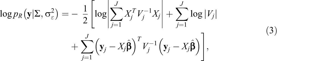
up to a constant, where

Singular Estimates of Σ using ML and REML
ML and REML often yield singular (i.e., nonpositive definite) estimates of Σ. This boundary includes the cases where some varying coefficients have zero variance or a varying coefficient is a linear combination of the other varying coefficients.
We present two simulation studies to demonstrate how often singular estimates of Σ occur in the varying-coefficients model. In the first study, we consider a model with two-dimensional varying coefficients, that is, a varying intercept b
0j
and a varying slope b
1j
. We set the group size to n = 10 and the number of groups to J = 5 or 10. A covariate that varies within group only was generated from N(0, 1) and group-mean centered. The varying coefficients (b
0j
, b
1j
) were generated from N(
Figure 1a shows the proportion of ML estimates of Σ on the boundary for the two-dimensional case. For J = 5 groups, 87% of the ML estimates are singular when σ = 0.25 and the proportion decreases as σ increases but remains as high as 72% when σ = 1. For J = 10 groups, the proportions are smaller than those for J = 5 but still, in more than 40% of the simulations, the likelihood is maximized at a singular
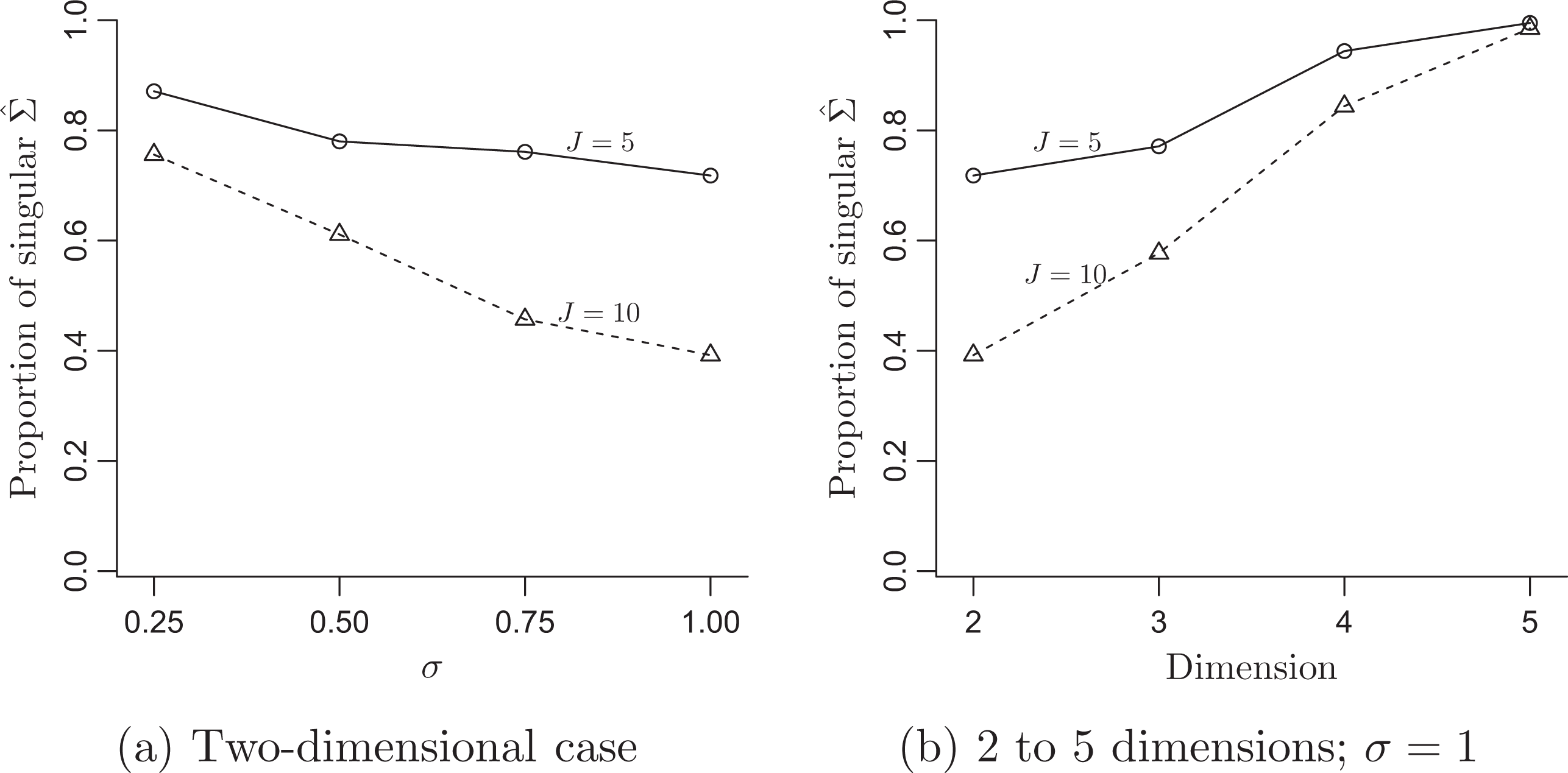
Proportion of data sets, out of 1,000, where the maximum likelihood (ML) estimate of the covariance matrix is singular. (a) Two-dimensional case: When σ = .25, 87% of the ML estimates are singular for J = 5. As σ and J increase, the proportion decreases but is greater than 40% for the conditions considered. (b) Two to five dimensions σ = 1: As the dimension of Σ increases, there is a rapid increase in the probability of the estimate being degenerate.
Our second simulation study considers various dimensions, from d = 2 to d = 5, each time with a varying intercept and d − 1 varying slopes for n = 10 and J = 5 or 10. The d − 1 covariates were independently drawn from N(0, 1) and centered at their group means as in the previous simulation. The varying coefficients
In some contexts, singular estimates of the covariance matrix are acceptable or considered as an indication of structural misspecification of the model. In the varying-intercept model, a negative group-level variance estimate is sometimes permitted if the model is viewed as a marginal model for the responses, given the covariates where only the sum of the group-level and within-group variance must be positive (Verbeke & Molenberghs, 2000, pp. 52–53). In factor analysis and structural equation models, a negative variance estimate, called a Heywood case, is sometimes interpreted as model misspecification, especially if the null hypothesis that the variance is nonnegative can be rejected (Kolenikov & Bollen, 2012). However, this article takes a hierarchical perspective of the multilevel linear model, where the intercepts and slopes vary due to omitted group-level variables. Therefore, the variances of the varying coefficients must be nonnegative, and perfect correlations among linear combinations of varying coefficients are regarded as unrealistic.
Weakly Informative Wishart Prior for Σ
We propose posterior modal estimation with a prior on Σ, implicitly assuming uniform priors for the other parameters. With a prior p(Σ), the log-posterior function can be written as follows:

and we find the mode of

where
If we set Ψ to be a diagonal matrix (1/2θ)Id , the Wishart density of Σ in Equation 5 can be written as:


where λ1,…, λ
d
are the eigenvalues of Σ and
As a default choice, we propose
The advantage of this family of density functions is that they equal zero at the boundary—thus, the BM or penalized likelihood estimate for Σ will never be degenerate—but the densities move away from zero when Σ moves off the boundary, so that the posterior mode can be arbitrarily close to degeneracy if this is what the data demand. In contrast, various other families of models do not have these properties, making them less desirable when used for the purpose of BM point estimation. The inverse-Wishart family of density, one of the most commonly used priors for Σ in the full Bayesian inference, is also zero at the boundary. However, it tends to assign an excessive penalty near the boundary because it is a function of Σ−1 and
Alternative choices of
Priors on the covariance matrix in the varying-coefficients model have been investigated by several authors in the context of full Bayesian modeling. Daniels and Kass (1999) investigated nonconjugate Bayesian estimation of covariance matrices in hierarchical models including an inverse-Wishart prior on covariance matrices with unknown scale and degrees of freedom and a normal prior on Fisher’s z-transformed correlations. Barnard, McCulloch and Meng (2000) decomposed
Unlike posterior mean estimation, BM estimation does not involve simulation and is computationally as efficient as ML estimation. By modifying existing ML estimation procedures, gllamm (Rabe-Hesketh, Skrondal, & Pickles, 2005) in Stata and lmer (Bates & Maechler, 2010) in R, we have developed software to find the maximum of the penalized likelihood. The modified gllamm is available from www.gllamm.org and blmer, the modified lmer function, can be found in the blme package available from the Comprehensive R Archive Network.
Varying-Intercept Models: d = 1
The varying-intercept model is a special case of the model in Equation 1 with d = 1, given by:

where
When θ → 0, the gamma(1.5, θ) prior on
In the context of small area estimation, strictly positive group-level variance estimators have been proposed for the Fay and Herriot model (1979), a varying-intercept model for aggregated group-level data and known heterogeneous within-group variances. Adjustment for density maximization (Li & Lahiri, 2010; Morris, 2006; Morris & Tang, 2011) applies a penalty term
Varying-Intercept and Varying-Slope Models: d = 2
When d = 2, the model includes a varying intercept and a varying slope of one covariate, written as:

where
As shown in Equation 6, with the default choice ν = d + 2, the Wishart density can be written as a product of gamma(1.5, θ) densities on the eigenvalues λ1 and λ2. For the bivariate case, we can also express the default prior as a function of the variances (

This expression implies that Wishart(4, (1/2θ)Id
) with θ → 0 is equivalent to the joint density of independent gamma(1.5, θ) priors on both
Since the beta(1.5, 1.5) prior on (ρ + 1)/2 is zero at the boundaries ρ = ±1, the posterior mode of Σ cannot be attained at any matrices with perfect correlation. In addition, the beta(1.5, 1.5) density function increases rapidly as ρ approaches 0 from ±1 and so does not rule out values close to ±1. The left panel of Figure 2 shows the beta(1.5, 1.5) density on (ρ + 1)/2. Whereas gamma(2, θ) increases linearly at 0, the slopes of beta(1.5, 1.5) at ±1 are ±∞. Therefore, compared to the gamma(2, θ) prior for σ1 and σ2, the beta(1.5, 1.5) for ρ is less informative with lower penalties on the values around the boundaries.
Conditional density of ρ
ij
with Wishart (d + 2, (1/2θ)I) on
The beta priors have been used to avoid boundary estimates of the probability parameter p of the binomial distribution. When the sample proportion is 0 or 1, the traditional Wald confidence interval for p degenerates to the point estimate. To avoid such boundary estimates, Agresti and Coull (1998) specified a beta(2, 2) prior on p. The posterior mean of p then is the sample proportion after adding two successes and two failures to the data. Compared with the beta(2, 2), the beta(1.5, 1.5) tends to assign less penalty at the boundaries and so is less informative.
Higher Dimensional Case: d ≥ 3
Similar to the case d = 2, the default prior for d ≥ 3 can be written as a product of σ r , r = 1,…, d and a function of ρ rs , the correlation between the rth and sth varying effects (0 < r < s, s = 2,…, d). For example with d = 3, the Wishart(5, (1/2θ)I 3) prior with θ → 0 can be written as:

This is a product of gamma(1.5, θ) priors on the variances and a function of the correlations. This function depends on the squares of the correlations, as in the two-dimensional case (Equation 7), but also contains the product of three correlations, which comes from the constraint
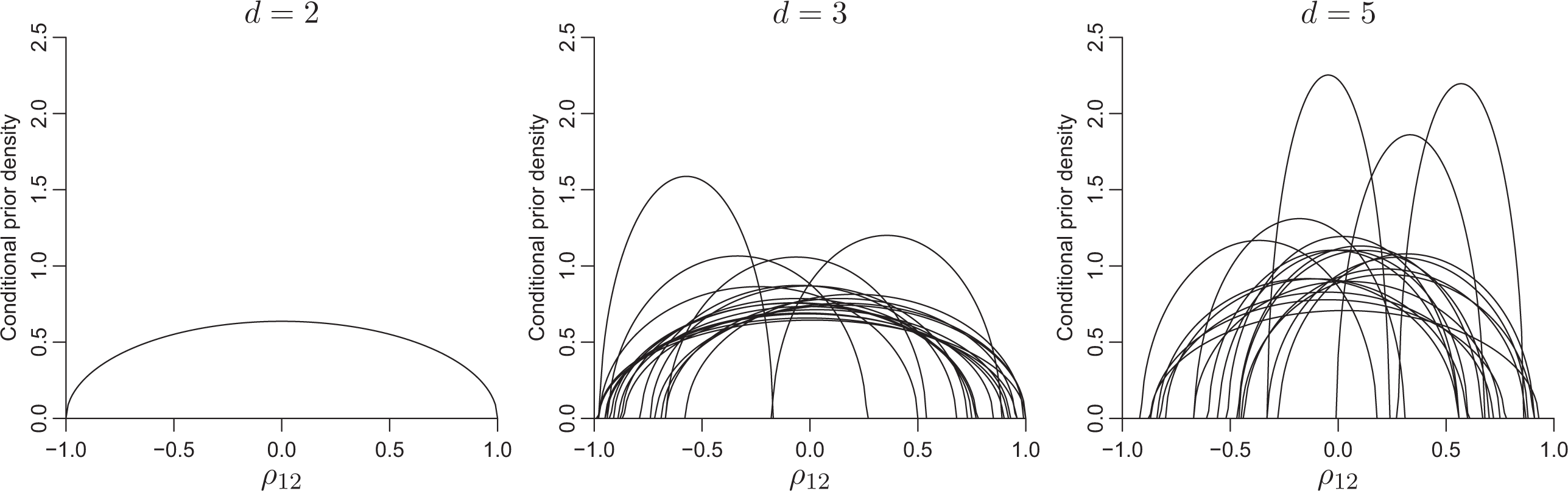
The graphs in Figure 2 show the conditional densities of ρ12 when Σ follows the Wishart(d + 2,(1/2θ)Id
), θ = 10−4. The curves are the density of ρ12 conditional on the other parameter values (standard deviations and the other correlations) that are randomly generated from Wishart(d + 2,(1/2θ)Id
) with 20 replicates. When d = 2, the correlation follows beta(1.5, 1.5) as discussed previously. When d = 3, the curves have distinct supports, defined by
The marginal prior densities of ρ rs are displayed in Figure 3 for d = 2, 5, and 10. With 10,000 replicates, d-dimensional matrices were randomly generated from the Wishart(d + 2,(1/2θ)I) with θ = 10−4 and 10,000(d − 1)(d − 2)/2 correlation coefficients were used to construct the histograms. For d = 2 (left), the distribution of the correlation coefficient matches the beta(1.5, 1.5) density, shown as a solid curve. As d increases, the marginal prior density of ρ rs becomes more concentrated around zero because of the positive definiteness of Σ.
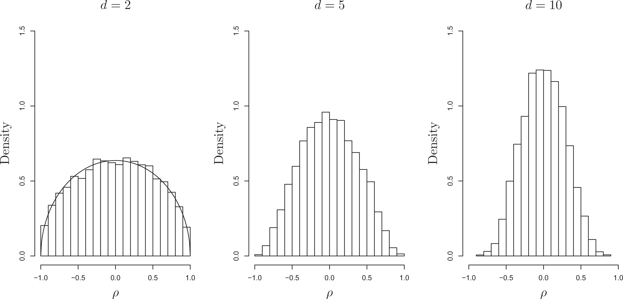
Marginal density of ρ rs with Wishart (d + 2,(1/2θ)I), θ = 10−4. When d = 2, the marginal density of ρ is equivalent to beta(1.5, 1.5) on (ρ + 1)/2 (solid curve). As d increases, the marginal density has more mass around 0 due to the positive semidefinite constraint of the covariance matrix.
Incorporating Additional Prior Information
In the previous section, we suggested the Wishart(d + 2,(1/2θ)I) with θ → 0 as a default prior when no other information is available. If a researcher has additional prior knowledge about any specific standard deviations or correlations, he or she might want to adjust the prior to incorporate such information. In this section, we suggest multiplying the Wishart prior by functions of the parameters on which we have information. Because the Wishart density ensures that Σ is positive definite, we can choose the functions for the other parameters to be intuitive and easy to specify without regard for the parameter space.
If σ* is a plausible value for σ
r
, then the gamma(2,2/σ*) density is recommended as a penalty. Recall that the default Wishart prior is proportional to gamma(2,θ) priors with θ → 0 on each standard deviation, multiplied by a function of the correlations. When the gamma(2,2/σ*) density of σ is multiplied by the Wishart, the part including σ
r
becomes
If any specific correlation ρ rs is believed to be close to ρ*, we can incorporate this prior information by multiplying the default Wishart prior by a N(ρ*,τ2) density. As usual, the scale parameter τ can be chosen depending on the prior uncertainty regarding ρ rs . A possible default choice is τ = .25 because it is the standard deviation of the beta(1.5,1.5) distribution. Figure 4 displays the shape of conditional prior densities of ρ12 with additional normal priors in the three-dimensional case. When ρ13 and ρ23 are fixed at zero (left), the default Wishart(5,(1/2θ)I 3) prior (solid curve) is pretty flat. In order to incorporate the prior information, for example, ρ* = −.5, the Wishart is multiplied by the N(−.5, .252) density, and then the prior mode moves toward −.5 (dashed curve). When ρ13 and ρ23 are .5 (middle and right), the support of the Wishart for ρ12 is on [−0.5, 1] because of the constraint of positive definiteness. When our prior value is on the boundary ρ* = −.5 (middle), the Wishart multiplied by N(−.5, .252) density is skewed toward −.5, but still enforces positive definiteness. When the prior value is inside the support, ρ* = −.5, the resulting density is less skewed (right).
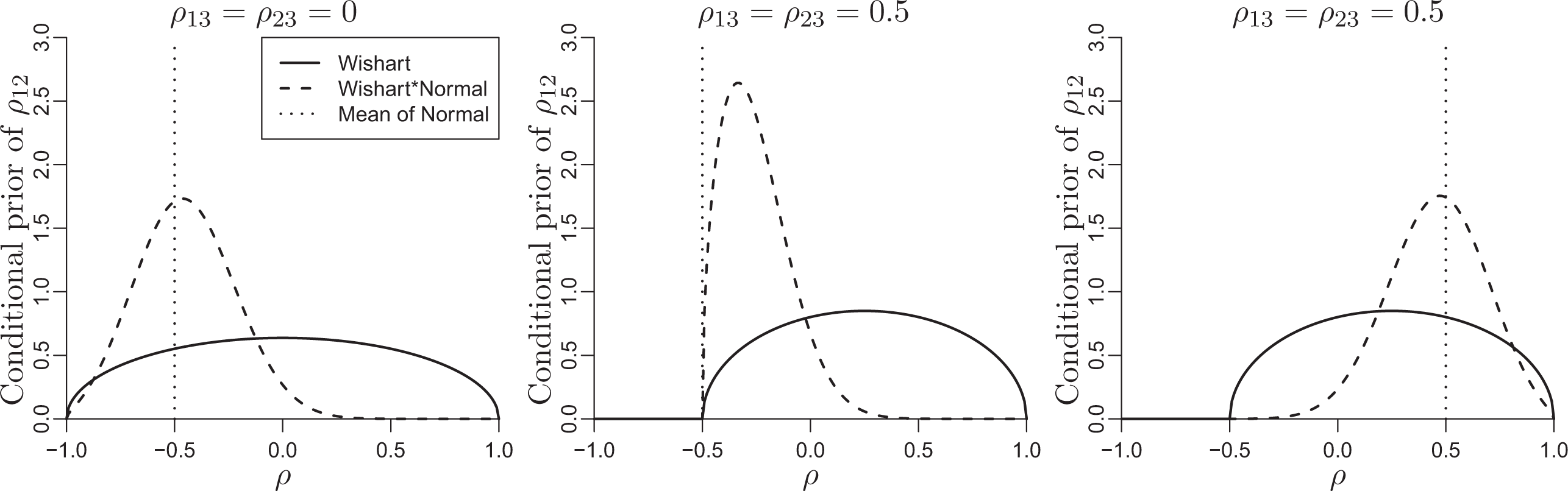
Conditional prior density of ρ12 with additional N(−.5, .252) (left and middle) and N(.5, .252) (right) densities multiplying the default Wishart prior. The Wishart prior is on three-dimensional
The default prior for ρ in the two-dimensional case is beta(1.5, 1.5), and so it would seem natural to use the beta family for ρ
rs
when constructing an additional penalty. However, the parameters of the normal distribution are more intuitive because they represent the prior mean (and mode) and variance. In addition, since the positive definiteness of
Example: A Varying Intercept, Varying Slope Model in Education Research
We illustrate our approach using a study of Heller et al. (2007) on the effects of the Mathematics Pathways and Pitfalls (MPP) teacher professional development program on mathematics learning for students at different levels of English language proficiency. Half of the 36 teachers were randomized to MPP and the other half to the control condition. Teachers randomized to the MPP condition were taught how to use the materials and then substituted MPP for part of their mathematics curriculum during the 2003–2004 school year, while control teachers used their regular mathematics curriculum. All students received an MPP test as a pretest before the lessons and took the same test after the lessons as a posttest.
Posttest scores are regressed on the mean-centered pretest scores, an indicator for treatment group (1 for MPP and 0 for control), English language learner (ELL) status (1 for ELL and 0 for non-ELL), and the Treatment × ELL Interaction Term. A varying intercept and a varying slope for ELL status are included to allow for the cluster-randomized design. The model can be written as follows:

where yij
is the posttest score for the ith student of the jth teacher,
Table 1 presents ML, REML, and BM estimates with the default Wishart(4,(1/2θ)Id ) prior with θ = 10−4. Both ML and REML estimates of the correlation between b 0i and b 1j are −1. This implies an unrealistic perfect correlation between the teacher-level slopes and intercepts. The BM estimate of ρ is −.32 and the standard deviation estimate of the varying slope for ELL status increases from 0.71 for ML and 0.48 for REML to 3.64, a change that is within the uncertainty implied by the asymptotic standard error of 2.1 (ML) or 2.2 (REML) for that parameter. The standard deviation of the varying intercept stays similar for ML, REML, and BM.
Parameter estimates for education example
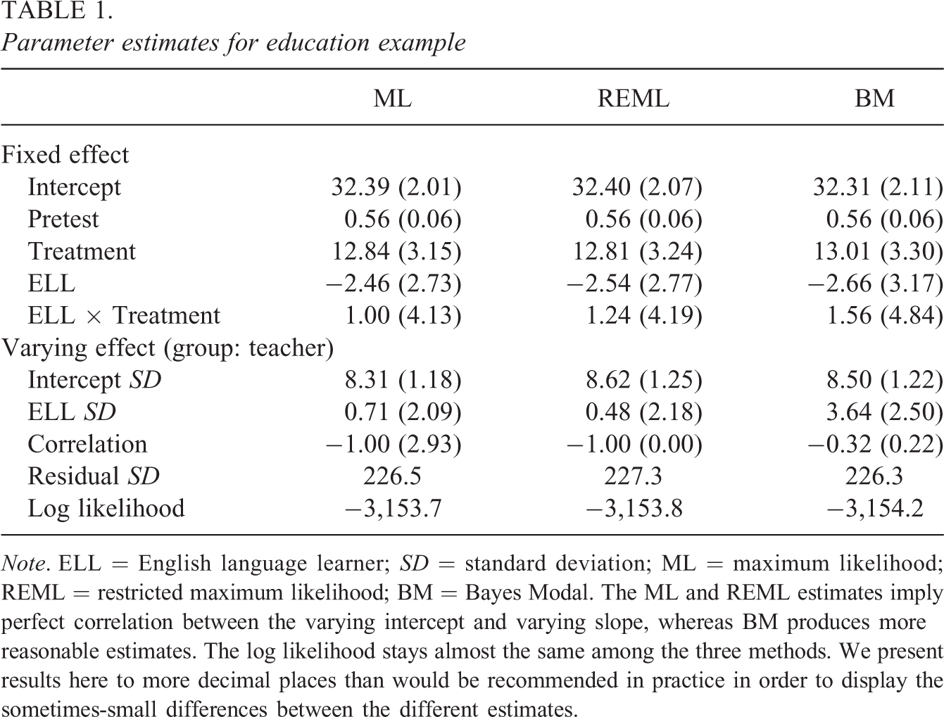
Note. ELL = English language learner; SD = standard deviation; ML = maximum likelihood; REML = restricted maximum likelihood; BM = Bayes Modal. The ML and REML estimates imply perfect correlation between the varying intercept and varying slope, whereas BM produces more reasonable estimates. The log likelihood stays almost the same among the three methods. We present results here to more decimal places than would be recommended in practice in order to display the sometimes-small differences between the different estimates.
The fixed coefficient estimates are similar across estimation methods. The coefficient for the interaction term between ELL and treatment changes the most among all the fixed coefficients, but the differences are negligible considering that the standard errors of the interaction term are greater than 4. The standard errors of the fixed coefficient estimates of Treatment, ELL, and Treatment by ELL are larger for BM than for ML or REML, suggesting that ML and REML underestimate the uncertainty.
The log likelihood at the BM estimates differs from the maximum by less than 1. Figure 5 shows the profile likelihood of ρ (profiling out all the other parameters) divided by its maximum. Although the ML is attained at ρ = −1, the profile likelihood is very flat and so the minimum (at ρ = 1) is attained with only an 8% decrement from the maximum. Therefore, all the values of ρ including ρ = −0.32 are well supported by the data. As is typical in such settings, there is nothing special about the point estimate on the boundary, and it would be inappropriate for a researcher to use that estimate. Our BM approach gives a default procedure that allows a classical statistician to avoid the inappropriate degenerate estimate. A full Bayes approach using real prior information would do better, but our BM approach takes us a bit in the right direction and has the advantage of being fast and easy to implement.
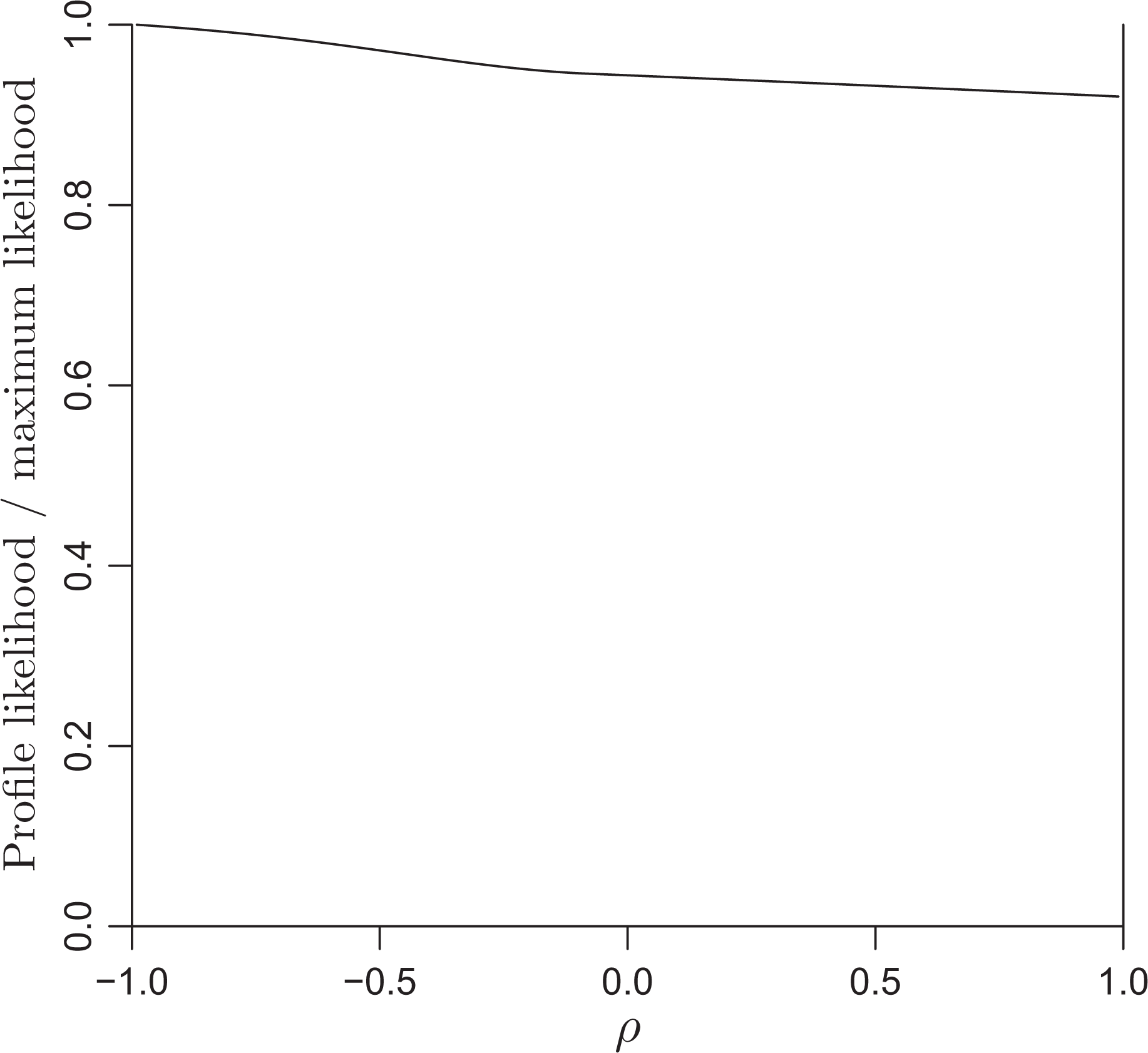
Profile likelihood of ρ. The maximum likelihood estimate of ρ is −1 but the likelihood has very little information. Therefore, the Bayes modal estimate of −0.3 is also well supported by the data.
When a researcher is interested in comparing teacher-specific effects, b 0j and b 1j can be predicted by their conditional posterior means (or modes), given the estimates of the model parameters and the data (called empirical Bayes prediction or best linear unbiased prediction).
In Figure 6, scatter plots of empirical Bayes predictions of b
1j
versus b
0j
are displayed with the proportion of ELL students of each teacher represented by the gray scale, that is, black indicates all the students are ELL and white indicates none are ELL. The sizes of the squares are proportional to the numbers of students for each teacher. For ML (left), due to the estimate
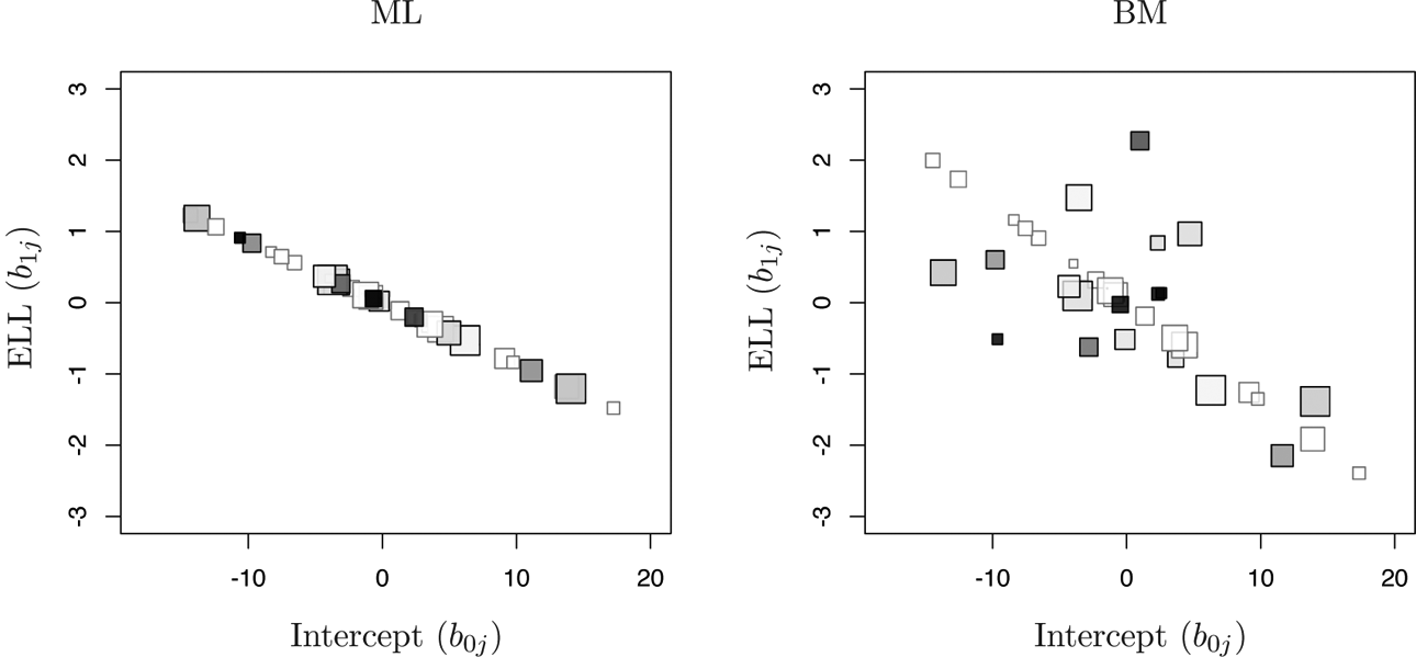
Empirical Bayes predictions of varying effects. The size of each square represents nj for the jth teacher. The ratio of English language learner (ELL) students for each teacher is shown on a gray scale, that is, black indicates all the students are ELL and white indicates none are ELL. For maximum likelihood, b 1j are predicted perfectly linearly in b 0j . On the right graph, Bayes modal estimation shows more reasonable predictions for the varying slopes and intercepts.
Using the fitted covariance matrix, we can calculate the marginal variances and correlations of the posttest score given ELL status. The variance of the posttest scores for ELL students is
Table 2 shows these model-implied marginal standard deviations and correlations with estimates from ML and BM substituted for the parameters. These standard deviation and correlation estimates are remarkably similar, which also explains why the log likelihood evaluated at the BM estimates is not much smaller than that evaluated at the ML estimates.
Marginal standard deviations and correlations of posttest scores given ELL status
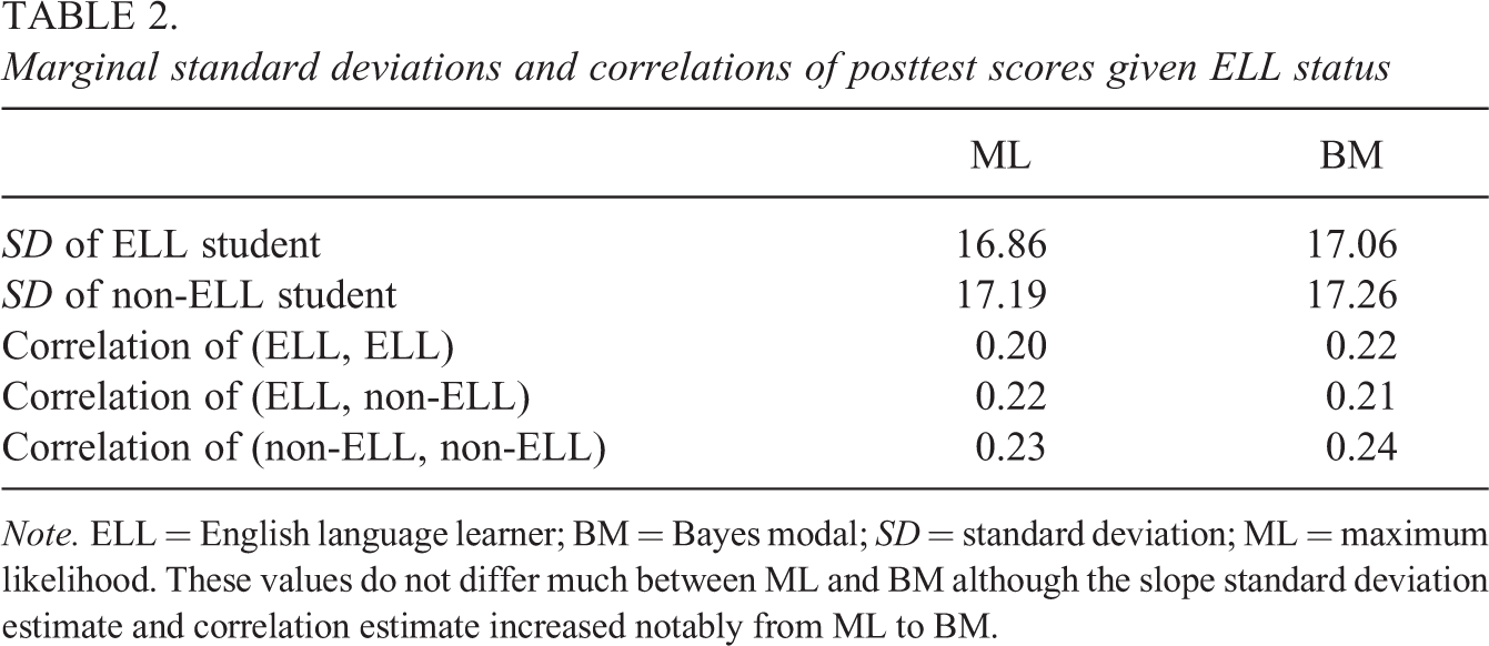
Note. ELL = English language learner; BM = Bayes modal; SD = standard deviation; ML = maximum likelihood. These values do not differ much between ML and BM although the slope standard deviation estimate and correlation estimate increased notably from ML to BM.
Simulation
We simulated data from the varying coefficient model as described in the preliminary simulation for Figure 1 but with only one covariate. We explored different values of the correlation ρ(0, 0.225, 0.450, 0.675, and 0.900), setting σ to be a moderate value of 0.5. With 1,000 replicated samples generated with J = 5 and n = 30, we estimated the bias and root mean squared error (RMSE) for σ1, σ2, and ρ. For ML and REML, the bias and RMSE of
Figure 7 shows the proportion of boundary estimates of
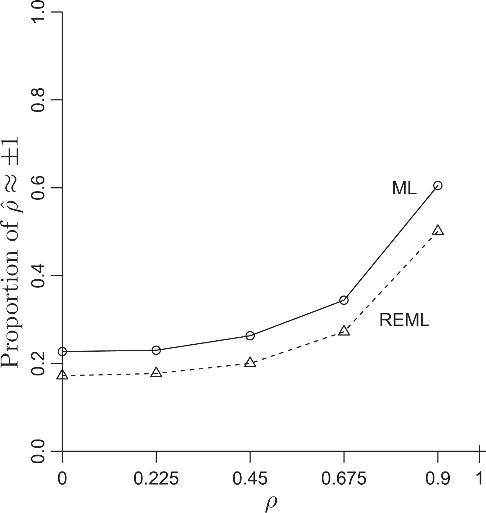
Proportion of maximum likelihood (ML) and restricted maximum likelihood (REML) estimates of ρ that are on the boundary. When ρ = 0, 21% of the ML estimates and 17% of the REML estimates are ±1. As ρ increases, the proportion of estimates on the boundary,
In spite of the absence of boundary estimates, the log likelihood is not reduced substantially by using BM estimation. Investigating the difference in deviances
Figure 8 summarizes the estimated bias and RMSE of
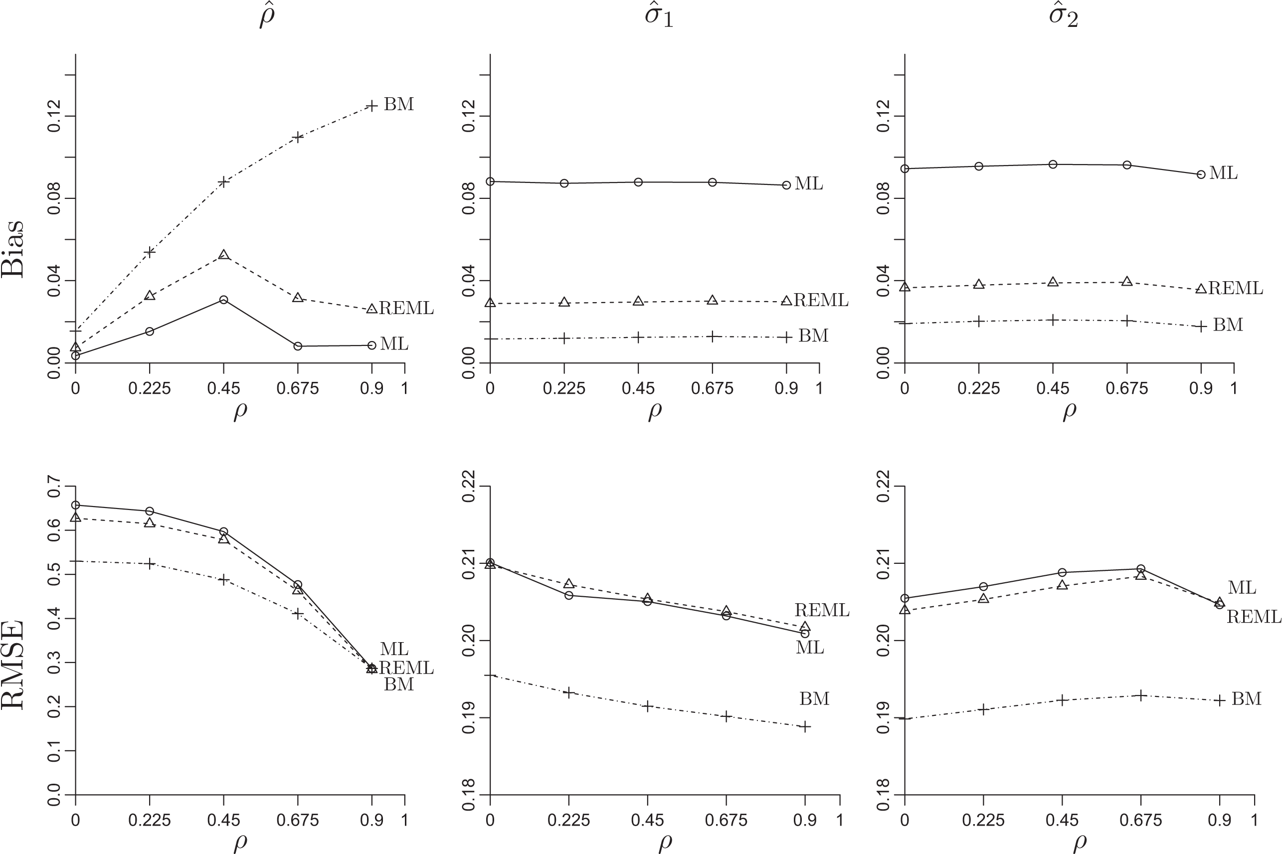
Bias and root mean squared error of
ML, REML, and BM all have some bias in estimating ρ, with BM having the most bias (i.e., the most shrinkage toward 0), as would be expected given the regularization from the Wishart prior that squeezes
The coverage of 95% confidence intervals for β0 and β1 does not change much with ρ. The average coverage of the BM confidence intervals is .940 for β0 and .943 for β1. The coverage for REML is about the same as that for BM, whereas ML shows slightly lower coverage with averages of .935 for β0 and .937 for β1.
Conclusion
For the hierarchical regression model, particularly with several varying coefficients, degenerate covariance matrix estimates do not have a practical interpretation. Unfortunately, such boundary estimates commonly arise in ML estimation because there is often little information on these parameters when there is only a moderate number of groups. In addition, when
In varying-slope models, changing the location and scale of the covariates that have varying slopes implies that Σ must change to produce an equivalent model. For example, for longitudinal data, we might want to transform the time variable to have a value 0 at the initial time point. In this case, subtracting a constant from the covariate changes the variance of the varying intercepts and the correlation between intercepts and slopes. Although ML and REML will yield equivalent models after linearly transforming the covariate, this is no longer true for BM estimation, which pulls the correlation toward 0. When using Bayesian regularization in this setting, it therefore becomes more important to choose meaningful centering points for the covariates with varying coefficients.
Footnotes
Authors’ Note
The data from Math Pathways and Pitfalls Lessons on Students Mathematics Achievement study are Copyright ©2011 by WestEd. All rights reserved. Any opinion, findings, and conclusions or recommendations expressed in this material are those of the author and may not reflect the views, findings, or opinions of the National Science Foundation or WestEd.
Declaration of Conflicting Interests
The authors declared no potential conflicts of interest with respect to the research, authorship, and/or publication of this article.
Funding
The authors disclosed receipt of the following financial support for the research, authorship, and/or publication of this article: The research reported here was supported by the Institute of Education Sciences (R305D100017), the National Science Foundation (SES-1323977), and the Army Grant (W911NF-14-1-0020). This data set is based upon work supported by the National Science Foundation under Grant No. 9911374 along with materials developed by WestEd.