
Abstract
Recently, there has been an increase in the number of cluster randomized trials (CRTs) to evaluate the impact of educational programs and interventions. These studies are often powered for the main effect of treatment to address the “what works” question. However, program effects may vary by individual characteristics or by context, making it important to also consider power to detect moderator effects. This article presents a framework for calculating statistical power for moderator effects at all levels for two- and three-level CRTs. Annotated R code is included to make the calculations accessible to researchers and increase the regularity in which a priori power analyses for moderator effects in CRTs are conducted.
In the past 15 years, there has been a strong shift toward the use of randomized trials (RTs), and specifically cluster RTs (CRTs), to evaluate the impact of educational programs and interventions. In CRTs, intact clusters (e.g., schools) are assigned to treatment conditions rather than individuals (e.g., students). CRTs are frequently an effective way to study interventions because they permit researchers to accommodate existing school structures and interventions that are designed to operate at the school level (Spybrook & Raudenbush, 2009). In order to yield rigorous evidence of whether a program works, however, such studies must be carefully designed. A principal consideration in the design of CRTs is the power or probability with which a study can detect effects if they exist.
The body of literature on statistical power for CRTs has largely focused on detecting average/main effects of treatment. A sizable number of articles and books have been published on this topic (i.e., Bloom, 1995; Donner & Klar, 2000; Hedges & Rhoads, 2009; Konstantopoulos, 2008; Liu, 2014; Murray, 1998; Raudenbush, 1997; Raudenbush & Liu, 2001; Schochet, 2008). The designs covered include two- and three-level CRTs as well as blocked or multisite CRTs (MSCRTs). This body of literature has clearly established that (1) the number of clusters is more influential than the number of individuals per cluster in terms of increasing the power of a study to detect the main effect of treatment of a given magnitude; (2) the more variability in the outcome across clusters, the greater the number of clusters needed; and (3) including a cluster-level covariate that is highly correlated with the outcome is often a cost-effective and efficient strategy for increasing the power.
Conducting the power calculations for the main effect of treatment for CRTs has also become much easier. Standard statistical software programs, for example, SAS Version 9.4, allow users to conduct power calculations for CRTs using procedures for mixed models (Littell, Milliken, Stroup, Wolfinger, & Schabenberger, 2006). In addition, several stand-alone programs for power calculations for CRTs exist including Optimal Design Plus (Raudenbush et al., 2011), CRT Power (Borenstein & Hedges, n.d.), and PowerUp! (Dong & Maynard, 2013).
A priori power calculations for the main effect of a treatment help ensure the study has the capacity to address the “what works” question. However, there is a growing recognition that there are important explanatory questions that need to be addressed if we are to fully understand the validity and value of substantive theories and interventions in education. One critical line of inquiry that is largely missing in conventional study designs concerns treatment effect moderation—or questions examining “for whom and under what circumstances” an intervention works. For example, it may be that an intervention is more effective in urban schools compared to rural schools or for girls compared to boys, such that school or individual characteristics moderate the treatment effect. Understanding the context in which an intervention is likely to be effective is fundamental to understanding the extent to which results are scalable and applicable to a wide range of schools and students.
The importance of studying moderation has gained considerable momentum in the field. For instance, in 2012, the conference theme for the annual meeting of the Society for Research on Educational Effectiveness was Understanding Variation in Treatment Effects and highlighted the importance of understanding how to design studies to enable them to better assess heterogeneity of treatment effects. Moderator effects that measure the treatment effect difference between subgroups represent one type of heterogeneous treatment effect. More recently, funders have started to strongly recommend a priori power analyses for tests of moderator effects (Institute of Education Sciences, 2016, p. 60). However, the literature for conducting power analyses for moderator effects in CRTs is less developed than for main effects.
Much like the case of power for the main effect of treatment in CRTs, the classic experimental design literature provides a framework for power calculations for moderator effects in CRTs. For example, one could consider a two-level CRT with a moderator at the individual level as a split-plot design with treatment as a whole-plot factor and the individual-level moderator as a split-plot factor (Littell et al., 2006). However, as evidenced by the large literature on power for main effects for CRTs, the reformulation of such designs within the familiar purview of hierarchical or multilevel models is prominent in education. This reframing facilitates direct connections among multilevel designs, hypothesis testing, and multilevel models that reduce power calculations to principles that are more concrete and accessible to researchers. Such restructuring has promoted a more informed appreciation for the factors that govern power and led to more reasonable approximations of power in recent CRTs (e.g., Spybrook & Raudenbush, 2009). Hence, it is critical to present power calculations for moderator effects within the context of CRTs and multilevel models and directly connect them to power calculations for the main effect. Only a handful of articles have done this. Raudenbush and Liu (2001) derive power formulas for site-level moderator effects for multisite trials in which individuals are randomly assigned within sites. Bloom (2005) and Jaciw (2014) focus on two-level CRTs with a binary Level 1 or Level 2 moderator. They provide formulas for the minimum detectable effect size difference (MDESD) or the smallest effect size difference that can be detected with power set to 0.80. Spybrook (2014) provides empirical estimates of the power of a set of funded CRTs to detect moderator effects but does not delineate an approach to estimate the power to detect moderation within the context of CRTs.
Statistical software options for calculating power for moderator effects for CRTs are also more limited than for power for the main effect. For example, none of the three most widely used programs for calculating power for CRTs, Optimal Design Plus (Raudenbush et al., 2011), CRT Power (Borenstein & Hedges, n.d.), or PowerUp! (Dong & Maynard, 2013), have specific functionality for calculating power for testing moderation.
The purpose of this article is to extend the literature and the tools available for power analyses for moderator effects in nested CRTs. As mentioned above, Bloom (2005) and Jaciw (2014) present MDESD formulas for the two-level CRT. We extend this work to power calculations for binary moderators at any level in a three-level CRT. We also implement the power formulas for moderator effects for the two-level and three-level CRT through two user-friendly tools to facilitate the use of these power formulas in planning CRTs. The tools include annotated R code and implementation of the formulas in PowerUp! 1 (http://www.causalevaluation.org/). We expect these tools will help make this work accessible to education researchers and increase the regularity in which a priori power analyses for moderator effects in CRTs are conducted.
The article is organized as follows. We begin with the model for a two-level CRT and briefly walk through the power calculations for the main effect of treatment. This is for pedagogical purposes, as it allows us to anchor notation and concepts in the more familiar power analyses for the main effect of treatment and directly transfer these to the less familiar power analyses for moderator effects. Next we provide the model and tests for a cluster-level and individual-level moderator in a two-level CRT and three-level CRT for balanced designs. To make direct connection among the approaches, we purposefully unpack and connect the models, test statistics, and noncentrality parameters. Then we extend to the case of unbalanced designs. Next we present several practical and deliberate examples of how to conduct a power analysis for different moderator effects. In the concluding section, we summarize the key components of the power calculations, explore the results and the implications of powering for moderator effects in the design of two- and three-level CRTs, and discuss future directions for this work.
Two-Level CRTs
Main Effect of Treatment
Suppose a team of researchers are planning a two-level CRT with students nested within schools and treatment assigned at the school level. Mathematics achievement is the outcome of interest. The Level 1 or student-level model is

where Yij is the math achievement for individual i = {1, …, n} in school j = {1, …, J}, β0j is the mean math achievement for school j, and eij is the residual error associated with students with variance σ2.
The Level 2 model or cluster-level model is

where γ00 is the grand mean math achievement; γ01 is the mean difference between the treatment and control group or the main effect of treatment; Tj is a treatment indicator, with −½ for control and ½ for treatment; and r0j is the residual error associated with schools with variance τ00. We assume equal allocation of clusters to treatment and control.
The treatment effect is estimated by

Note the variance is a function of the within-cluster variance, σ2; the between-cluster variance, τ00; the sample size within cluster, n; and the total number of clusters, J. The 4 is a result of J/2 clusters per condition, since we are assuming a balanced design. 2
In this case, we are testing H0: γ01 = 0. The power for the test is (Kirk, 1982)
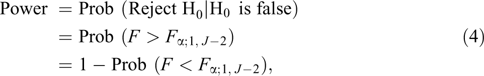
where F is the
If the null hypothesis is true, then the F-statistic follows the central F-distribution. If the null hypothesis is false, then the F-statistic follows the noncentral F-distribution with a noncentrality parameter, λ. The noncentrality parameter is a ratio of the squared main effect of treatment to the variance of the estimated treatment effect, as shown in Equation 5
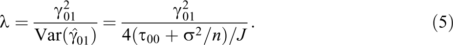
As the noncentrality parameter increases, the power increases. Thus, for the main effect of treatment in a two-level CRT, increasing the total number of clusters, J, has a greater effect on increasing power than increasing the total number of individuals per cluster, n, holding everything else constant. Note that it is common to standardize the parameters and reexpress λ as
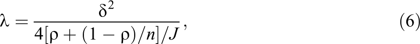
where
Before we move to the cluster-level moderator, we outline the extension for the main effect of treatment to the case with a cluster-level covariate. It is common practice to include a cluster-level covariate in the design of a CRT in order to increase the precision of the estimate (Raudenbush, Martinez, & Spybrook, 2007). Although an individual-level covariate may also be included, we focus on the cluster-level covariate because this directly reduces the between-cluster variance and is often more readily available and less expensive to collect than an individual-level covariate (Bloom, Richburg-Hayes, & Rebeck-Black, 2007). In this case, the Level 2 model is

The proportion of Level 2 variance explained by the covariate W is
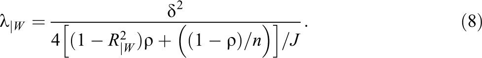
Note that the cluster-level covariate cannot reduce the variance at Level 1 since it is the same within clusters.
Cluster-level moderator
Suppose that the pool of schools in the previous study includes different types of schools, such as urban and rural schools. The research team suspects that the treatment effect may differ in urban schools compared to rural schools. Hence, they are interested in whether type of school, urban or rural, moderates the treatment effect. For illustrative purposes, suppose half the schools in the study are urban and half are rural and that they are equally allocated across conditions. The Level 1 model is identical to Equation 1. The Level 2 model or cluster-level model is

where γ00 is the grand mean; γ01 is the mean difference between the treatment and control group; Tj is a treatment indicator, with −½ for control and ½ for treatment; Sj is a school type indicator, with −½ for urban and ½ for rural; γ02 is the school type effect, γ03 is the Treatment × School Type interaction; and r0j is the residual error associated with clusters with variance τ00|S. The proportion of Level 2 variance explained by the moderator S and the interaction of S and T is
The moderator effect is estimated by

Note that the 16 in front is a function of the fact that there are now J/4 clusters per condition since there are now four conditions, rural experimental, urban experimental, rural comparison, and urban comparison.
The power for the cluster-level moderator effect, γ03, is an extension of the power for the main effect of treatment. The hypothesis of interest in this case is H0: γ03 = 0, the F-statistic is a ratio of MS T:S , which is the mean squares for the interaction, to the MS C , the degrees of freedom for the test are J − 4, and the noncentrality parameter, λ|S is the ratio of the squared treatment effect to the variance of the estimated moderator effect
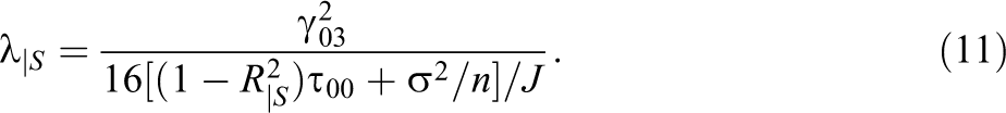
For consistency with main effect calculations, we standardize by setting τ00 + σ2 = 1. Hence, the noncentrality parameter using standardized notation is
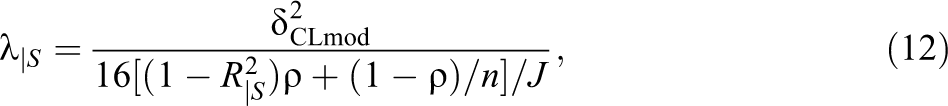
where
As discussed above, it is common to include a cluster-level covariate to increase precision, thus the new Level 2 model is

The addition of the cluster-level covariate further reduces the Level 2 variance where
Similar to the main effect of treatment, it is clear that the total number of clusters is the key sample size for increasing the power to detect cluster-level moderator effects. However, there are also important differences in the noncentrality parameters in Equations 7 and 14. First, the multiplier in the variance of the estimated treatment effect is 4 times larger for the moderator effect. This is a result of having J/4 clusters per condition rather than J/2 clusters per condition. Second, the set of covariates being conditioned on differs. For main effects, we condition on cluster-level covariate(s), whereas for moderator effects, we condition on the cluster-level covariate(s) and the moderator. Third, the numerator is a standardized differential treatment effect rather than a main effect. We briefly consider the role of these three factors before we move to the individual-level moderator.
First, consider the case in which,
Next, suppose that
Individual-level moderator
We might be interested in whether gender moderates the treatment effect. The Level 1 model or student-level model is now

where Yij is the math achievement for individual i = {1, …, n} in school j = {1, …, J}; β0j is the mean achievement in school j; Xij is an indicator for gender, with −½ for boys and ½ for girls; β1j is the gender gap in school j; and eij is the residual error associated with students. Note that gender explains the variation at Level 1 such that

where γ00 is the mean achievement across schools; Tj is a treatment indicator, with −½ for control and ½ for treatment; γ01 is the average treatment effect; γ10 is the gender gap; γ11 is the Treatment × Gender interaction; and r0j is the error associated with mean achievement across schools with variance τ00. Note we do not allow the gender gap to vary randomly across schools, although the model could be modified to reflect a random gender gap.
The individual-level moderator effect is estimated by

Similar to the case of a cluster-level moderator, the 16 in front of the variance is a function of the four groups, girls in treatment, boys in treatment, girls in comparison, and boys in comparison. However, unlike the variance for the cluster-level moderator effect, the between-school variance, τ00, does not contribute to the variance of the estimated moderator effect. This is because the differences in boys and girls are within schools and hence school effects cancel out.
The hypothesis of interest in this case is H0: γ11 = 0, the F-statistic is a ratio of MS T:X , which is the mean squares for the interaction effect, to the MS C with degrees of freedom n × J − J − 2. Given that the noncentrality parameter is a ratio of the squared treatment effect to the variance of the estimated treatment effect, it can be expressed as
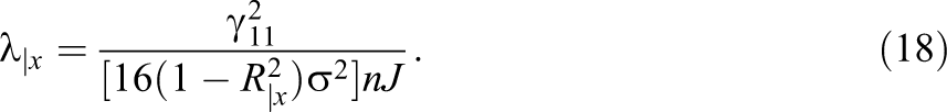
In order to be able to compare results with the power for the main effect of treatment and cluster-level moderators, we standardize the same way as above
where
There are important differences in the noncentrality parameter for the individual-level moderator compared to the noncentrality parameters for main effect of treatment and the cluster-level moderator. The key difference is that the between-cluster variance is not a part of the denominator for individual-level moderator effects. As a result, the number of individuals per cluster becomes as important as the total number of clusters. This differs from the main of treatment and the cluster-level moderator effect where the number of individuals per cluster was less critical and the number of clusters was the key sample size.
Before we move to the three-level case, we briefly summarize the key findings from the two-level case. From a sample size perspective, the total number of clusters is the most influential sample size for increasing the power to detect the main effect of treatment and a cluster-level moderator effect. However, the variance of the cluster-level moderator effect can be up to 4 times as large as the main effect of treatment which means many more clusters are necessary in order to detect a treatment effect of the same magnitude. Given that moderator effects tend to be smaller than main effects and education CRTs are typically designed to detect the main effect, the potential to design education CRTs with the capacity to detect cluster-level moderator effects of a reasonable magnitude may be limited. The situation is much more optimistic for designing two-level CRTs to detect individual-level moderator effects. This is a result of two factors: the between-school variance does not impact the power calculations and the number of individuals per cluster is equally as important as the total number of clusters. Hence, for a fixed total number of clusters, while increasing the number of individuals per cluster will not yield measurable gains for the power to detect the main effect of treatment or the cluster-level moderator effect, it has the potential to yield important gains in the power for the individual-level moderator effect.
Three-Level CRT
Main Effect of Treatment
Next we extend the work to the case of a three-level CRT. Suppose the same team of researchers are considering including a middle level in the study, teachers, so that they have a three-level CRT with students nested within teachers nested within schools. Math achievement remains the outcome of interest. The Level 1 or student-level model is

where Yijk is the math achievement for individual i = {1, …, n} in teacher j = {1, …, J} in school k = {1, …, K}; π0jk is the mean math achievement for teacher j in school k; and eijk is the error associated with students with variance σ2. The Level 2 or teacher-level model is

where β00k is the mean math achievement for school k and r0jk is the error associated with teachers with variance τπ. The Level 3, or school-level model is

where γ000 is the grand mean math achievement; γ001 is the mean difference between the treatment and control group or the main effect of treatment; Tk is a treatment indicator, with −½ for control and ½ for treatment; and u00k is the error associated with schools with variance τβ00. We assume equal allocation of clusters to treatment and control.
The treatment effect is estimated by

The hypothesis of interest is H0: γ001 = 0, the F-statistic is a ratio MS T to the MS C , the degrees of freedom for the test are K − 2, and the noncentrality parameter is

Like in the case of the two-level CRT, it is common to standardize the parameters such that

where
It is also typical to include a school-level covariate to increase the power of the study. Assuming a school-level covariate, such as school-level pretest, the Level 3 variance will be reduced by

School-level moderator
Again we assume that half the schools in the study are urban and half are rural and that they are equally allocated across conditions. The Level 1 and Level 2 models are identical to Equations 20 and 21. The new Level 3 model is

where γ000 is the grand mean math achievement; γ001 is the mean difference between the treatment and control group; Tk is a treatment indicator, with −½ for control and ½ for treatment; Sk is a school type indicator, with −½ for urban and ½ for rural; γ002 is the school type effect; γ003 is the Treatment × School Type interaction or the school-level moderator effect; and u00k is the residual error associated with schools. Note that where
The moderator effect is estimated by

The hypothesis of interest in this case is H0: γ003 = 0, the F-statistic is a ratio of MS T:S to the MS C , the degrees of freedom for the test are K − 4, and the noncentrality parameter, λ|S, is
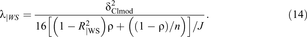
Hence, the noncentrality parameter using standardized notation is

where
Note that we could also include a cluster-level moderator, W, where
Teacher-level moderator
Given the three levels, we can also test for moderator effects at the teacher level. For example, teacher experience may moderate the effect of the intervention. Assume that teacher experience is quantified as new teacher (teaching 0–5 years) or veteran teacher (teaching more than 5 years). The Level 1 model remains the same as in Equation 20. The new Level 2 or teacher-level model is

where β00k is the mean math achievement for school k; Mjk is an indicator for teacher experience, with −½ for 0–5 years, or new teacher, and ½ for more than 5, or veteran teacher; β01k is the teacher experience gap in school k; and r0jk is the residual error associated with teachers. Note that we assume that percentage of variance explained by teacher variance is

where γ000 is the grand mean math achievement; γ001 is the mean difference between the treatment and control group; Tk is a treatment indicator, with −½ for control and ½ for treatment; γ010 is the teacher experience gap; γ011 is the Treatment × Teacher Experience interaction; and u00k is the residual error associated with schools with variance τβ00. Note that we do not allow the experience gap to vary randomly across schools, although this assumption could be relaxed.
The parameter of interest is γ011. The moderator effect is estimated by

The F-statistic in this case though is a ratio MS T:M , which is the mean squares for the interaction to the MS C with J × K − J − 2 degrees of freedom. The noncentrality parameter is defined as
where
Note that the between-school variance does not enter the calculations for the power of the teacher-level moderator, as the difference between new and experienced teachers is within schools. The teacher-level variance and student-level variance are the only two variance components that affect the power. Hence, the number of teachers per school becomes a much more critical sample size in the power calculations.
Individual-level moderator
We might also be interested in whether gender moderates the treatment effect in a three-level CRT. The Level 1 model or student-level model is now

where Yijk is the math achievement for individual i = {1, …, n} in teacher j = {1, …, J} in school k = {1, …, K}; π0jk is the mean achievement for teacher j in school k; Xijk is an indicator for gender, with −½ for boys and ½ for girls; π1jk is the gender gap for teacher j in school k; and eij is the residual error associated with students. The percentage of variance explained by gender is

where β00k is the mean achievement across schools; r00k is the error associated with mean achievement across teachers in schools with variance τπ. Note we do not allow the gender gap to vary randomly across teachers in schools. The new Level 3 model is

where γ000 is the grand mean achievement; Tk is a treatment indicator, with −½ for control and ½ for treatment; γ001 is the overall treatment effect; γ100 is the gender gap; γ101 is the Treatment × Gender interaction; and r00k is the error associated with schools with variance τβ00 .
The moderator effect of interest is γ101, which is estimated by

The F-statistic in this case though is a ratio MS T:X to the MS C with n × J × K − J × K − K − 2 degrees of freedom and the noncentrality parameter is defined as

where
Note that because the moderator is at Level 1 and hence the difference between boys and girls is within teacher, the between-teacher and between-school variance components are removed from the variance of the moderator effect. Hence, the number of individuals per cluster is a critical sample size in power calculations for the individual-level moderator effect in a three-level CRT.
The three-level CRT is a natural extension of the two-level CRT and findings are similar. That is, for the main effect and the school-level moderator, the power is most heavily influenced by the total number of clusters. In addition, designing a study to detect a school-level moderator will require many more clusters than designing a study to detect the main effect of treatment since the moderator effect will likely be smaller and the variance of the estimated moderator effect may be up to 4 times that of the main effect. As we consider lower level moderators, the sample size at the level of the moderator becomes more important. That is, for a teacher-level moderator, the number of teachers is as important as the total number of schools, given that the between-school variance is removed. Further, for a student-level moderator, the number of students is as influential as the number of teachers per school and the total number of schools because the between-teacher and between-school variance components are removed from the moderator effect.
Unbalanced Designs
Thus far, we have assumed perfectly balanced designs. For example, in a two-level CRT with 40 total schools we assumed the ideal case, 20 schools in treatment and 20 schools in control, and 10 rural and 10 urban school in each condition. Given this structure, we maximize the power for both the test of the main effect and the cluster-level moderator.
However, in practice, it may not always be feasible to achieve a perfectly balanced design. For example, suppose that in order to increase the likelihood of schools participating in a study, the researchers plan to assign 28 schools to the treatment condition and 12 to the control condition. We can use the same formulas described above for the test of the main effect of treatment by replacing the total number of clusters with the effective sample size for the calculations. In this case, the effective sample size is 2 times the harmonic mean (HM). The HM of the treatment and control conditions is
The same process can be used for the moderator power calculations. However, now we need the HM of the four groups: rural treatment, urban treatment, rural control, and urban control. Suppose that of those 28 treatment clusters, 14 are rural schools and 14 are urban schools, and of the 12 control clusters, 6 are rural schools and 6 are urban schools. The HM of the four groups is
The logic of this example is applicable for any of the power calculations discussed in this article and can be applied as follows: First, identify the estimator for the effect of interest. Second, identify the sample size for each of the groups included in the estimator. If they are not equal, calculate the HM for each group. For power calculations, for the main effect of treatment, double the HM to calculate the total effective sample size that will be used for the calculations. For power calculations, for the moderator effects, calculate the HM for each of the four groups and multiply it by four for the effective sample size that can be used for the calculations. The effective total sample size for the power calculations may be different for the main effect and the moderator effects depending on the allocation of clusters and individuals.
It is important to note that in practice the sample sizes for the different moderator variables may be beyond the control of the researcher. For example, there may not be an equal number of boys and girls in a class, or new and experienced teachers within a school, or rural and urban schools in the sample of schools willing to participate in the study. As the imbalance increases, the power to detect an effect of a given magnitude will decrease. Hence, to the extent possible, it is important to identify moderators of interest prior to recruiting for a study and to consider these variables during the recruitment process.
Examples
We begin with an example of a two-level CRT. Continuing with the idea of mathematics achievement as the primary outcome, suppose that based on past studies of the intervention, a team wants to design a study to detect a main effect of treatment that has a standardized effect size of 0.20. They plan to test the intervention in urban and rural schools and are interested in whether the treatment effect is moderated by school type. Recognizing that the moderator effect will be smaller than the main effect of treatment, they are interested in detecting a cluster-level moderator effect of 0.10. Suppose the team is limited to a total of 40 schools, 20 urban and 20 rural, with 100 students per school. Assume that they assign 20 schools to each condition and that the number of urban and rural schools in each condition is balanced. Note that this assumption could be relaxed to allow for imbalance in groups in which case the HM calculations described above would apply. Based on the literature (Hedges & Hedberg, 2009, 2014), they estimate an ICC of 0.23. They have access to a school-level covariate, last year’s scores, and assume an
Figure 1 shows the power to detect the main effect of treatment of 0.20 and the cluster-level moderator of 0.10. As expected, the power for the main effect of treatment is always greater than the power for the cluster-level moderator. Assuming 40 total clusters, the power to detect the main effect of treatment in this case is 0.56. In order to reach the acceptable level of 0.80, they would need an additional 30 clusters for a total of 70. The power to detect the cluster-level moderator effect of 0.10 for 40 total clusters is only 0.09. Assuming 70 total clusters, the number needed to reach adequate power for the main effect of treatment, the power is still only 0.13 for a cluster-level moderator of 0.10. It is clear that the number of clusters to achieve adequate power for the cluster-level moderator will be outside a reasonable range.
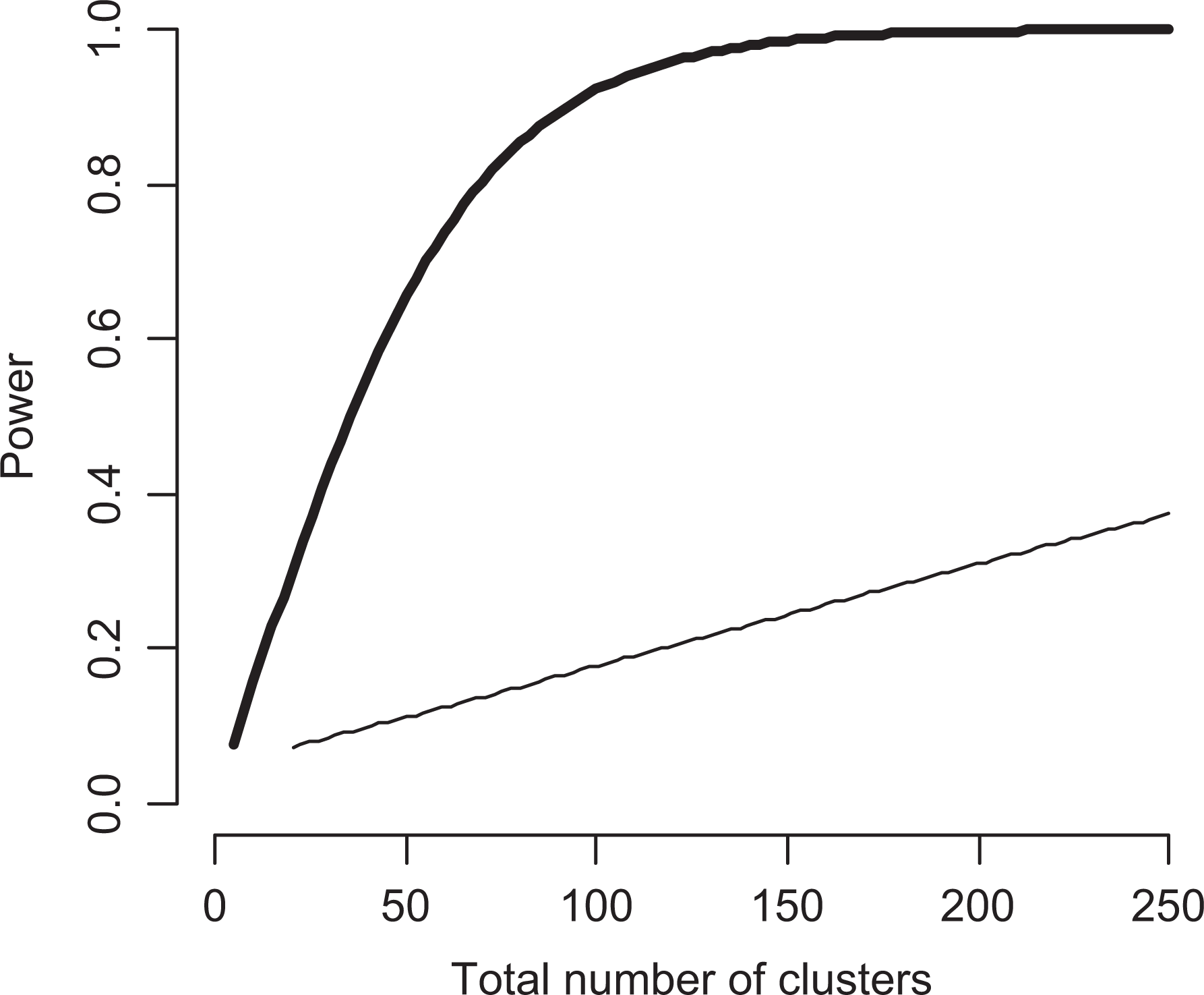
Power curves for main effect of treatment and cluster-level moderator.
Suppose that a different team of researchers are also designing a study of the same intervention. They were concerned that the treatment effect may have a differential effect on boys and girls, hence they are interested in power the study to detect an individual-level moderator effect in addition to the main effect of treatment. They seek to detect an individual-level moderator effect of 0.10. Assuming the same design parameters as above, a total of 40 schools, 100 students per school (assuming half girls and half boys), an ICC = 0.23, and an
The three-level CRT follows the same pattern as the two-level CRT. That is, the power for the main effect of treatment and the school-level moderator is driven by the total number of clusters or schools. The power for the lower level moderator effects is also strongly influenced by the sample size of the moderator of interest. For example, Table 1 displays the power to detect the main effect of treatment, cluster-level moderator, teacher-level moderator, and individual-level moderator under the following assumptions: main effect of treatment of 0.20, school-level moderator effect of 0.10, teacher-level moderator effect of 0.10, student-level moderator effect of 0.10, a total of 40 schools, either 5 or 30 teachers per schools, either 10 or 30 kids per teacher, an ICC at the school level of 0.15, an ICC at the teacher-level of 0.08,
Power for Main Effect, Cluster-Level Moderator, Teacher-Level Moderator, and Individual-Level Moderator Effects
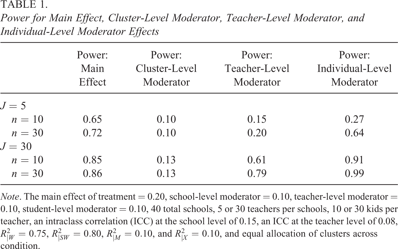
Note. The main effect of treatment = 0.20, school-level moderator = 0.10, teacher-level moderator = 0.10, student-level moderator = 0.10, 40 total schools, 5 or 30 teachers per schools, 10 or 30 kids per teacher, an intraclass correlation (ICC) at the school level of 0.15, an ICC at the teacher level of 0.08,
The table illustrates the effects of the sample sizes at different levels on different effects. For the main effect of treatment and the cluster-level moderator, the power is not strongly influenced by increases in the number of individuals per teacher or the total number of teachers per school. However, increasing the total number of teachers per school increases the power to detect a teacher-level moderator. The challenge with this is that, in many cases, the total number of teachers per school may be small, particularly if only one grade level is represented. For the individual-level moderator, it is clear that increasing for 10 to 30 students per teachers has a strong effect on the power, particularly in the case with a smaller total number of schools and number of teachers. For most elementary and middle/high schools, a per class sample size of 25 to 30 is quite common. The smaller sample sizes are more prevalent in pre-K studies that may make individual-level moderator effects more difficult to detect in these studies.
Discussion
The capacity of CRTs to provide rigorous evidence of the main effect of treatment has improved in the past decade. That is, more recent CRTs are being designed with adequate power to detect a meaningful main effect of treatment that past CRTs (Spybrook & Raudenbush, 2009). As we start to design studies that enable us to determine whether or not an intervention has an overall effect, we also begin to ask other important question regarding whether the effect is the same across different kinds of schools, teachers, and students. Hence, it becomes important to think about whether we can power CRTs to detect not only the main effect of treatment but also important moderator effects.
Some general patterns emerge from the findings related to the different types of moderator effects. For the purpose of this discussion, consider a two-level CRT with students nested within schools and a three-level CRT with students nested within teachers nested within schools. In both cases, powering for the school-level moderator effect will be challenging, given the current size of CRTs in the field. As illustrated by the formulas and in the examples, the power for a cluster-level moderator tends to be much smaller than the power for the main effect. Given that it is often challenging for teams to afford enough clusters to power for the main effect of treatment, the number of schools required to power for a cluster-level moderator is likely to be outside the budgetary constraints. This suggests that the analysis of school-level moderator effects may require a more meta-analytic approach involving combining across studies.
However, lower level moderator effects hold much more promise from a power perspective. In a three-level CRT with students nested in teachers nested in schools, designing studies to detect teacher-level moderators may be possible. That is, the power for teacher-level moderators is driven more by the number of teachers per schools as shown in the formulas and examples. For studies examining the effect of a whole school intervention in which randomization takes place at the school level and all teachers in the school are involved, it may be reasonable to design the study with adequate power to detect teacher-level moderators because the number of teachers per school may be large. This presents an important opportunity for researchers to be able to answer critical questions about teacher moderator effects that may help improve the likelihood an intervention is effective. For example, if the researchers determine that an intervention is more effective with experienced teachers rather than novice teachers, they may be able to put in additional professional development opportunities for less experienced teachers to help them overcome challenges.
The greatest potential for detecting moderator effects in CRTs lies in individual-level moderator effects. As we saw in both the two- and three-level CRT, the power for the individual-level moderator depends much more heavily on the number of individuals per cluster. In many CRTs in education, all of the students in a school or all of the students in a grade will participate in a study. This means that there are often large numbers of individuals per cluster. Taking advantage of the number of individuals per cluster and hence asking a priori questions about individual-level moderators can help researchers better understand for whom a program is effective. This is a critical step toward designing, developing, and implementing programs that meet the needs of all students. For example, suppose that a group of researchers testing a math curriculum are concerned that the program is less effective for English-language learners (ELL). In their sample, about half of the students are ELLs and hence they test whether ELL moderates the treatment effect. If findings suggest that there is a differential effect, the team can then explore how to modify the treatment, so that ELL and non-ELLs benefit from the program.
For many other K–12 studies, powering to detect an individual-level moderator of a reasonable magnitude may be a very realistic goal for the study. The exception to this case is when there are only a small number of individuals per cluster. For example, in pre–K classrooms, the number of students per class may be less than seven which would make powering the study to detect individual-level moderators very challenging.
Future Directions
In this article, we focused on clustered designs. Extending the work to MCRTs is critical, as multisite studies are quite common in evaluations of educational interventions. Furthermore, we discussed binary moderators in this article. Moderators can also be continuous in nature, for example, whether the program’s effect is moderated by school quality, and extending the work to continuous moderators is another critical step. We also fixed the moderator effects at lower levels. It may not always be the case that moderator effects are fixed and thus allowing the moderator effects to vary randomly is another area for future research. In addition, understanding more about the magnitude of moderator effects is a critical step toward planning studies appropriately. For example, how different is the effect on boys and girls? Or for urban schools versus rural schools? As we begin to develop empirical estimates of the magnitude of moderator effects, we can start to use these effect sizes to guide the power analyses.
Footnotes
Declaration of Conflicting Interests
The author(s) declared no potential conflicts of interest with respect to the research, authorship, and/or publication of this article.
Funding
The author(s) declared the following financial support for the research, authorship, and/or publication of this article: This project has been funded by the National Science Foundation [DGE-1437679, DGE-1437692, DGE-1437745]. The opinions expressed herein are those of the authors and not the funding agency.