
Abstract
Questionnaires that include items eliciting count responses are becoming increasingly common in psychology. This study proposes methodological techniques to overcome some of the challenges associated with analyzing multivariate item response data that exhibit zero inflation, maximum inflation, and heaping at preferred digits. The modeling framework combines approaches from three literatures: item response theory (IRT) models for multivariate count data, latent variable models for heaping and extreme responding, and mixture IRT models. Data from the Behavioral Risk Factor Surveillance System are used as a motivating example. Practical implications are discussed, and recommendations are provided for researchers who may wish to use count items on questionnaires.
Count data are prevalent in the behavioral and health sciences. Statistical methods for the analysis of univariate count outcomes have existed for several decades and are commonly variants of the log-linear model, including Poisson regression (e.g., Agresti, 2002; Cameron & Trivedi, 2013; McCullagh & Nelder, 1989), negative binomial regression (e.g., Hilbe, 2011), and their zero-inflated extensions (e.g., Lambert, 1992). These models have widespread application in fields such as psychology (e.g., Lewis et al., 2010), medicine (e.g., Roberts & Brewer, 2010), economics (e.g., Deb & Trivedi, 1997), among others. Loeys, Moerkerke, De Smet, and Buysse (2012) recently published a review of some of the current challenges and proposed solutions to modeling univariate count outcomes in psychological research.
Questionnaires that comprise multiple items eliciting count responses are becoming increasingly common, particularly in public health. Often, these surveys are designed to assess the severity of symptoms, asking respondents to recall the frequency of various thoughts or behaviors over a specified period of time. For example, a survey measuring alcohol dependence may ask the respondent to report the number of drinks he or she consumes during a typical week. While statistical methods for the analysis of a single count outcome are widely available, methods for modeling multivariate count outcomes on questionnaires are considerably less well-developed. One approach might be to modify traditional item response theory (IRT) techniques, invoking a log link function in place of the usual logit link and a Poisson distribution in place of a Bernoulli or multinomial conditional response distribution. However, if one examines most self-report count data more closely, a number of additional challenges surface that require a more complex methodological approach.
Figure 1 shows a histogram of responses to 4 items on the Behavioral Risk Factor Surveillance System (BRFSS; Centers for Disease Control and Prevention, 1984–present). These items ask respondents to report the number of days in the past 30 days they have experienced a specific symptom, thought, or behavior. It is clear from the histograms that the observed responses do not follow a standard count distribution (e.g., Poisson, negative binomial). Not only is there a very large proportion of respondents reporting 0 days, much larger than would be expected from a standard count distribution, but there is also a substantial proportion of respondents reporting the maximum of 30 days. Further, there is a noticeable inflation at days that are multiples of 5, an example of a phenomenon known as heaping in the biostatistics literature (e.g., H. Wang & Heitjan, 2008). Simple modifications to a conventional IRT model are not likely to account for the potential subpopulations and individual differences that manifest in Figure 1. This research attempts to address the challenges of modeling multivariate count data with inflation and heaping by combining methodological approaches from three distinct but related literatures: IRT models for multivariate count data (L. Wang, 2010), latent variable models for heaping (H. Wang & Heitjan, 2008) and extreme responding (Böckenholt, 2012; Bolt & Johnson, 2009; De Boeck & Partchev, 2012; Thissen-Roe & Thissen, 2013), and mixture IRT models (Finch & Pierson, 2011; Finkelman, Green, Gruber, & Zaslavsky, 2011; Sawatzky, Ratner, Kopec, & Zumbo, 2012; Wall, Park, & Moustaki, 2015).
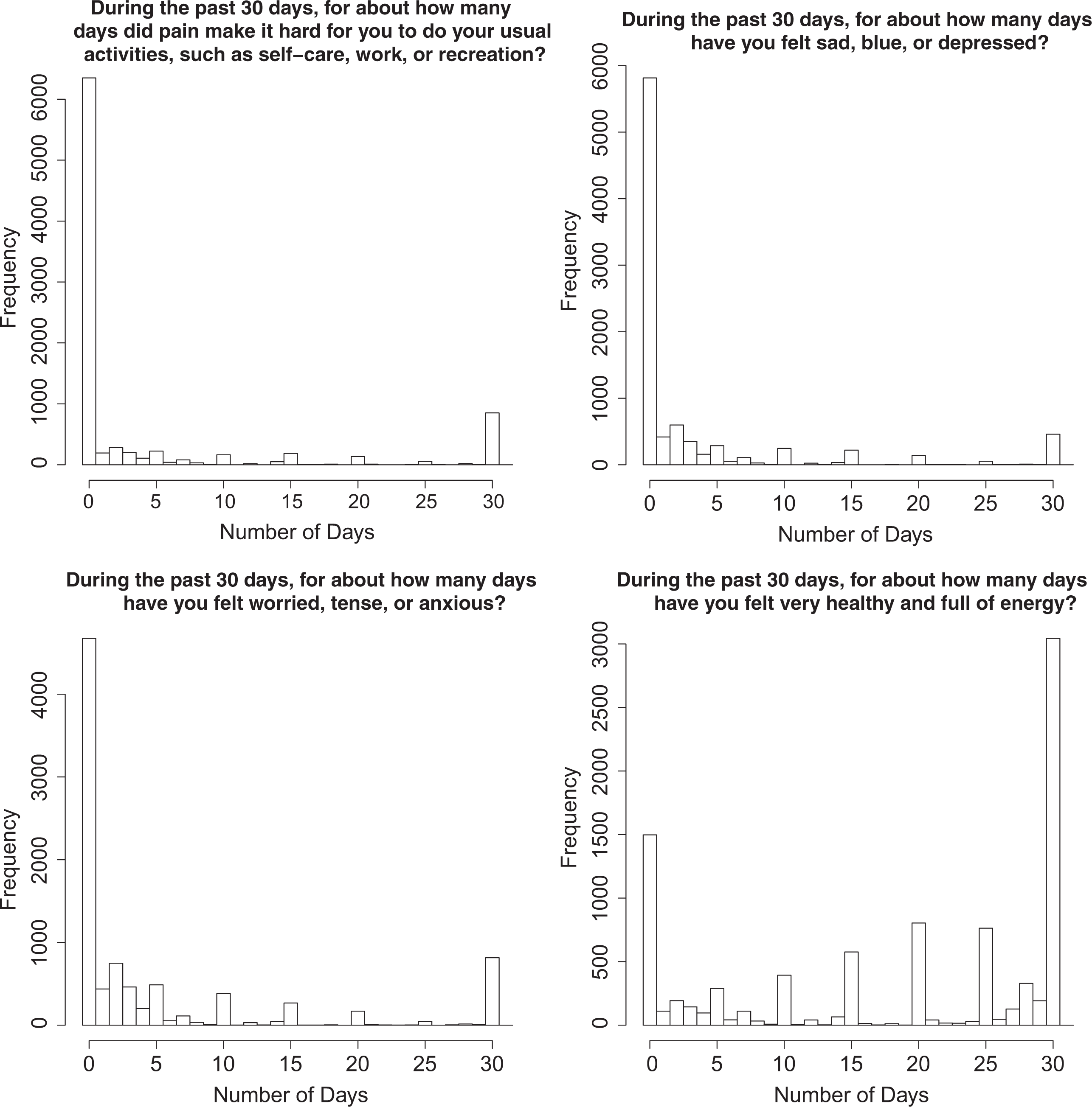
Frequency histograms for four general emotional health items from the Behavioral Risk Factor Surveillance System (2014) eliciting count responses.
Item Response Models for Multivariate Count Data
Several researchers have proposed psychometric models for multivariate count data (Böckenholt, Kamakura, & Wedel, 2003; L. Wang, 2010; Wedel, Böckenholt, & Kamakura, 2003). Perhaps most relevant for data like those from the BRFSS, L. Wang (2010) developed an IRT model for zero-inflated count data, highlighting its application to the analysis of substance use frequencies. Such data often exhibit zero inflation because a subset of respondents abstain from substance use and endorse zero for every item. Based on Lambert’s (1992) original zero-inflated Poisson regression model, Wang’s zero-inflated Poisson-IRT (ZIP-IRT) model is a latent variable mixture model that accounts for two different response processes: the zero process that relates to whether the event (i.e., alcohol consumption) has a chance of occurring at all and the Poisson process that relates to the expected count (i.e., number of alcoholic drinks consumed), given that the event has a chance of occurring. L. Wang (2010) uses a logit link function and Bernoulli conditional response distribution to model the probability of being in the Poisson process, and a log link function and Poisson conditional response distribution to model the expected count, given that someone is in the Poisson process. Each model component has a set of item discrimination and location parameters as well as a single latent variable that represents substance dependency.
While Wang’s model provides an item response modeling framework for analyzing the psychometric properties of zero-inflated multivariate count data, it assumes that the nonperfect zero state is a Poisson process. Real-world data analysis suggests that the Poisson distribution rarely describes observed count responses; this is especially true of retrospective self-report data in which heaping is present (e.g., H. Wang & Heitjan, 2008), as illustrated in Figure 1. For this reason, a more flexible modeling framework may be useful.
Heaping and Response Style
Modeling heaping in univariate count outcomes has been a subject of interest in the biostatistics literature (Heitjan & Rubin, 1990; Ridout & Morgan, 1991; H. Wang & Heitjan, 2008). To account for heaping and digit rounding in self-reported counts of cigarette use, H. Wang and Heitjan (2008) introduced a model in which the observed cigarette count is a function of both an unobserved true cigarette count and a latent class “heaping behavior” variable. Others have also developed models for heaping and data coarsening in univariate outcomes, such as rounding in self-reported age (Heitjan & Rubin, 1990), digit preference in retrospective reporting of women’s number of menstrual cycles before a positive pregnancy (Ridout & Morgan, 1991), and rounding in clinician-reported measurements from ultrasound images (Wright & Bray, 2003). These models have applications to univariate count outcomes; however, review of the biostatistics literature has not uncovered methods of accounting for heaping in multivariate count outcomes.
While the psychometrics literature does not include specific models for heaping in multivariate count data, research on extreme responding on surveys comprising Likert-type items addresses a similar concept within an IRT framework. Some have used multidimensional IRT models to account for an “extreme response style” (ERS) latent variable (Bolt & Johnson, 2009; Bolt & Newton, 2011). Bolt and Newton (2011) describe a multidimensional nominal response model (NRM) in which there is a latent variable related to the construct of interest as well as a latent variable for ERS. Others have approached the topic from a decision tree perspective, in which the observed responses manifest from a sequence of internal decisions (Böckenholt, 2012; De Boeck & Partchev, 2012; Thissen-Roe & Thissen, 2013). Böckenholt (2012) and De Boeck and Partchev (2012) propose a tree structure for capturing individual differences in response style, arguing that it is possible that more than one response process is at play when someone responds to a Likert-type questionnaire item. Thissen-Roe and Thissen (2013) adopt a similar view, positing that response direction and response intensity to Likert-type items can be modeled by two stage-like processes. Biostatistical models for heaping and psychometric models for extreme responding developed from different methodological frameworks; however, both approaches converge on the idea of a latent variable underlying individual differences in response style. The count response methodology from the biostatistics literature, coupled with the extreme responding methodology from the psychometrics literature, lay the groundwork for the development of an IRT model that can accommodate multivariate count responses that also exhibit heaping.
Mixture IRT
Unlike traditional IRT models, mixture IRT models assume that the observed responses are sampled from a population that has a number of distinct subpopulations (Rost, 1990, 1997; von Davier & Rost, 2006). Under the assumption of local independence, the marginal mixture distribution of the observed item responses
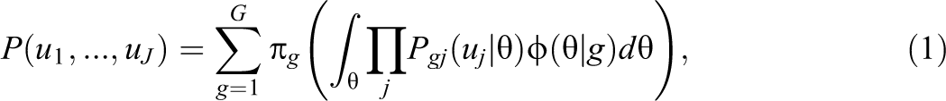
where
Mixture IRT has been applied to the analysis of substance use or risky behavior scales, where many of the items may not be applicable to substantial proportions of the population (Finch & Pierson, 2011; Finkelman et al., 2011; Muthen & Asparouhov, 2006; Sawatzky et al., 2012; Wall et al., 2015). Respondents belonging to one of the latent classes—for example, a subgroup of people who abstain from drinking but are nonetheless asked a series of questions relating to symptoms of alcohol dependence—may not engage with the items the same way as other subgroups in the population, and the mixture IRT modeling can help to account for both individual- and group-level differences.
When many of the respondents in the population possess none or very low levels of the construct being measured, such as a group of individuals not endorsing any of the criteria on a symptoms checklist, it is plausible that the latent variable follows a mixture distribution with a zero-inflated component. Such constructs are often referred to as “unipolar” (Reise & Waller, 2009; Wall et al., 2015). In clinical assessment, there may also be a smaller subset of respondents who are extreme at the other end of the latent variable, endorsing all possible symptoms on a checklist. Finkelman, Green, Gruber, and Zaslavsky (2011) referred to the high frequency of respondents with the maximum observed score as K inflation. To circumvent the challenges associated with measuring low-prevalence psychiatric disorders, Finkelman et al. (2011) developed a latent class IRT model to account for extreme subpopulations. One latent class describes individuals with no symptoms; the IRT model for this class is degenerate. A second latent class describes the people exhibiting all of the symptoms; the IRT model for this class is also degenerate. The remaining latent class, labeled the graded class, describes people along the severity continuum that is implied by a traditional IRT model with a normal population density. More recently, Wall, Park, and Moustaki (2015) proposed a similar model for measuring psychiatric disorder severity in a zero-inflated population. In both applications, the presence of respondents from a potentially heterogeneous population requires mixture IRT in place of an IRT model that assumes a normal population density.
The Proposed Latent Class IRT Model
A review of the literature suggests three methodological approaches for solving three distinct problems in measurement: zero-inflated Poisson psychometric models for the analysis of multivariate zero-inflated count data (L. Wang, 2010), latent variable models to account for heaping in univariate count outcomes (H. Wang & Heitjan, 2008) and extreme responding in multivariate Likert-type items (Böckenholt, 2012; Bolt & Johnson, 2009; Bolt & Newton, 2011; De Boeck & Partchev, 2012; Thissen-Roe & Thissen, 2013), and mixture IRT models for clinical assessment in heterogeneous populations (Finch & Pierson, 2011; Finkelman et al., 2011; Sawatzky et al., 2012; Wall et al., 2015). All three methods have utility in particular scenarios; however, we are unaware of any existing unifying framework for the analysis of multivariate count outcomes that also accounts for zero inflation, maximum inflation (K inflation), and heaping. This research borrows elements from all three methodological approaches in developing a latent class IRT model for multivariate zero-inflated count data that are sampled from a potentially heterogeneous population. To make the presentation concrete, we use as an illustration the responses to the four count items from the BRFSS that are shown in Figure 1.
According to the general latent class model, the unconditional probability of observed response uj to item j can be expressed
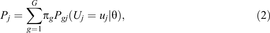
in which g denotes latent class membership, πg specifies the probability of belonging to latent class g, and
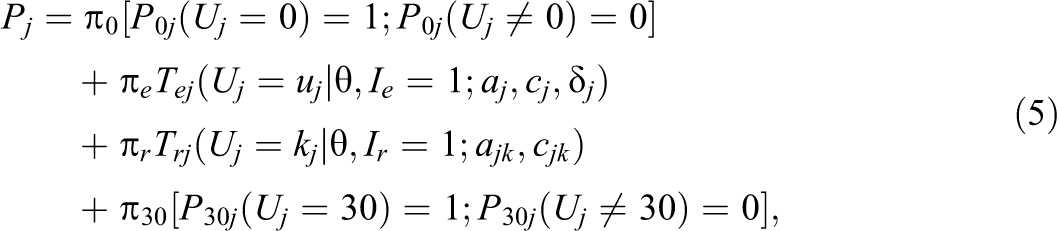
One latent class, with probability π0, describes some, perhaps many, of the people who respond 0 days to all 4 items with response vector
In addition to the zero and maximum classes, we propose two “graded” latent classes that describe people falling along the continuum of the latent variable. One graded class with probability πe is referred to as the exact count class and comprises the subset of people whose responses follow a standard count distribution. These are individuals who possess some level of the latent variable and report the exact number of days they experience a symptom, regardless of whether the counts are multiples of 5. To model the conditional probability of count response uj from members of the exact count class, we use a negative binomial IRT model to allow for overdispersion:
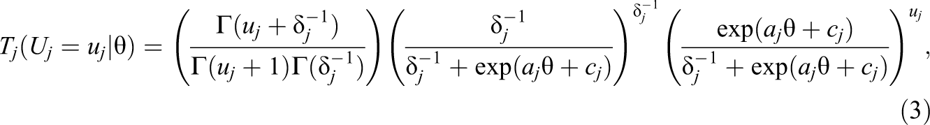
in which aj, cj, and δj are the discrimination, intercept, and overdispersion parameters for item j, respectively, and θ is the latent variable being measured by the 4 items. The larger the a parameter, the more effective the item is in separating individuals on the latent variable. The c parameter is the expected count for someone at the mean level of the latent variable (θ = 0).
The remaining latent class with probability πr is referred to as the rounding/selected response class; it includes individuals who respond only with counts that are multiples of 5. Instead of treating the item as having an open-ended count scale, these people treat the item as having a smaller, fixed number of response categories: {0,5,10,15,20,25,30}. To model the conditional probability of observing count response uj from members of the rounding/selected response class, an NRM can be used (Bock, 1972; Thissen, Cai, & Bock, 2010). The trace line for the NRM is expressed
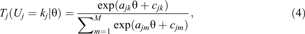
in which kj corresponds to the response category for item j. To avoid confusion with count response uj that can take on any nonnegative integer value up to 30, we adopt the alternative notation kj such that
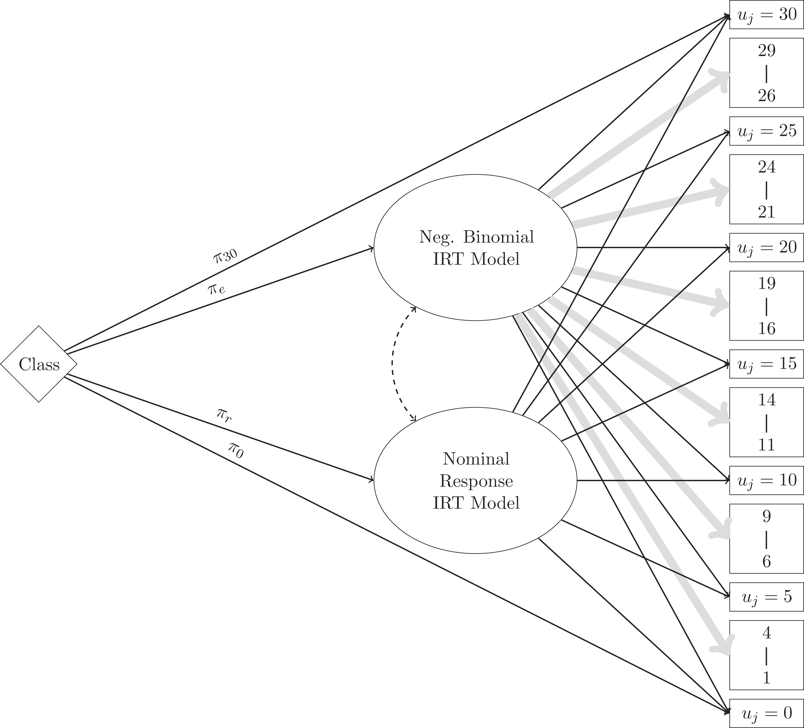
Tree diagram showing the proposed response processes. Consider an observed count of 0. The respondent may be a member of the zero class and select 0 days for every item; this option is represented by the direct path from the item to a zero response, without passing through either of the two item response theory (IRT) models. It is also possible that the person is a member of the exact count class and reports 0 days. This option is represented by the indirect path to the zero response through the negative binomial IRT model. It is also possible that the respondent is a member of the rounding/selected response class and reports 0 days. Instead of passing through the negative binomial IRT model, these individuals arrive at a zero response via the nominal response IRT model. Multiple potential internal processes also underlie the nonzero responses.
The Full Latent Class IRT Model
Let I0, Ie, Ir, and I30 be indicator variables denoting membership in the zero, exact count, rounding/selected response, and maximum classes, respectively, with probabilities π0, πe, πr, and
where
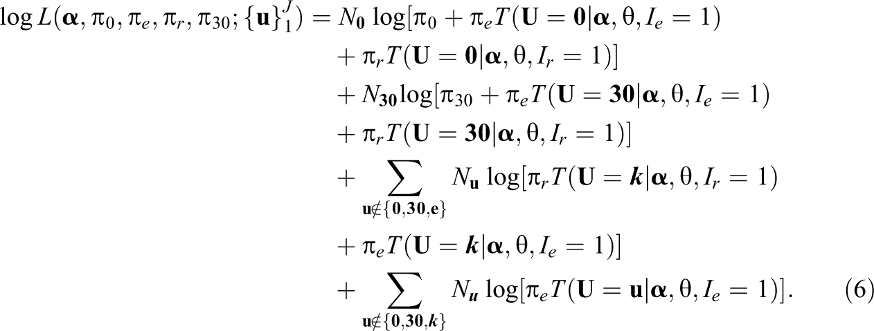
In Equation 6,
Parameter estimation for the latent class IRT model can done with maximum likelihood using nlm, R’s nonlinear optimizer that directly minimizes a user-specified function using a Newton-type algorithm; to implement maximum likelihood, we used nlm to minimize
Simulation
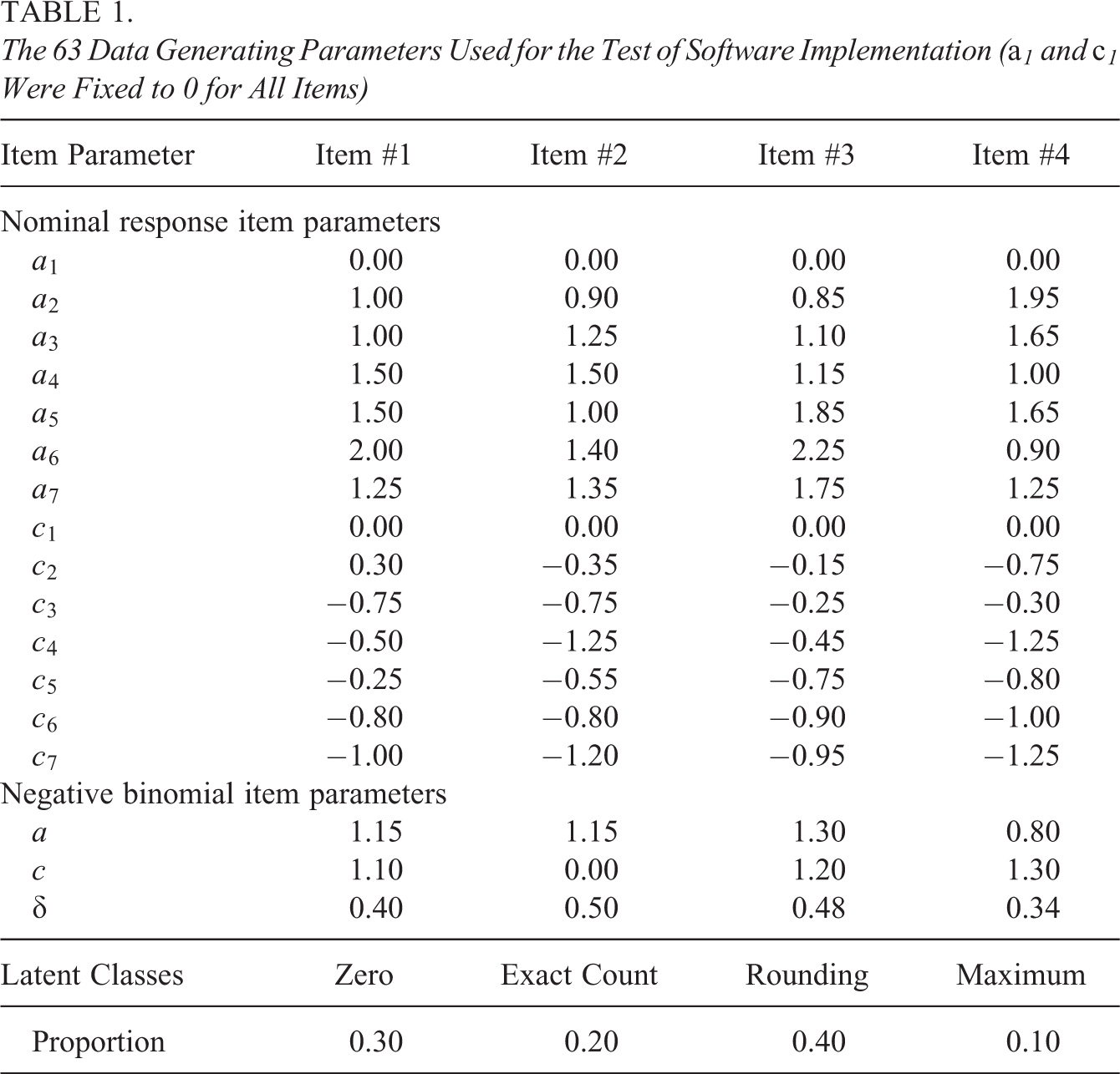
To test the software implementation, we simulated 10,000 responses to four hypothetical count items with a 0 to 30 response scale. First, each of 10,000 observations was assigned to one of the four latent classes. Then, depending on the latent class membership, item response data were generated: For members of the zero and maximum classes, response patterns of
The 63 Data Generating Parameters Used for the Test of Software Implementation (a1 and c1 Were Fixed to 0 for All Items)
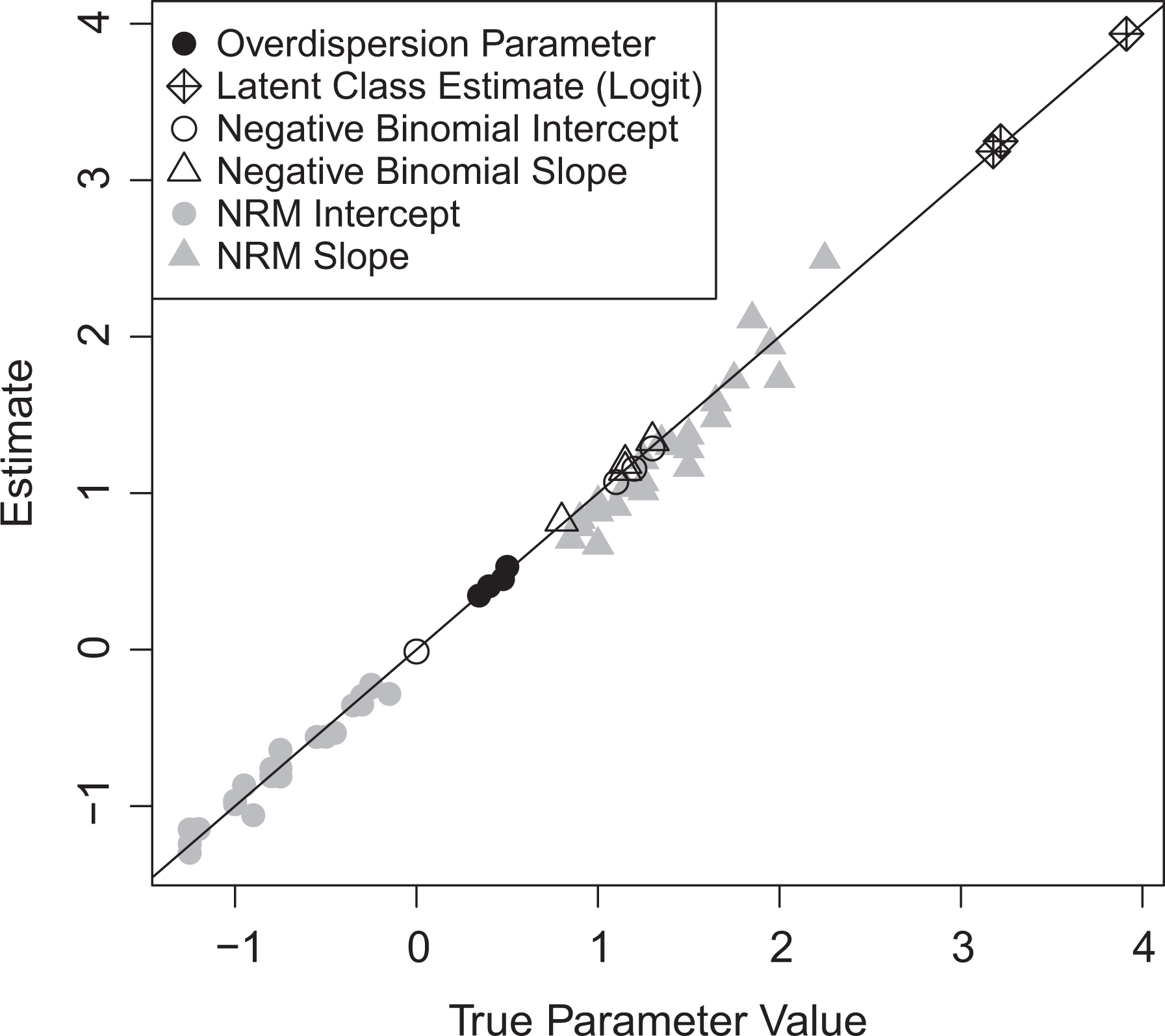
Parameter estimates from the latent class item response theory model (y-axis) relative to the true/data generating parameters (x-axis).
Empirical Analysis of the BRFSS Scale
The analytic sample consisted of 9,042 individuals who responded to a set of four count items from the 2014 version of the BRFSS. The 4 items form a subscale measuring emotional health status, with each item response reported on a 0- to 30-day scale. For the pain, depression, and anxiety items, an increasing number of days suggest worse health; for the energy item, an increasing number of days suggest better health. To maintain consistency of scale direction, the energy item was reverse coded. The names “pain,” “depressed,” “anxious,” and (reversed) “energy” are used to refer to each of the items.
When fit to empirical data, the latent class IRT model converged after 472 iterations, requiring approximately 16.5 hr. Estimates of the proportions of individuals belonging to each of the four latent classes are in the last row of Table 2. Nearly one third of respondents in the sample either (a) treated the items as multiple-choice questions instead of open-ended counts or (b) rounded their answers to the nearest multiple of 5. Only about half of the respondents used the full range of the open-ended count scale in selecting nonmultiple of 5 counts. While 24% of the sample endorsed 0 for every item, only 16% of respondents were estimated to belong to the zero class; such a decomposition indicates that someone endorsing zero for all 4 items has approximately 67% probability of belonging to the zero class and 33% probability of belonging to one of the two graded classes. Of the people who endorsed 30 for every item, 68% were estimated to belong to the maximum class. According to the model, the remaining 45 people with an all-30 response pattern fall along the continuum of the latent variable measured by the scale: poor emotional health.
Parameter Estimates (With Standard Errors) of the Latent Class Item Response Theory Model Fit to the Behavioral Risk Factor Surveillance System Data
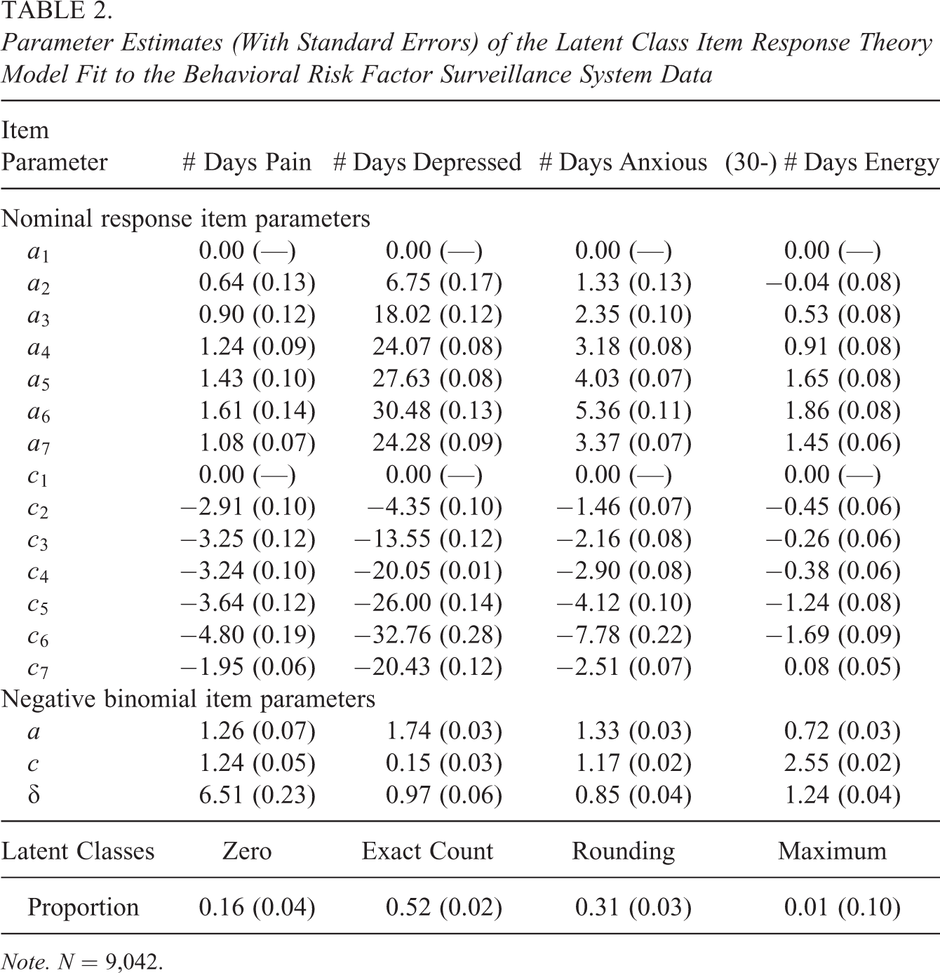
Note. N = 9,042.
IRT parameter estimates can also be found in Table 2. To examine how closely the IRT parameters estimated from the model reproduce the empirical response distributions, we simulated 9,042 responses to the 4 items based on the estimates in Table 2. While comparison of the empirical and model-implied distributions does not allow an analysis of model fit at the response pattern level, comparing the two distributions can help inform whether the IRT models are appropriate for the data. The empirical response distributions for pain, depressed, and anxious—shown in the first three columns of Figure 4—are reproduced fairly well, suggesting that the negative binomial and nominal response IRT models are appropriate model choices for these 3 items; however, the empirical response distribution for (reversed) energy, which is shown in the rightmost column of Figure 4, is not reproduced nearly as well. This is because the negative binomial distribution is unable to account for the increasing number of people reporting counts toward the upper limit of the 0 to 30 count range. Recommendations for alternative model specifications that may better accommodate the energy item are described in the Discussion section.
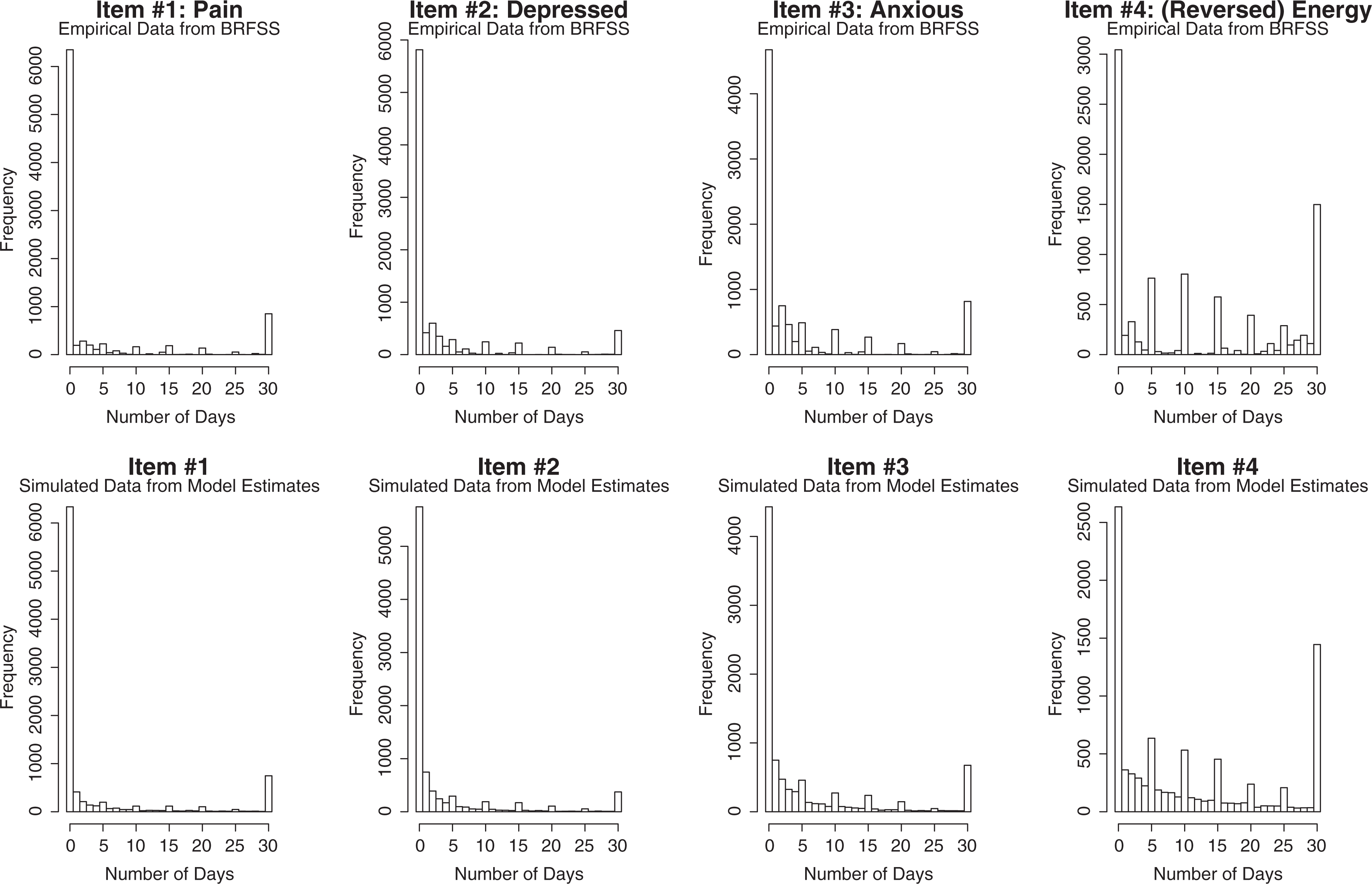
Upper panel: histograms of the four count items on the Behavioral Risk Factor Surveillance System (N = 9,042). Lower panel: histograms of responses simulated from the estimated item response and latent class parameters in Table 2 (N = 9,042).
Interpretation of the Rounding/Selected Response Class
Because the NRM was used to parameterize the response process for members of the rounding/selected response class, the ordering of response categories could be examined empirically. The NRM item parameters show a relatively linear trend: As the number of days category increases, the a parameters tend to increase and c parameters tend to decrease nearly linearly, with the exception of the a and c parameters corresponding to the 30-day category. Anxious and depressed are most discriminating, suggesting that these 2 items are more strongly related to the poor emotional health latent variable than either pain or (reversed) energy. The discriminating ability of these items can also be seen in the trace lines in Figure 5. The trace lines for anxious and depressed tend to function more similarly to each other than either of the other items, likely because the poor emotional health latent variable is really defined by these 2 items, with pain and energy acting as ancillary items.
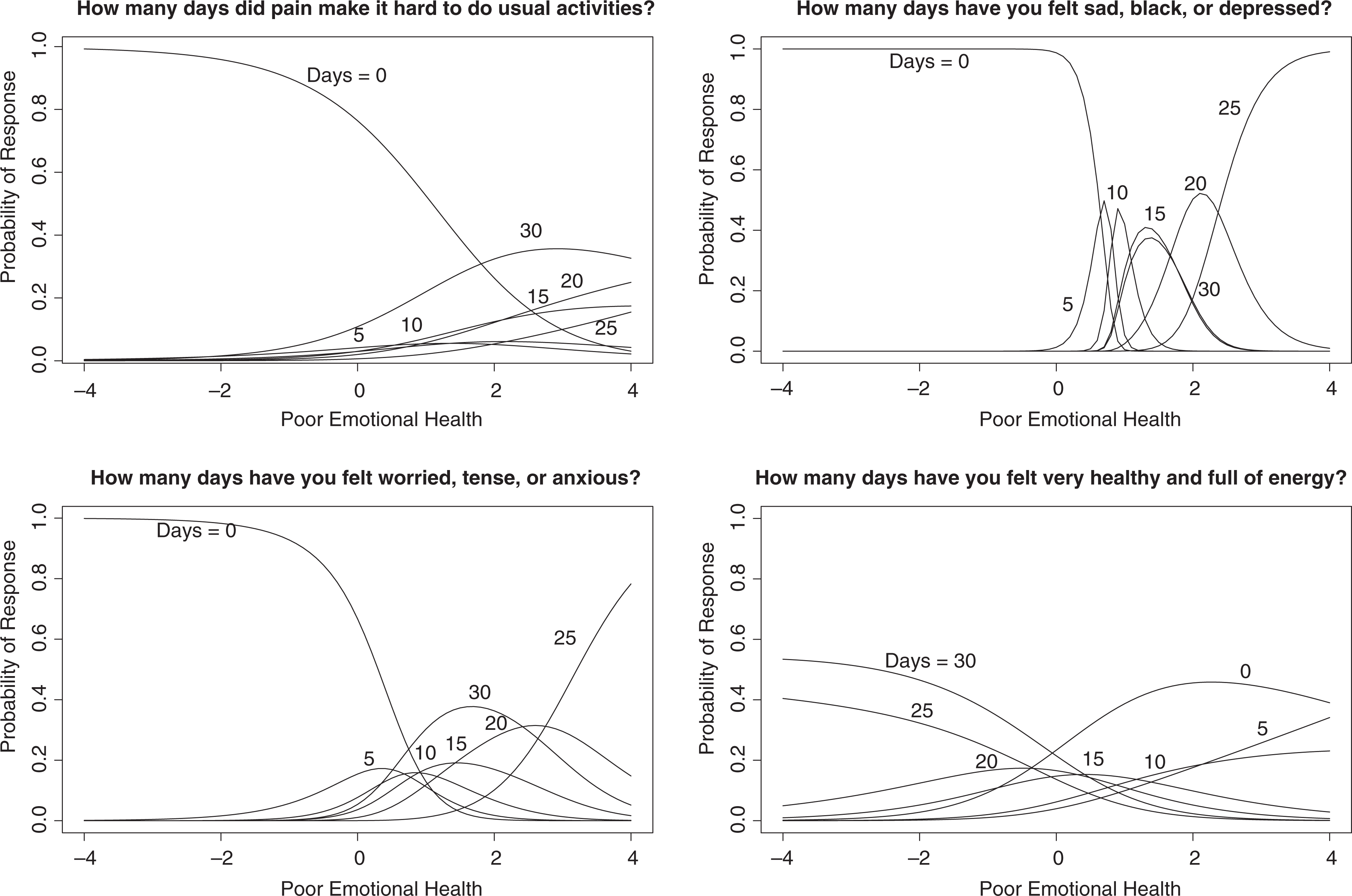
Nominal response trace lines for the rounding/selected response class.
The trace lines in Figure 5 reveal several other item characteristics. First, the 0- and 30-day response categories tend to be associated with the greatest probabilities of endorsement, regardless of someone’s level of the latent variable. This phenomenon is particularly salient in examining the trace lines for the pain and energy items, where at every point along the latent variable, 0 days or 30 days always has a higher probability of endorsement than any of the other response categories. Second, Figure 5 shows that the response categories tend to be in an increasing order for 5 days through 25 days: As one’s level of poor emotional health increases, so does the probability of endorsing a response category that represents a greater number of days (or a lesser number of days for the energy item). The increasing order does not hold for the 30-day response option, however; this is most clearly seen in the trace lines for depressed and anxious, where for people at high levels of poor emotional health, a response of 25 days is actually associated with higher probability of endorsement than a response of 30 days.
The pain, depressed, and anxious items tend to discriminate only among individuals who fall at or above average levels of poor emotional health. This is seen in Figure 5, where for these 3 items, it is not until θ ≥ 0 that the trace lines cross. The relatively flat trace lines for the energy item suggest that this item is only weakly related to the latent variable; people tend to endorse a smaller number of days for this item regardless of their level of poor emotional health. Even for someone at low levels of θ, the probability of endorsing 25 days for energy (or equivalently, 5 days for the reverse-coded energy item) is greater than 0.3. For someone who is at the average level of poor emotional health, there is near-equal probability of endorsing 0 days or 30 days for the energy item. Compared to the other 3 items, the endorsement of lower counts is common for the energy item.
Interpretation of the Exact Count Class
The negative binomial item parameter estimates for the exact count class are also shown in Table 2. The item discrimination for a count item can be interpreted as the log expected change in the number of days associated with a 1 standard deviation (SD) increase in poor emotional health; this value can then be exponentiated to be placed on a more interpretable scale. For a 1 SD increase in poor emotional health, one expects an additional 3.53 days for pain, 5.70 days for depressed, and 3.78 days for anxious; one expects 2.05 fewer days for energy. The c parameter, which is the item intercept, is interpreted as the log expected number of days of a particular symptom for someone who is at the average level of poor emotional health. For someone who is at the average level of poor emotional health, one expects 3.46 days for the pain item, 1.16 days for the depressed item, 3.22 days for the anxious item, and 17.19 days for the energy item (or equivalently, 12.81 days for the reversed energy item).
In fitting a count IRT model to item response data, there are multiple ways to graphically display the item parameters. One option is to plot the trace lines associated with each count IRT model; the negative binomial trace lines for these four count items are shown in the upper two rows of Figure 6. Within a particular plot, each curve corresponds to 1 of the 31 possible open-ended counts, where increasing levels of poor emotional health indicate greater probabilities of endorsing higher counts. Similar to the NRM trace lines, flatter trace lines suggest a weaker relationship between the item and the latent variable, and the location of the trace lines indicates where on the latent variable continuum the item is most discriminating. One can choose a level of the latent variable and find the endorsement probability that corresponds to each of the 31 counts. For the pain item, for example, someone with θ = 0 has roughly a .60 probability of endorsing 0 days, a .1 probability of endorsing 1 day, a .05 probability of endorsing 2 days, and a near-zero probability of endorsing any of the counts greater than 3 days.
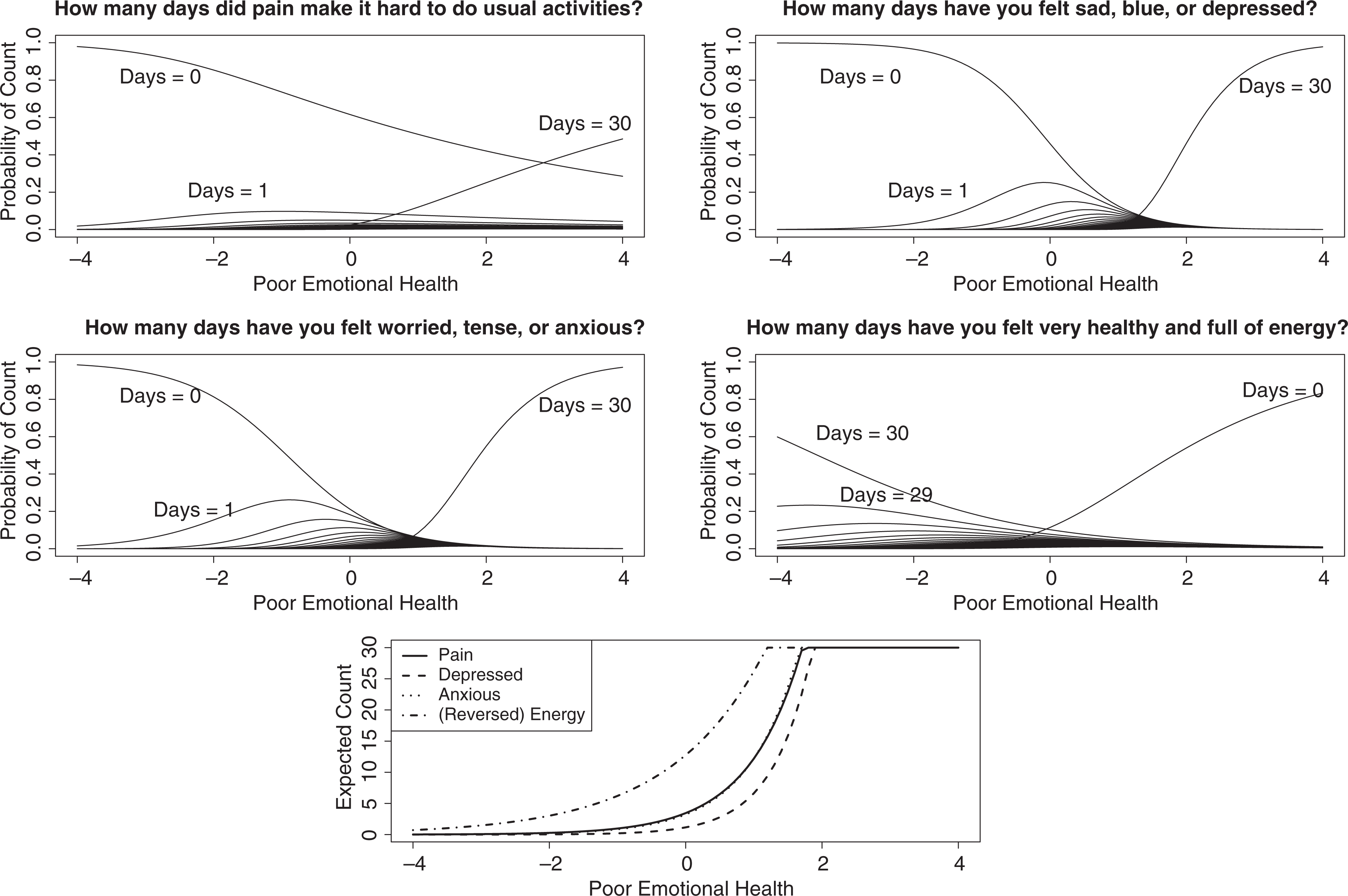
First two rows: negative binomial trace lines describing probability of count endorsement for members of the exact count class. Last row: expected endorsed count as a function of the latent variable for members of the exact count class.
Perhaps a more intuitive approach to visualizing the relationship between the latent variable and the item responses is to plot the expected counts for each item as a function of the latent variable. Such a plot is shown in the lowermost panel of Figure 6. The low discriminating power of the energy item compared to the depressed and anxious items is shown with its flatter slope. The relatively high expected counts for (reversed) energy—even for people with low levels of poor emotional health—is also shown in Figure 6. For someone who is 2 SDs below average on poor emotional health, the expected number of days for pain, depressed, and anxious is approximately 0; for someone at this same level of poor emotional health, the expected number of days for (reversed) energy is 3.
Overall, both pain and energy do a poor job of separating individuals on the latent variable. As was the case for the rounding/selected response class, the 0- and 30-day response options dominate the trace line plots: Across all levels of poor emotional health, these are almost always the response categories with the highest probabilities of endorsement. Figure 6 also suggests that lower counts are more easily endorsed for the energy item, even for individuals at low levels of the latent variable. For example, someone at low levels of poor emotional health has only a modeled 40% to 60% probability of reporting 30 days for the energy item (or equivalently, 0 days for the reverse–coded energy item); for the other 3 items, however, individuals at low levels of poor emotional health have a nearly 100% probability of endorsing the 0-days response option. One explanation is that the energy item is not as strongly related to poor emotional health as the other 3 items. Alternatively, it may just be that the anxious and depressed items are so strongly related to each other that they define the construct that is being measured by the scale, making the other 2 items appear less relevant.
Scale Scores
According to the latent class IRT model, scale scores depend not only on response patterns but also on latent class membership, and one of the complexities involved in scoring is the uncertainty of latent class membership. Because latent class membership is not known a priori, in most cases, it is not possible to directly classify individuals. For many response patterns, there exist two possible class memberships and consequently two plausible scale scores.
Only members of the exact count and rounding/selected response classes fall along the latent variable continuum—this means that only approximately 83% of the population, or 7,498 of the 9,042 people in the sample, should receive scores that are estimates of θ values. To account for the 16% and 1% of the population belonging to the zero and maximum classes, respectively, 1,451 all-0 response patterns and 93 all-30 response patterns were removed, resulting in a scoring sample of 7,498 respondents. Removing a proportion of the all-0 and all-30 response patterns yields score distributions that represent those that would be observed in the population of people belonging to one of the two graded classes. Because it is not possible to identify the specific individuals belonging to the zero and maximum classes, scores are discussed only at the population level and not at the individual level.
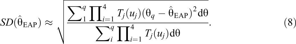
For a given response pattern

where
For individuals known to be members of the exact count class (i.e., their response patterns include at least one count that is not a multiple of 5), a single scale score was computed using the estimated negative binomial trace lines for
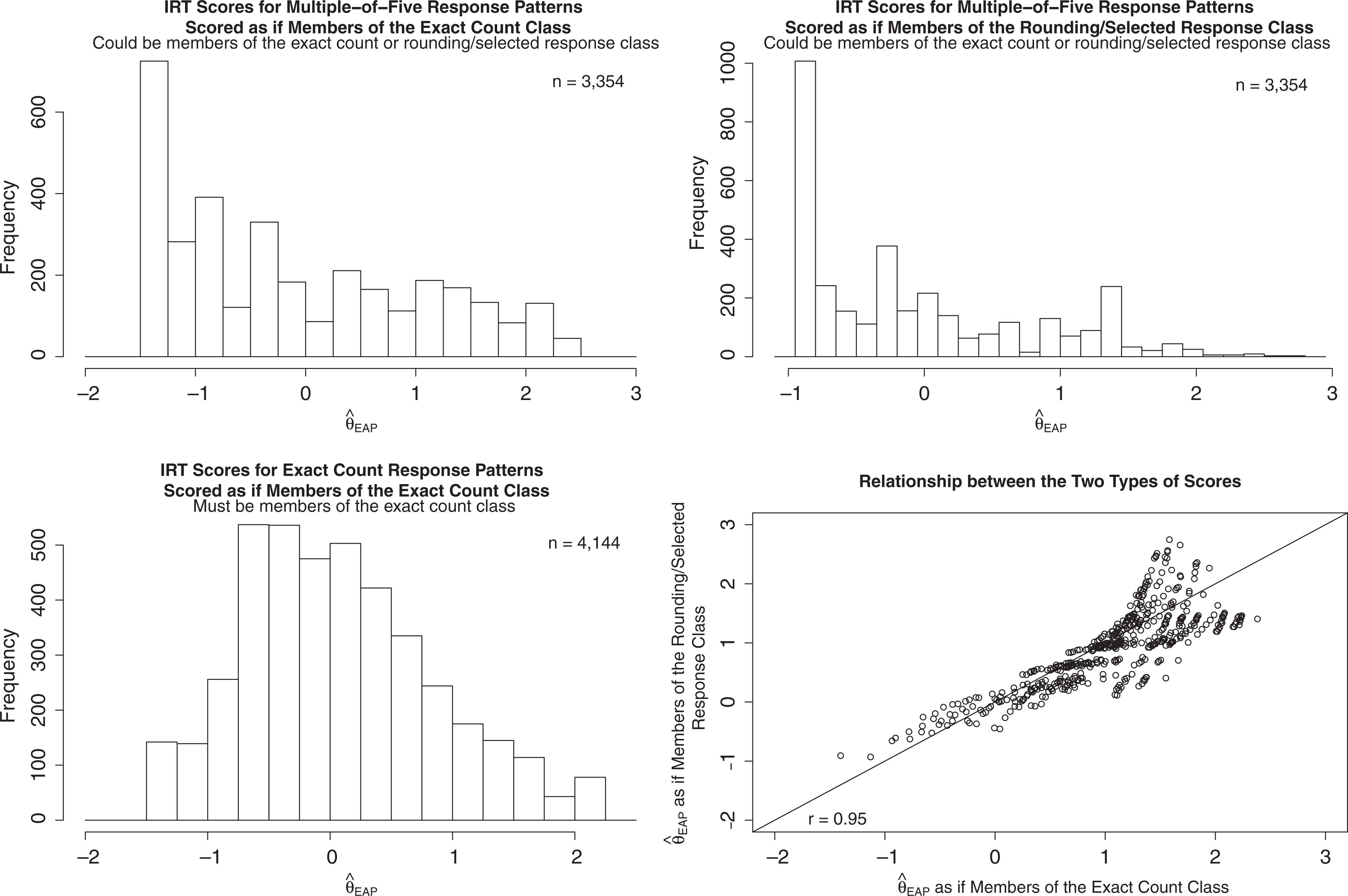
Item response theory scale scores (response pattern expected a posteriori) for members of the exact count and rounding/selected response classes. Upper left: scale scores for multiple of 5 response patterns scored according to the negative binomial trace lines. Upper right: scale scores for multiple of 5 response patterns scored according to the nominal response model trace lines. Lower left: scale scores for nonmultiple of 5 response patterns scored according to the negative binomial trace lines. Lower right: scatterplot showing the relationship between two types of scoring methods for multiple of 5 response patterns.
The lower left panel of Figure 7 shows the scale scores for individuals who must belong to the exact count class. Scale scores range from
Expected Scale Scores and Posterior Standard Deviations Associated With Different Response Patterns: Comparison of the Exact Count and Rounding/Selected Response Classes
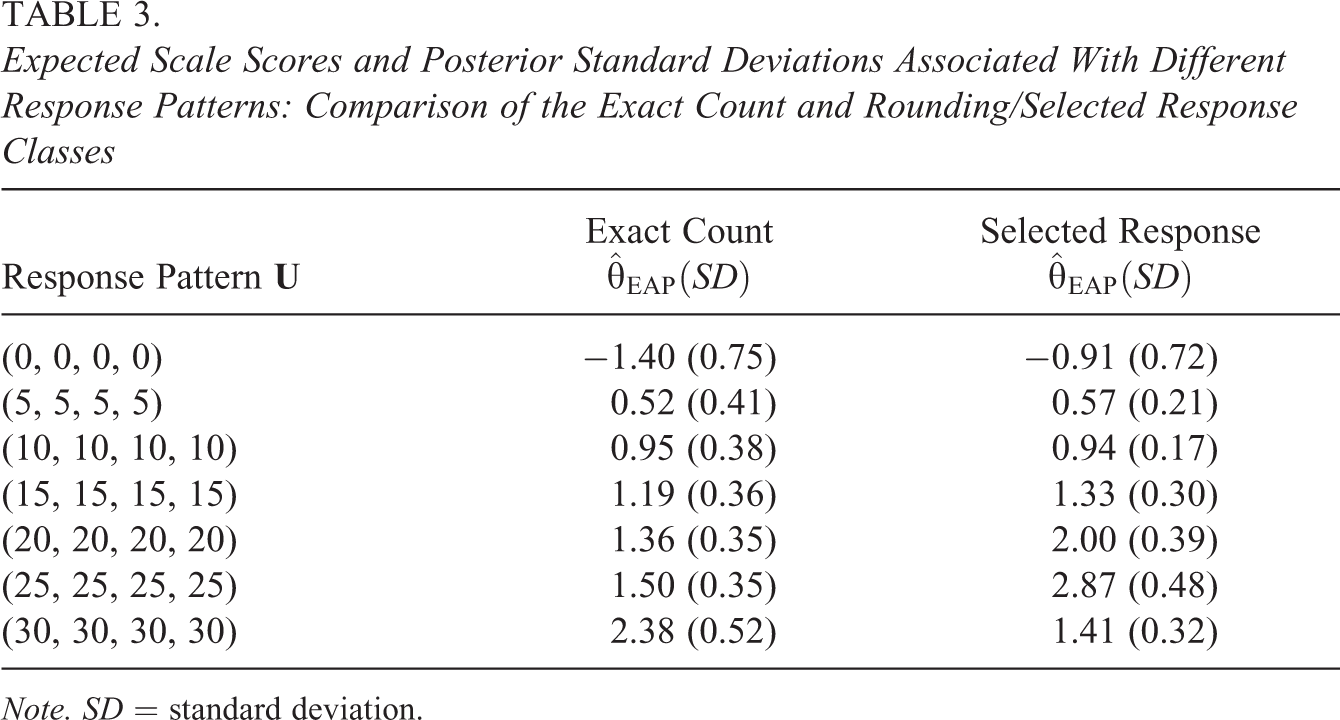
Note. SD = standard deviation.
A researcher planning to use these scale scores in secondary statistical analyses may be interested in the correlation between the two types of scores: Does it matter which type of score is computed for people who could belong to either the exact or rounding/selected response class? The correlation between the two sets of scores is 0.95, with a scatterplot shown in the lower right panel of Figure 7. The scatterplot reveals a funnel-shaped relationship, in which scores are not as highly correlated at the extreme positive end of the latent variable. Table 3 further highlights this trend. The scale score estimates that correspond to response patterns with higher counts, such as
Posterior SDs are plotted in Figure 8. As tends to be true of IRT scores, the posterior SDs are larger at the extreme ends of the latent variable and smaller near values of the latent variable where the items are most discriminating. It is worth noting that the posterior SDs for the exact count class are almost never smaller than those for the rounding/selected response class; they are only lower when scale scores drop below average
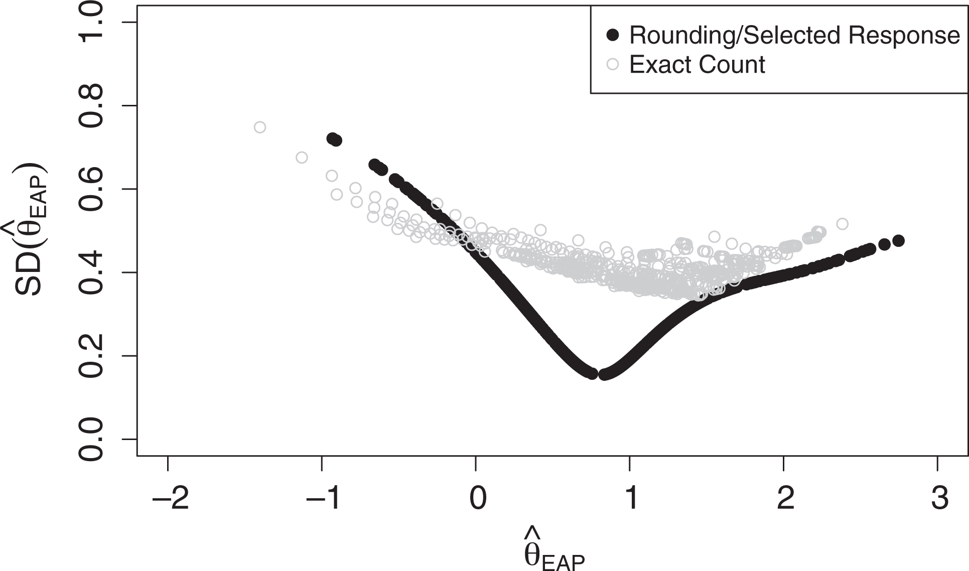
Posterior standard deviations (SDs) as a function of scale scores for the exact count and rounding/selected response classes. The x-axis displays the scale scores observed in the sample; the y-axis shows the posterior standard deviation associated with each of those scale scores.
Discussion
The goal of this research was to develop a latent class IRT model that could account for zero inflation, maximum inflation, and heaping in multivariate open-ended count item response data. Results of the empirical analysis suggest that a latent class IRT model that uses a negative binomial IRT model for the count process, a nominal response IRT model for heaping at preferred digits, and two degenerate IRT models for the zero and maximum classes may be a good approximation for the underlying response process that produces the observed count distributions. The results provide evidence that this modeling approach is useful in analyzing data from scales with multiple open-ended count items—in particular, the four count items from the BRFSS.
The results reveal a peculiarity in the way some people may respond to specific types of open-ended count items on questionnaires, and this peculiarity may have implications for scale development. When retrospectively responding to open-ended count items, a sizable proportion of individuals may not treat the item as an open-ended count but instead may treat it as a selected response item with a smaller number of response categories. While this phenomenon may not be characteristic of all types of count data, it is present within this subscale of the BRFSS. Further, within the rounding/selected response latent class, the seven response categories are not in an increasing order with respect to the latent variable. Specifically, the ordering of response categories suggests that people with the highest levels of poor emotional health are more likely to endorse 25 days than 30 days. Within the rounding/selected response class, someone who endorses 30 days may really mean some large quantity of days (i.e., more than 15). Choosing 30 days with this meaning does not require the respondent to engage in any type of count process. On the other hand, because selecting 25 days reflects the use of some type of count process and not just choosing the maximum response as a shortcut, someone who endorses 25 days likely really means a number around 25 days. This finding is counterintuitive to the inherent ordering of counts that one may expect in designing scales with open-ended count items, and it has implications for researchers who wish to draw conclusions about an individual’s level of poor emotional health from a response pattern that include counts: Higher counts may not always indicate higher levels of the latent variable.
The results also suggest that it is important to account for population heterogeneity in item response data, not only in considering differences in response style but also in recognizing that the scale may not be measuring the same latent variable for all individuals. Specifically, the IRT analyses of the four count items on the BRFSS suggest that 16% of respondents belong to a zero class and 1% of respondents belong to a maximum class. These respondents may be at some floor or ceiling level of the latent variable or, in some sense, not at any value of the latent variable θ at all. For example, someone in the maximum class may fall at such severe levels of poor emotional health that this particular scale should not be used to assess that person—perhaps a different scale that provides more nuanced measurement at the extreme levels of the latent variable should be used instead. Further assessment of people who may belong to the zero or maximum classes is a logical next step. Another reason someone may be a member of the zero or maximum class is that the items may not be relevant to the respondent. Wall et al. (2015) and Finkelman et al. (2011) describe the unipolar nature of many clinical traits, such that a substantial proportion of the sample does not exhibit any of the symptoms or behaviors that are referenced in the items. In describing her zero-inflated Poisson IRT model, L. Wang (2010) explains a similar phenomenon that is commonly observed on questionnaires about substance use, in which many people report zero units of alcohol, cigarettes, and marijuana because they abstain from substance use and the items are not applicable. While the analog to emotional health symptoms is not as intuitive, it is possible that some respondents are so low on psychopathology that they view the items as irrelevant. These individuals who belong to the zero class may be viewed similarly to substance use abstainers. Whatever the reason, ignoring the zero and maximum classes may lead to a biased representation of the latent variable in the population.
Recommendations
The model developed as part of this research is computationally complex. Not only does parameter estimation require several hours of computing time, but to our knowledge, user-friendly software that can implement these types of latent class IRT models is limited or perhaps nonexistent. At minimum, researchers need to directly specify the model log likelihood and use an optimizer such as R’s nlm; more complicated models—for example, those designed for scales with a larger number of items—may require more sophisticated programming knowledge. Researchers can obviate such complex modeling techniques by not including items that elicit a retrospective count response on their scales and questionnaires. Alternative methods of framing the question can simplify item-level analyses.
Perhaps the simplest strategy to avoid eliciting open-ended count responses is to bin the response options before administering the questionnaire. Binning eliminates the issue of individual differences in response style, such that the exact count and rounding/selected response classes are no longer needed. It may reduce recall error. Framing the question with binned counts is less taxing on the respondent’s memory than asking for a cumulative raw frequency. While binning may eliminate some of the issues associated with retrospectively reported open-ended count data, it can introduce other statistical modeling challenges (McGinley, Curran, & Hedeker, 2015). If one wishes to preserve raw frequencies, a more reliable approach may be to use a daily diary response format instead of retrospective counts. The daily counts could then be tallied to obtain a more accurate total frequency. One advantage of this approach is that because respondents are not retrospectively reporting a cumulative frequency, heaping is much less likely to be present in the observed item response data. Without heaping, a rounding/selected response class is no longer needed to account for digit preference, and a simple count IRT model may be sufficient. This reduction in parameters would greatly reduce estimation time as well as the complexities involved in scoring individuals when class membership is unknown. Because the results suggest that items eliciting raw count responses can substantially reduce the SDs of scale scores, the daily diary approach may be preferable to binning the counts, as the true count nature of the data is preserved and more information is available in each item response. Future research could investigate this topic.
Limitations
One of the major limitations of using open-ended count IRT models is the difficulty of assessing absolute model fit. As the number of count items increases, the number of possible response patterns becomes unmanageably large, producing multiway contingency tables with extreme sparseness. Such sparseness creates challenges in the development of goodness-of-fit statistics that compare observed and expected response pattern frequencies. Currently, examination of fit is limited to measures of relative model fit that can be computed from the model log likelihood such as the Akaike information criterion (AIC) and Bayesian information criterion (BIC).
The negative binomial IRT model assumes that the observed counts are unbounded. For most of the count items, this IRT models serve as reasonable approximations for the empirical response distributions—very high counts are rarely observed in the data, and most of the 30s are manifestations of a rounding or selected response process, not a count process. However, an IRT model that uses a bounded conditional count response distribution, such as a beta-binomial distribution, is likely more appropriate for 30-day recall items in which observations toward the upper limit are frequent. Future extensions of this work could include beta-binomial IRT models for the exact count class to accommodate bounded count responses.
Conclusions
The goal of this research was to develop an IRT model that could address some of the challenges that commonly arise in analyzing multivariate count data from questionnaires. The proposed model integrates elements from three different methodological approaches rooted in psychometrics and biostatistics: IRT models for zero-inflated count data, latent variable models for heaping and response style, and latent class IRT. While not without limitations, the latent class IRT model is able to address many of the issues involved in analyzing the multivariate open-ended count items that are becoming more common in clinical assessment, and we believe that they show promise of wider applicability in the field of psychological measurement.
Footnotes
Declaration of Conflicting Interests
The author(s) declared no potential conflicts of interest with respect to the research, authorship, and/or publication of this article.
Funding
The author(s) received no financial support for the research, authorship, and/or publication of this article.