
Abstract
Nondichotomous response models have been of greater interest in recent years due to the increasing use of different scoring methods and various performance measures. As an important alternative to dichotomous scoring, the use of continuous response formats has been found in the literature. To assess finer-grained skills or attributes and to extract information with diagnostic value from continuous response data, a multidimensional skills diagnosis model for continuous response is proposed. An expectation-maximization implementation of marginal maximum likelihood estimation is developed to estimate its parameters. The viability of the proposed model is shown via a simulation study and a real data example. The proposed model is also shown to provide a substantial improvement in attribute classification when compared to a model based on dichotomized continuous responses.
1. Introduction
Due to the increasing use of different scoring methods and various performance measures, interest in nondichotomous response models has grown in the last several decades. Recent research, some of which will be discussed in this article, has addressed polytomous item response models in the context of both traditional item response theory (IRT) and cognitive diagnosis models (CDMs). However, far less effort, particularly for CDMs, has been devoted to modeling continuous response, which has been found in at least the following three areas and will be discussed in turn: (1) providing a level of endorsement by marking a continuum, (2) “probability testing,” and (3) the use of latency data.
The purpose of this article is to present an adaptation of the deterministic inputs, noisy “AND” gate (DINA; Haertel, 1989; Junker & Sijtsma, 2001) model that handles continuous response. Although this model is presented as a general framework that may be used or modified for other types of continuous response measures, we will discuss it in the context of analyzing latency data. In many cases, latency data are readily available alongside response accuracy data, and proper analysis may yield additional diagnostic insights. The sections that follow will discuss the aforementioned three types of continuous response data, with a brief overview of some of the models that have been developed to analyze such data. Next, a review of CDMs will be presented, from which the continuous response version of the DINA model and its estimation procedures will be developed. Finally, a simulation study and a real data example, followed by a discussion, will demonstrate the viability of the proposed model.
1.1. Continuous Response as a Measure
In some tasks that appear on personality and attitude assessments, respondents are asked to report their level of endorsement with various statements by placing a mark somewhere on a line segment, the ends of which represent the lack of endorsement and complete endorsement. The distance from one of the ends of the segment to the mark can be used as the measure. Noel and Dauvier (2007) have developed an IRT model to handle such a response. Their model is predicated on the notion that such a response format is essentially an infinite-category Likert-type scale. They discuss the idea that more Likert categories are preferable to fewer categories because they provide finer-grained measurement but that the downside of additional categories is that they require the estimation of additional parameters. In general, a Likert-type scale of a large number of graded options is usually considered to be continuous (e.g., Samejima, 1973; Thissen, Steinberg, Pyszczynski, & Greenberg, 1983). Noel and Dauvier (2007) postulate that the β distribution has properties that make it an appropriate choice for the “interpolation response mechanism” that this type of response measure represents (p. 49). An extension of this model by Noel (2014) can handle responses that are of an unfolding nature. This scoring method can also be used in other situations in which a Likert-type scale would be appropriate, such as pain intensity assessment (e.g., Morin & Bushnell, 1998).
Another source of continuous response that is similar to the response format in the previous paragraph comes from probability testing. Using multiple-choice questions, examinees are asked to report the probability that each option is the correct answer rather than actually choosing one of the alternatives. These probabilities are considered to reveal partial knowledge (de Finetti, 1965). In some situations, this method is simplified. In one such simplification, for example, the examinees are asked to express their confidence only for the most correct option, usually by using a Likert-type scale. Such a scoring method is referred to as “confidence marking” and was, to our knowledge, first suggested and applied by Dressel and Schmidt (1953, as cited in Ben-Simon, Budescu, & Nevo, 1997). The merits of both methods over dichotomous scoring are discussed by Ben-Simon, Budescu, and Nevo (1997).
Perhaps one of the most popular sources of continuous responses is response time, thanks in large part to the rapid expansion of computer-based testing in recent years. In computer-based testing, response times have been used to detect aberrant responses (van der Linden & Guo, 2008; van der Linden & van Krimpen-Stoop, 2003), improve item selection in computerized adaptive testing (Fan, Wang, Chang, & Douglas, 2012; Sie, Finkelman, Riley, & Smits, 2015; van der Linden, 2008), control differential speededness in computerized adaptive testing (van der Linden, 2009; van der Linden, Scrams, & Schnipke, 1999; van der Linden & Xiong, 2013), and control differential speededness in multistage testing (van der Linden, Breithaupt, Chuah, & Zhang, 2007). Response times have also been used to improve parameter estimates (Meng, Tao, & Chang, 2015; Ranger & Kuhn, 2012), ability estimates (Ferrando & Lorenzo-Seva, 2007 Meng et al., 2015; Meng, Tao, & Shi, 2014), and ability classifications (Sie et al., 2015) under certain conditions. Uncertainty on personality assessments can also be assessed using response time (e.g., Ferrando & Lorenzo-Seva, 2007; Meng et al., 2014). Finally, the fact that most power tests are administered under time constraints necessitates the study of latency in addition to correctness (e.g., Hambleton & Swaminathan, 1985; van der Linden & Hambleton, 1997).
To address the growing prevalence and importance of continuous measures, a number of continuous response models have been proposed for the IRT framework. Possibly the earliest development of a continuous response model in IRT is by Samejima (1973), who showed that the “limiting” (p. 204) case of the graded response model (Samejima, 1969) can be viewed as a continuous response model. Such a response model can be used either in the unidimensional (Samejima, 1973), for which Wang and Zeng (1998) have developed an expectation-maximization (EM) estimation algorithm, or in the multidimensional case (Samejima, 1974).
More recently, van der Linden (2007) has provided a model framework for studying response time and response accuracy simultaneously. In the first level of his hierarchical model, separate item response models for response time and response accuracy are specified, each of which arises from a unique latent trait. The second level of the model relates latent traits through a multivariate normal distribution. Van der Maas and Wagenmakers (2005) use response time in a different way. They develop a model in which the scoring rule itself incorporates response time, rather than dealing with response time separately. Total test score is comprised of the sum of the time remaining for each question (i.e., the time limit less the response time) summed over all correct items. Maris and van der Maas (2012) note that such a scoring rule may encourage guessing behavior and propose an adjusted scoring rule that penalizes incorrect responses that are made too quickly.
It is important to note that these models all assume that the underlying latent trait is continuous, as is typical in IRT, with the exception of van der Linden’s (2007) framework, which is less specific in the sense that it can handle any item response model. As such, there is a need for continuous response models in the cognitive diagnosis modeling framework.
1.2. CDMs
In a typical IRT application, the continuous latent trait is usually unidimensional and broadly defined. In contrast, CDMs use a latent, multidimensional, discrete vector as the person-specific variable and are designed to assess finer-grained skills and to extract information with more diagnostic value. The goal of analyzing data with a CDM is generally to determine which of a set of discrete skills examinees have mastered. The set of skills that examinee i possesses is referred to as the attribute pattern, which is an unobservable latent variable represented by a vector of length K, denoted as α
i
. Entries of 1 and 0 indicate the presence or absence of that skill, respectively. Correspondingly, a
The DINA (Haertel, 1989; Junker & Sijtsma, 2001) model is a commonly used and readily interpretable CDM. Its latent response variable is defined such that only examinees who possess all of the skills required to solve a given item are expected to answer correctly; examinees who are missing one or more skills are not differentiated from those who have no skills. Thus, each item partitions examinees into two latent groups, from which the slip (s) and guessing (g) parameters are estimated. The g parameter denotes the probability that an examinee who is missing one or more required skills provides a correct response; similarly, the s parameter denotes the probability that an examinee who possesses all required skills answers the question incorrectly. Occasionally, 1 − s is used rather than s; with 1 − s, the interpretation becomes the probability that examinees who have all required skills answer the question correctly. Additional details for the DINA model can be found in de la Torre (2009b) and de la Torre and Douglas (2004).
Related to the DINA is the deterministic inputs, noisy “OR” gate (DINO; Templen & Henson, 2006) model. DINO items also partition examinees into two groups, but the two groups are defined differently than they are in the DINA model. The model only requires that examinees possess one required skill to provide a correct response; possessing additional skills does not change the probability of responding correctly. Only examinees who possess none of the required attributes are expected to respond incorrectly.
The generalized-DINA (G-DINA; de la Torre, 2011) model relaxes the simplifying constraints in the DINA and DINO models and allows for additional latent groups with intermediate probabilities of success to exist. Rather than partitioning examinees into two latent groups on each item as is done in the DINA and DINO models, the G-DINA partitions examinees into
Although CDMs such as these represent important contributions to the literature, most CDMs can only handle dichotomous, and in a few cases, polytomous data (e.g., de la Torre, 2009a; Ma & de la Torre, 2016). To extract information with diagnostic value from the research settings involving continuous measures, a DINA-like CDM for continuous response will be introduced.
2. The DINA Model for Continuous Response
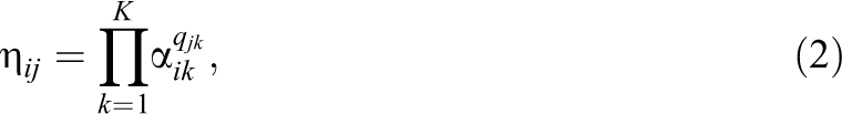
Let Xij denote the response of examinee i to item j, where

where
and
where
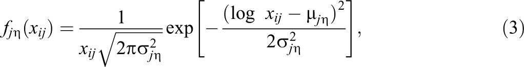
Note that the density given in Equation 3 may be replaced with any probability density function. For applications involving response time, such as those discussed in this article, a lognormal distribution has been shown to be appropriate (van der Linden, 2006). For applications in which the response is bounded (e.g., placing a mark on a line, probability testing, etc.), a distribution with finite support may be desired, such as the 2- or 4-parameter β distribution. Such an adjustment would represent a relatively minor interpretive extension to this model; however, substantial work would need to be done to revise the marginalized maximum likelihood estimation (MMLE; Bock & Aitkin, 1981) and standard error (SE) algorithms that are presented in Appendix A, particularly if the β distribution is desired due to the complexity of its first and second derivatives. To make this adjustment, the following changes would need to be made in addition to adjusting the notation to ensure its appropriateness: The derivatives in Equation 3 would need to be taken based on the distribution being used, and Equations 18, 19, 20, and 21 would need to be updated accordingly. It should also be noted that closed-form estimators may not be available depending on the distribution used. Updating the SE computation would involve changes to Equations 25 and 26. The simpler but more computationally intensive Markov chain Monte Carlo estimation technique could be used as well.
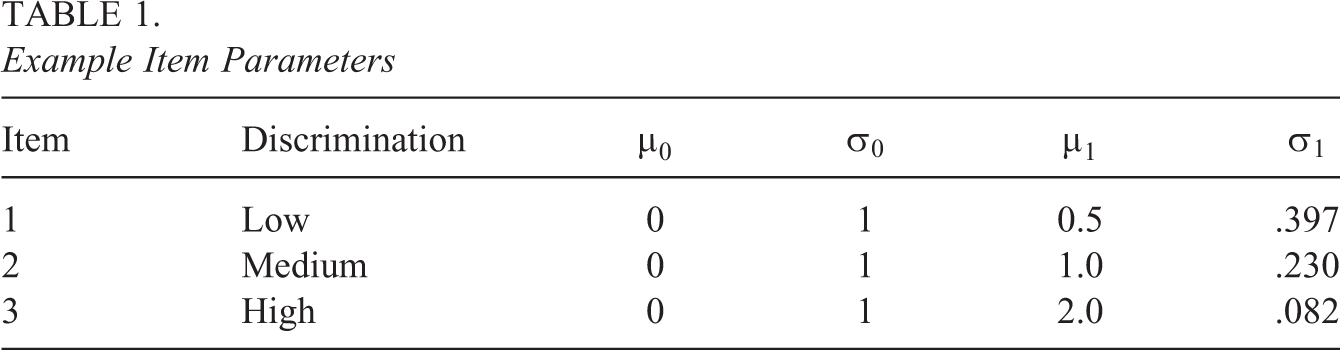
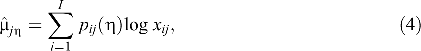
Three items with varying degrees of discrimination are shown in Figure 1. Items 1, 2, and 3 represent items with low, moderate, and high discriminations, respectively. The amount of overlap between the distributions corresponds inversely to the item’s discrimination. An item’s discrimination refers to its ability to differentiate the responses of examinees in
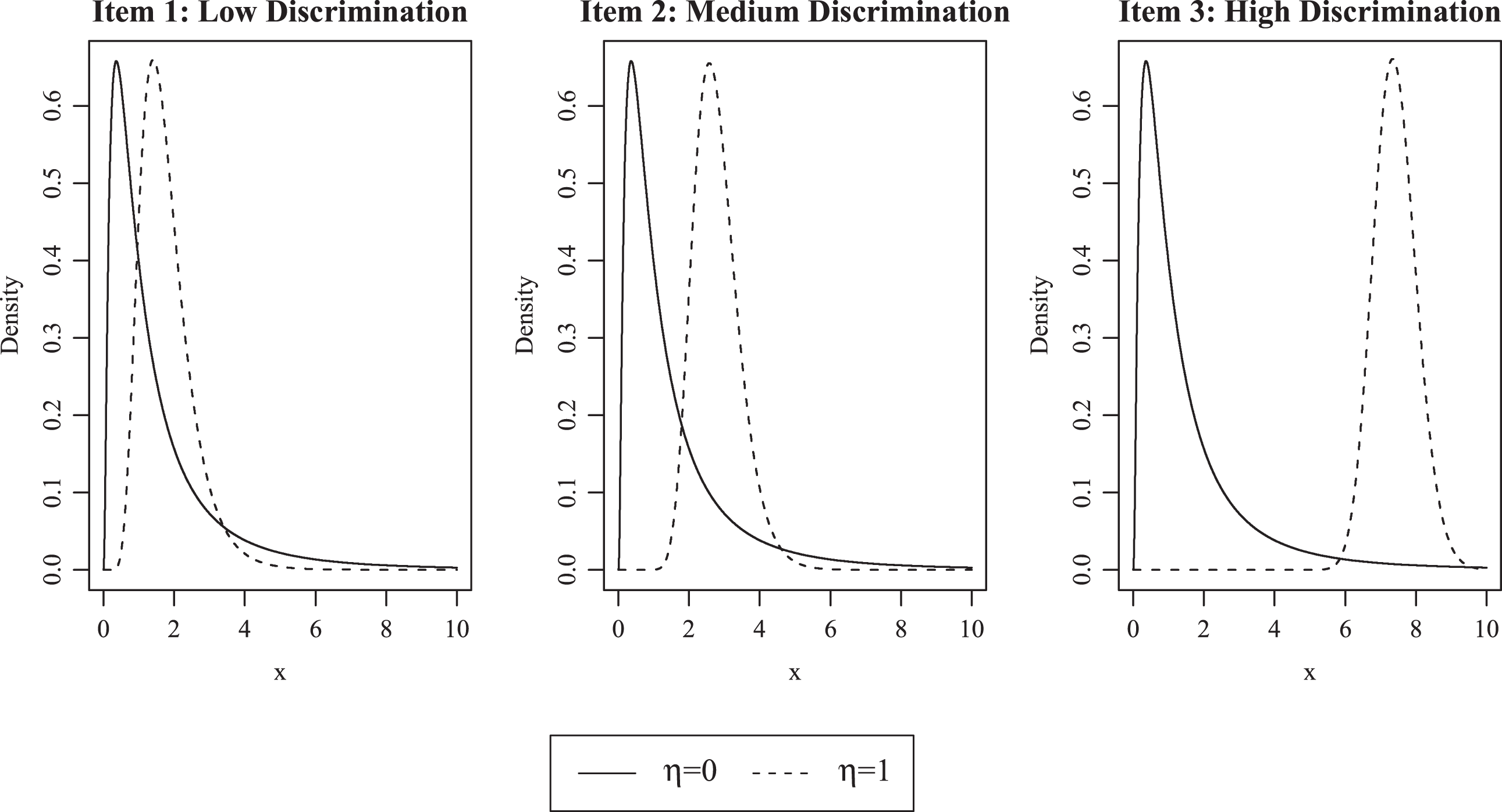
Probability density curves of 3 items with different discriminations.
Example Item Parameters
To measure the discrimination of these items, an index that quantifies the difference between the two distributions is needed. A crude way to accomplish this is to compare the means of the two distributions, as in
3. Estimation
The parameters of the C-DINA model,
and
where
Similarly, the SEs of the parameter estimates of item j can be approximated by the square root of the diagonal elements of
where
For the approximation implemented in this article, Equation 6 involves inversion of a diagonal matrix.
4. Simulation Study
A simulation study was carried out to investigate the viability of the proposed C-DINA model. Specifically, the study was designed to determine how estimation of the C-DINA model parameters and its attribute classification rate are affected by three factors—test length (J), sample size (I), and item discrimination. Additionally, the study examined how the attribute classification accuracy of the C-DINA model compared to that of the DINA model when the continuous response was dichotomized. The code to estimate the model was written in R (R Core Team, 2015).
4.1. Design and Analysis
Two test lengths (J = 15, 30), three sample sizes (I = 500, 1,000, 2,000), and the three discriminations presented in Table 1 were considered. Note that only the parameters for
Simulation Study Q-matrix
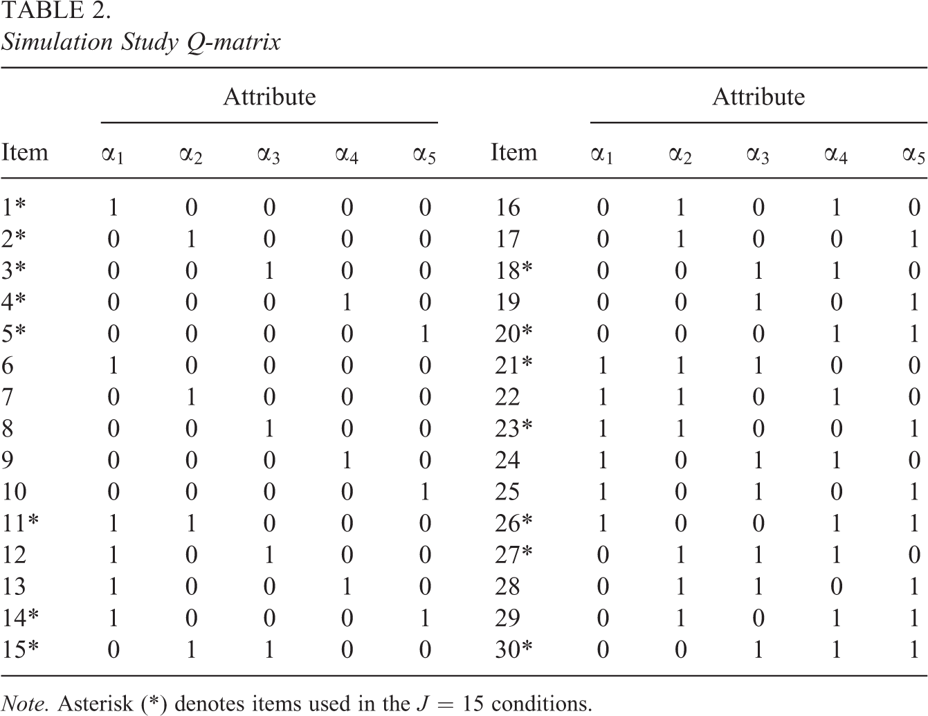
Note. Asterisk (*) denotes items used in the
The quality of the item parameter estimates for a given combination of conditions was summarized by computing the mean bias and variability across the 100 replications. Using the marginal probabilities of the posterior distributions to classify the examinees, classification accuracy was computed at both the attribute and vector levels. For comparison purposes, the generated responses were reduced to dichotomous data and analyzed using the DINA model. The objective of the dichotomization rule was to maximize the separation between the response curve densities of groups
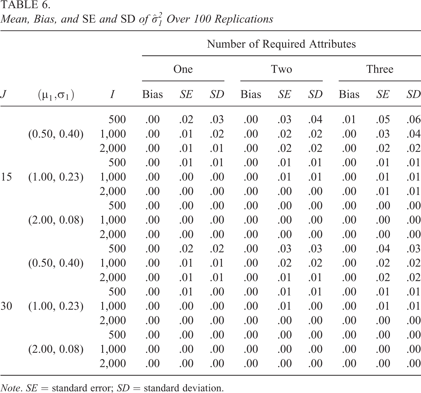
4.2. Results
Tables 3 and 4 summarize the results for the estimates of
Mean, Bias, and SE and SD of
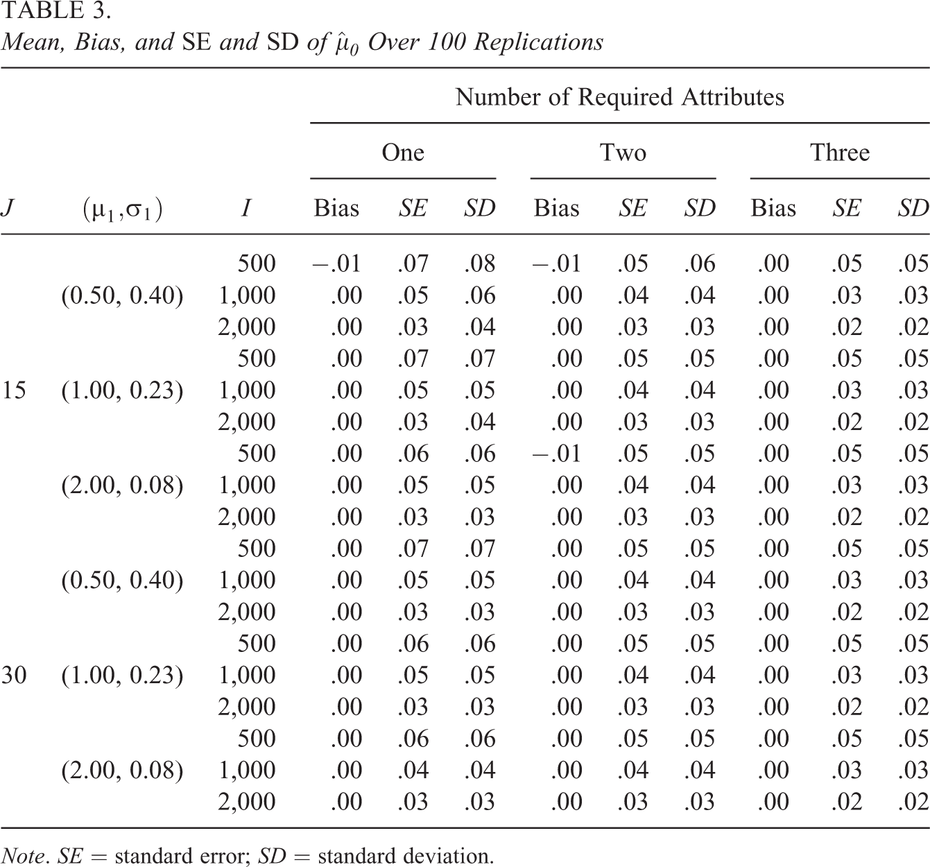
Note. SE = standard error; SD = standard deviation.
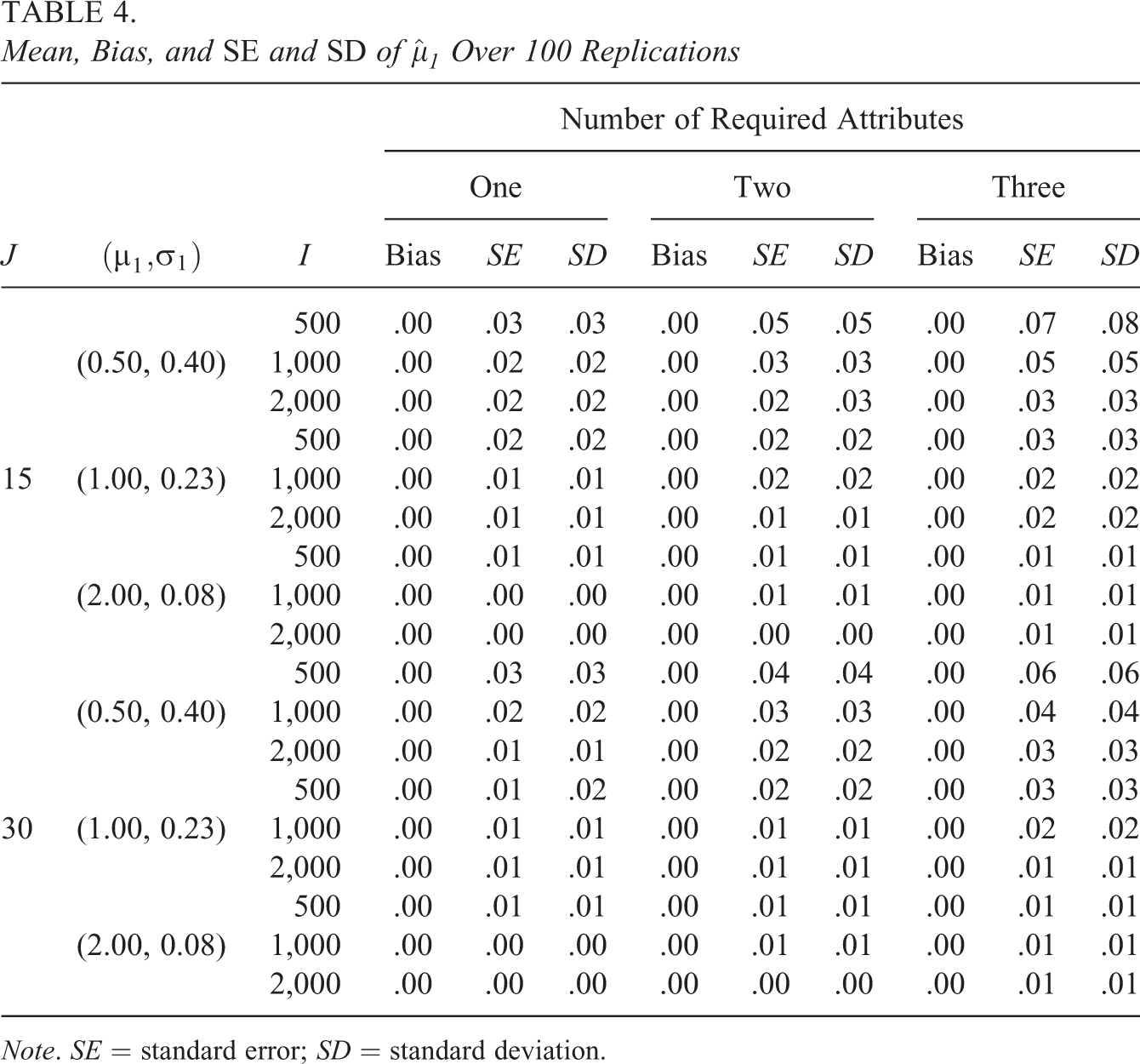
Mean, Bias, and SE and SD of
Note. SE = standard error; SD = standard deviation.
Mean, Bias, and SE and SD of
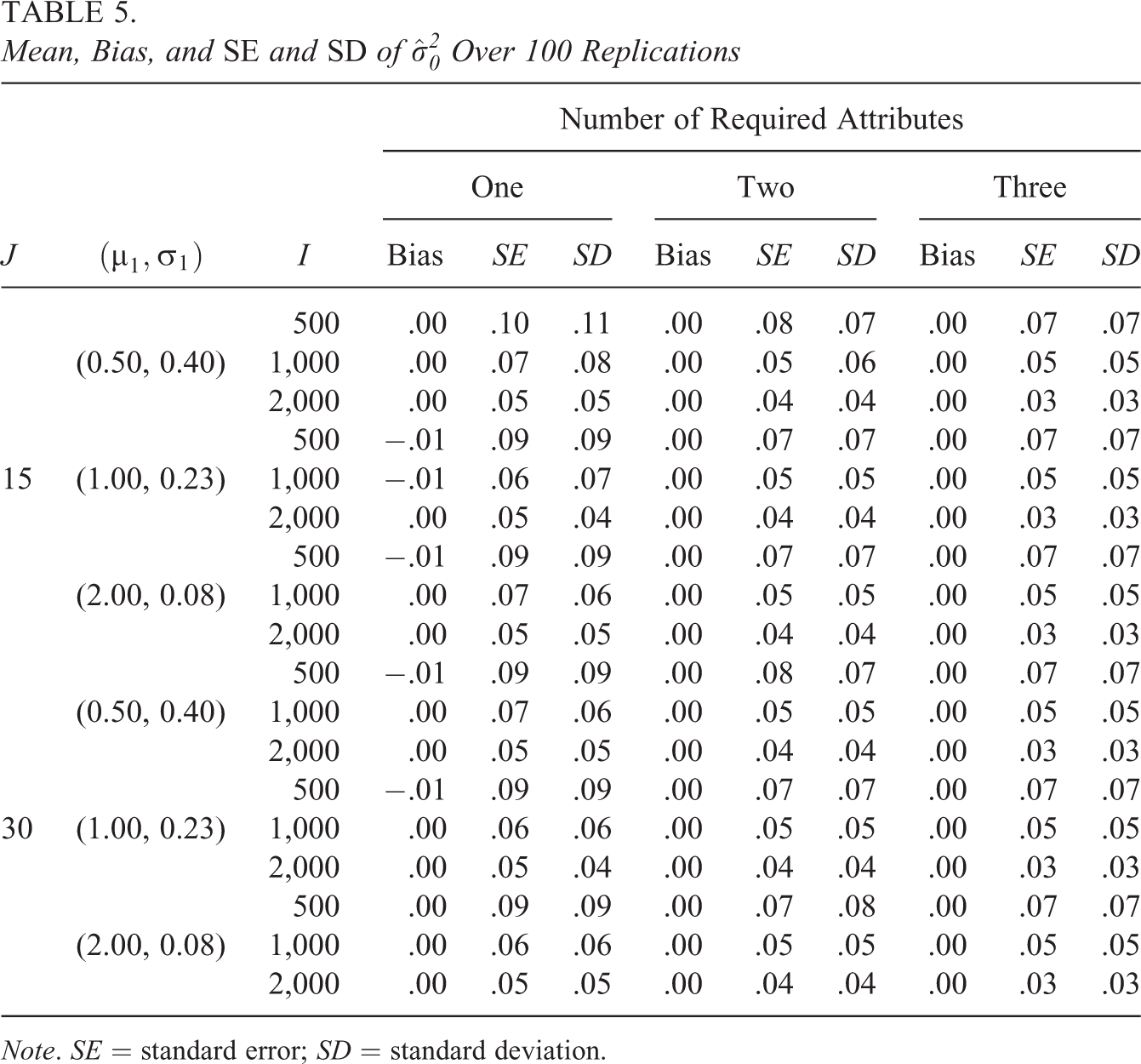
Note. SE = standard error; SD = standard deviation.
Mean, Bias, and SE and SD of
Note. SE = standard error; SD = standard deviation.
Virtually all conditions resulted in unbiased estimates, with just a few conditions resulting in a small negative bias of 0.01. The analytical SEs that were computed using Equation 6 were very close to the corresponding empirical SEs of the estimates. At most, they differed by less than 0.02 but frequently were identical to the second decimal place. Thus, we will discuss variability in general without making a distinction between these two measures. There was also a consistent pattern to the variability with respect to the number of attributes and η. For
Table 3 indicates that variability in
Compared with
Similar to the other parameters, Table 5 indicates that variability for
The results for
Finally, the correct attribute- and vector-wise classification rates are shown in Table 7. In contrast to its effect on parameter estimation, sample size had a minimal (but positive) impact on classification whereas discrimination played a much more prominent role—increasing the separation between the responses of the two groups dramatically increased the correct classification rates for both models. Within a test length, increasing discrimination increased the classification accuracy for both models, but at a slower rate for the C-DINA, meaning that the improvement over the DINA model lessened. Generally, increasing the test length resulted in improved classification, but doing so affected the models differently, resulting in different levels of gain. For example, for the low discrimination condition, increasing the test length improved classifications, but did so to a greater degree for the C-DINA, resulting in an increased gain. For medium and high discrimination conditions, increasing the test length improved accuracy for the DINA model more than for the C-DINA, resulting in slightly lower gains for the longer test. This could be due to the fact that the C-DINA rapidly approached classification accuracy in the mid-to high-90 percentage range as the favorability of the conditions improved. The gain offered by the C-DINA model diminished to less than 2 percentage points at the vector level and less than 1 percentage point for the attribute level when the discrimination was high.
Mean Classification Accuracy Rates for the DINA and C-DINA Models
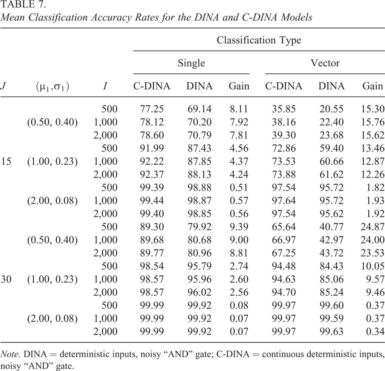
Note. DINA = deterministic inputs, noisy “AND” gate; C-DINA = continuous deterministic inputs, noisy “AND” gate.
In comparison to results obtained using dichotomized data, the classification rates using continuous data were always better. The differences were greatest when the discrimination was low and when considering vector-level classification accuracy. As the items became more discriminating, the differences between the DINA and C-DINA models became negligible.
5. Real Data Example
5.1. Data Description
Van der Maas and Jansen (2003) suggested that examining response times may provide additional insight into the cognitive processes that underlie a test beyond what response accuracy data shows. Siegler (1989) also suggested that response time analyses may be very useful in examining the strategies that examinees use to solve a problem. As such, we applied both the DINA and C-DINA models to a data set of responses and response times of students on balance scale tasks collected and originally analyzed by van der Maas and Jansen (2003).
On the balance scale task, a participant is asked to predict the movement of the scale—tilting to the left, tilting to the right, or balanced. On both arms of the scale, pegs are situated at equal distances from each other and from the fulcrum. On each side of the fulcrum, one or more identical weights are placed on a single peg; the weights placed on each side need not be equal in number nor in distance from the fulcrum. In fact, it is the differences in the numbers and the distances that define the problem type. Participants’ responses to the various types of balance scale items reveal the sets of skills they possess.
The balance scale problems require students to employ increasingly complex skills, which can be viewed as being developmental in nature (Siegler, 1976, 1981). Van der Maas and Jansen (2003) derived the required steps for each item type from the basic model proposed by Siegler (1981). The original data collected by van der Maas and Jansen (2003) consisted of responses from 191 students (147 primary and secondary school and 44 college students) on eight item types, for which the data were complete on seven. To apply the models, we analyzed the responses and response times (in seconds) of the primary and secondary students on four of the seven item types. We removed examinees with ages greater than 16, and those for whom no age was recorded, resulting in a final sample of 146 students.
We began by using all seven item types, of which three were removed. One was removed because of a relationship with age that was opposite to that of the other question types. Two more were removed because they were very easy with proportions correct in excess of 0.9 (van der Maas & Jansen, 2003, p. 156); generally, these item types do not differentiate well between the
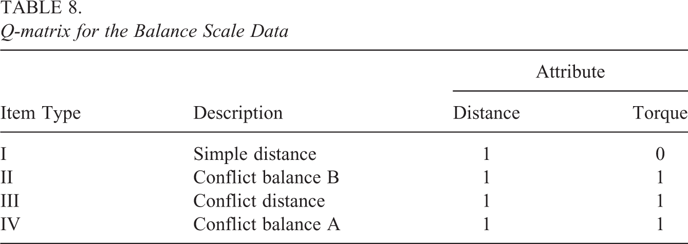
The Q-matrix was constructed based on the following steps required to solve each problem type: (1) comparing the distances at which the weights are placed and (2) applying the torque rule (van der Maas & Jansen, 2003). In the context of CDM, these steps may be interpreted as attributes. Van der Maas and Jansen (2003) hypothesized that the time required to complete a question is directly related to the steps required to solve it correctly. Increasingly, complex items require the application of complex steps beyond the required basic steps and thus require more time to complete. Therefore, the Q-matrix used for response accuracy analyses can also be used response time analyses.
The resulting Q-matrix is presented in Table 8. There were 10 items for each of the four item types for a total of 40 items. Because this application involved developmental attributes, we constrained the possible attribute patterns such that mastery of an attribute implies mastery of all lower level attributes. Thus, in this study, only three such patterns were estimated:
Q-matrix for the Balance Scale Data
Although our primary goal was to analyze response time using the C-DINA model, we began by applying the DINA model to the response accuracy to determine the starting values for the C-DINA EM algorithm. With the DINA classifications, we partitioned the examinees into
5.2. Results
The C-DINA model parameter estimates and the corresponding SEs for these data can be found in Table 9. Instead of presenting the estimates for the 40 items individually, the table lists the mean estimates across the 10 items for each item type. Unlike the normal distribution, the first and second moments of the lognormal distribution are dependent upon both μ and σ parameters. Specifically,
C-DINA Model Parameter Estimates for the Balance Scale Data
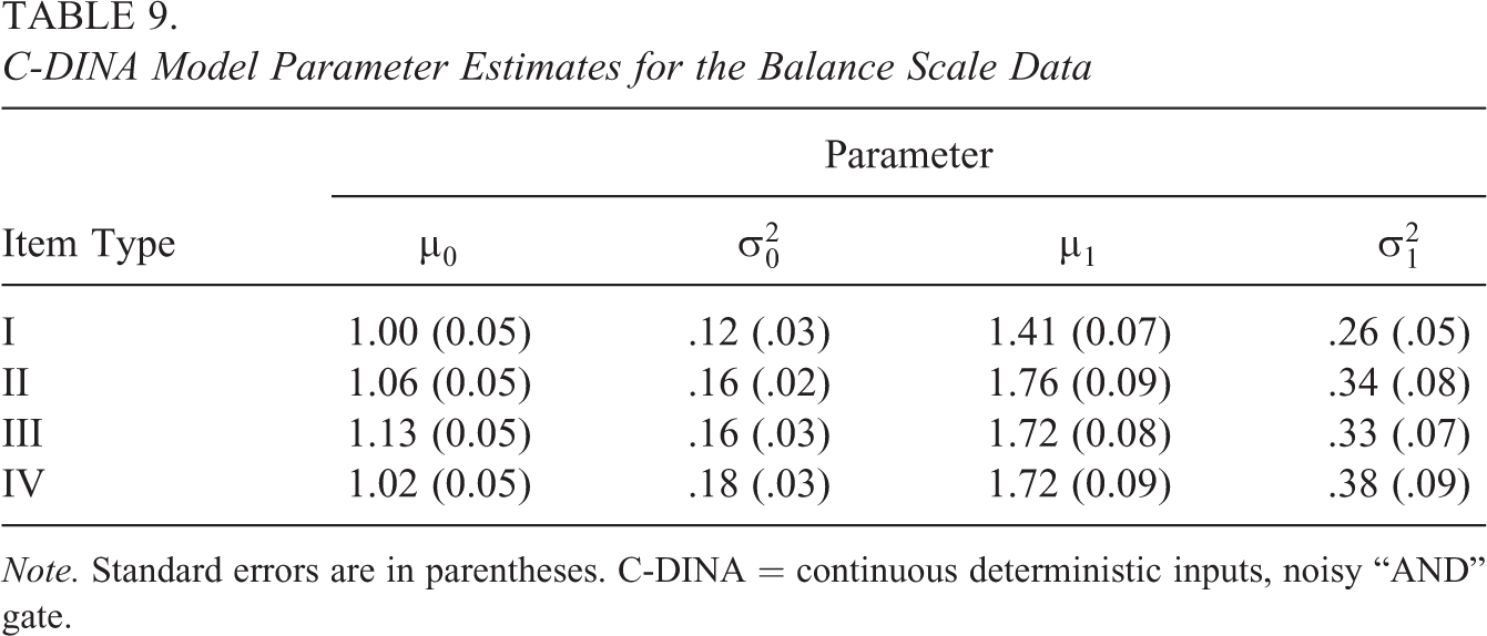
Note. Standard errors are in parentheses. C-DINA = continuous deterministic inputs, noisy “AND” gate.
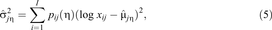
Figure 2 shows average response times by item type for each of the latent groups and classes; the plots on the left classified examinees according to their response accuracy analyzed by the DINA model, whereas the plots on the right classified examinees according to their response time analyzed by the C-DINA model. As discussed earlier, both the DINA and C-DINA models partition examinees into just two latent groups—
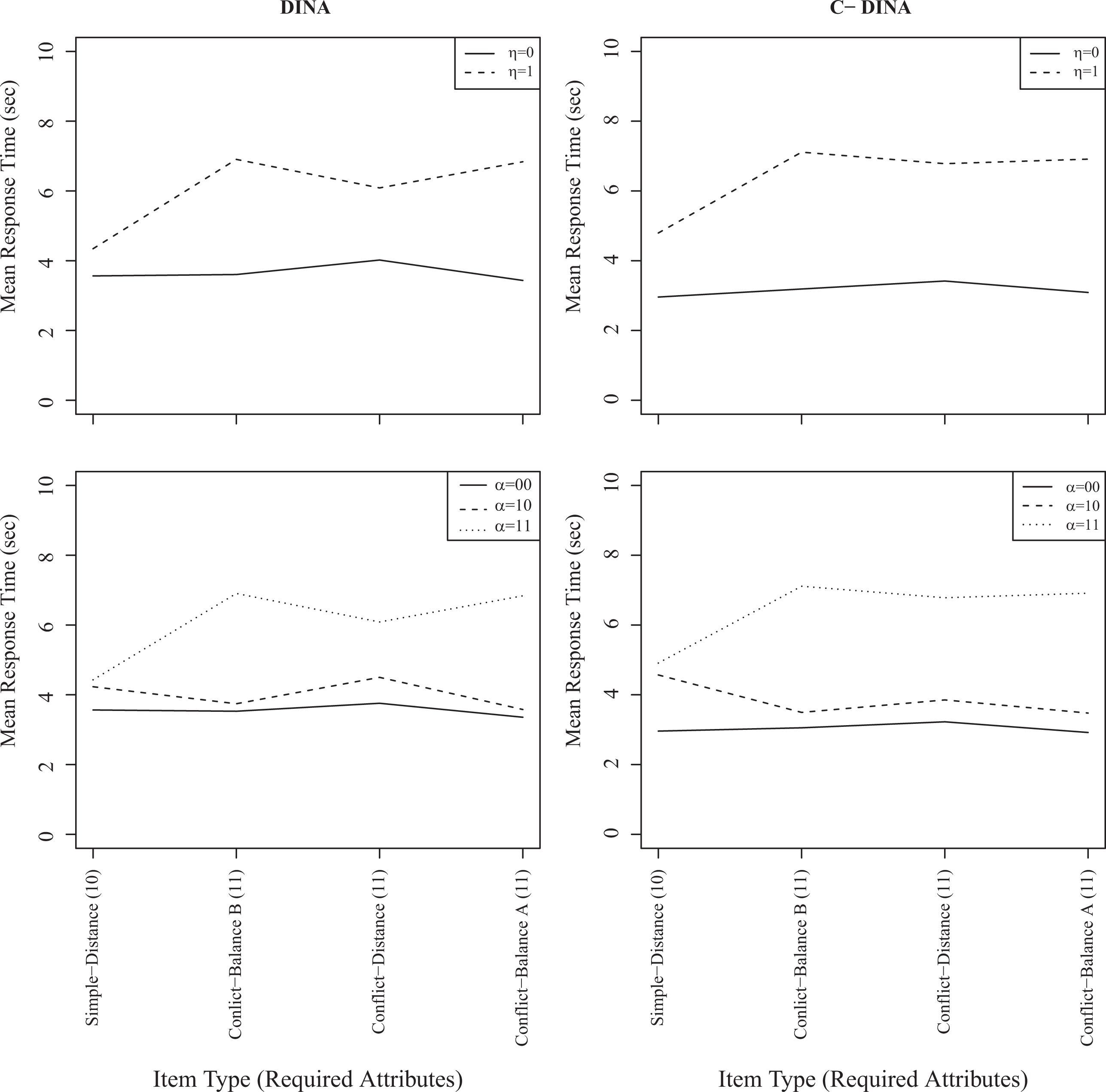
The deterministic inputs, noisy “AND” gate (DINA, left) and C-DINA (right) mean response times by latent group (upper) and class (lower).
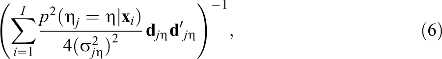
The format of Figure 3 is similar to that of Figure 2, except that it shows average response accuracy (proportion correct) rather than response time by item type for each of the latent groups and classes. Examining the top two plots, which display the proportion correct as a function of the latent groups, shows that the patterns are again quite similar, particularly for
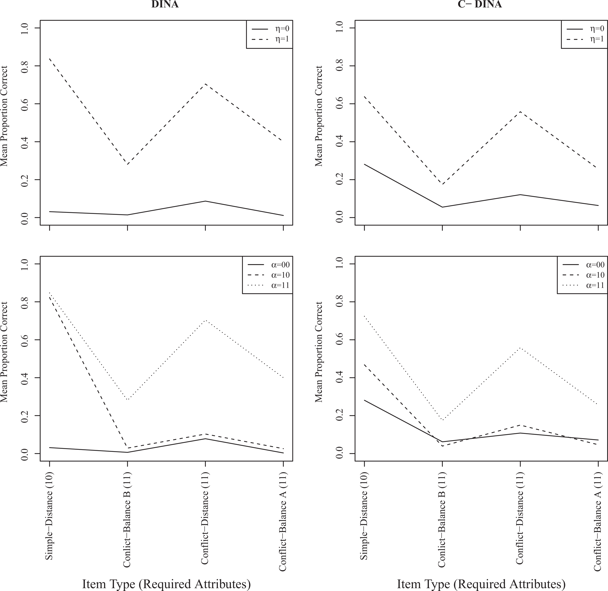
The deterministic inputs, noisy “AND” gate (DINA, left) and C-DINA (right) mean proportions correct by latent group (upper) and class (lower).
In examining the figure on the bottom left, the
Lastly, Table 10 shows the cross tabulation of the classifications for the two models. There were 92 students (63%) who had the same classifications for both models. Classifications that differed by only one attribute were observed for 37 students (25%), and the remaining 17 students (12%) had classifications that differed on both attributes. These data provide rich information into the response processes for students.
Confusion Matrix for DINA and C-DINA Classifications
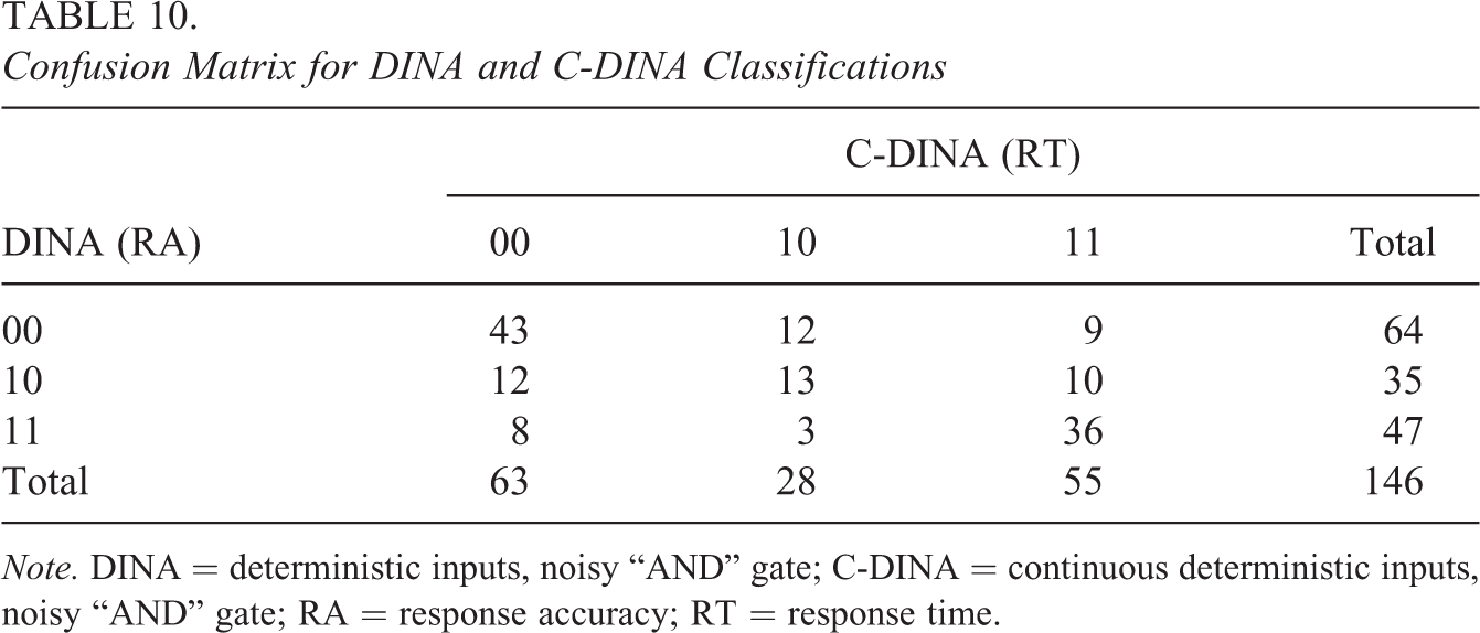
Note. DINA = deterministic inputs, noisy “AND” gate; C-DINA = continuous deterministic inputs, noisy “AND” gate; RA = response accuracy; RT = response time.
Let
6. Discussion and Conclusion
As computer-based testing becomes more prevalent, continuous response data will continue to become more readily available. This article proposed the C-DINA model, a CDM for continuous response. With the C-DINA model, latent variable modeling of continuous response data need not be based on IRT models that rely on a single continuous trait, which can only indicate a respondent’s overall standing. As an alternative, these data can be analyzed using models that can provide more specific information regarding the respondent’s standing in a multidimensional space. As with CDMs for discrete data, the C-DINA model has the potential to provide inferences that are richer and more informative and thus more useful from both theoretical and practical perspectives.
The simulation study supported the viability of the proposed model. Using the computer code based on an implementation of the EM algorithm, the study showed that reasonable estimates of the C-DINA model parameters can be obtained even with a relatively small sample size. A larger sample size is recommended if parameter estimates of greater precision are desired or if tests with less discriminating items are involved. All four parameters were affected by sample size and discrimination, whereas test length primarily affected
Applying the DINA and C-DINA models to the response times on the balance scale tasks revealed several interesting findings. By applying the expectation and variance formulas for the lognormal distribution, the estimated model parameters revealed both the mean and the variability of the response times across the different item types, allowing for inferences to be made about the characteristics of the responses of each group (i.e.,
The cross tabulation of classification showed that the classifications for the models were related, although they were not identical. This provides a basis for using one response type to augment the other, although further study is needed. It can also be used to better understand why certain groups of examinees respond in a particular way. Some groups of examinees appeared to understand certain concepts based on their response time, but failed to implement them correctly. Conversely, other students appeared to solve complex item types very quickly. These observations underscore a practical matter when applying the C-DINA model: If educators are interested in response time but response accuracy is inherently valuable, a dual analysis of the response accuracy and the response time should be performed. Such an analysis provides richer information than a single-response analysis.
The work represented in this article is an initial attempt at better understanding continuous response from a cognitive diagnosis perspective. Although it broadens our understanding of the proposed model in particular and cognitive diagnosis modeling of continuous data in general, a lot of work remains to be done in this area.
First, the current setup of the simulation study presented in this article was limited in many ways. In particular, the number of attributes, the parameters of the items for a given discrimination condition, and the Q-matrix were all fixed in this study. In future studies, they can be considered as additional factors, and their impact on item parameters estimates and attribute classification accuracy in the continuous response context should be examined. Next, the assumption of the C-DINA model used to formulate Equation 2 can be relaxed, and its formulation can be generalized in a manner analogous to the way that the DINA model was generalized by de la Torre (2011). In such a model, each item partitions examinees into
Third, additional work needs to be done in examining the fit of the C-DINA model, particularly to real data. The inferences based on this model are only valid to the extent to which it provides an adequate fit to the data. One way of examining model–data fit is to validate the Q-matrix specifications. For example, de la Torre (2008) developed an empirical Q-matrix validation method for the DINA model, and de la Torre and Chiu (2016) extended this method to the G-DINA (de la Torre, 2011) model. Similarly, Q-matrix validation methods could be developed for the standard or generalized version of the C-DINA model.
Finally, the current formulation of the C-DINA model limits its application strictly to continuous response. As alluded to earlier, the model can be extended to handle continuous and dichotomous data simultaneously. Such a model can build upon the work of van der Linden (2007), whose model from a hierarchical IRT framework can simultaneously handle both the latency and the correctness of the response.