
Abstract
Ecological momentary assessment (EMA) is a popular assessment method in psychology that aims to capture events, emotions, and cognitions in real time, usually repeatedly throughout the day. Because EMA typically involves more intensive monitoring than traditional assessment methods, missing data are commonly an issue and this missingness may bias results. EMA can involve two types of missing data: known missingness, arising from nonresponse to scheduled prompts, and hidden missingness, arising from nonreporting of focal events (e.g., an urge to smoke or a meal). Prior research on missing data in EMA has focused almost exclusively on nonresponse to scheduled prompts. In this study, we introduce a scaled inverse probability weighting approach to assess the risk of bias due to nonreporting of events due to fatigue on estimates of exposure or correlates of exposure. In our proposed approach, the inverse probability is the estimated probability of compliance with random prompts from a model that uses participant and contextual factors to predict this compliance and a fatigue factor that adjusts for attrition in event reporting over time. We demonstrate the use and utility of our bias assessment method with the Tracking and Recording Alcohol Communications Study, an EMA study of adolescent exposure to alcohol advertising.
The boom in communication technology is making mobile data collection an increasingly popular tool for behavioral scientists and transforming the way behavioral research is conducted. One sign of this transformation is the growing interest in ecological momentary assessment (EMA). EMA is a method of data collection in which study participants are asked to report information about their experience in a natural setting often several times a day over a number of days (Courvoisier, Eid, & Lischetzke, 2012; Shiffman & Stone, 1998). Researchers have used EMA to study urges to smoke, eating behavior, pain, emotions, and other behavioral processes (Shiffman et al., 2002; Steptoe & Wardle, 2011; Thomas, Doshi, Crosby, & Lowe, 2011).
Some EMA designs require participants to complete a brief survey at regularly scheduled or random prompts delivered throughout an extended monitoring period. This type of design allows researchers to obtain repeated samples of a participant’s thoughts or feelings and the context surrounding them (Shiffman, 2007; Shiffman, Stone, & Hufford, 2008). Other EMA designs link assessments to events, asking participants to initiate a survey whenever they experience a specified event (Moskowitz & Sadikaj, 2012).
In the current article, we focus on issues unique to a third, commonly used EMA design that involves both random prompts and event-driven reporting (Shiffman, 2007; Shiffman et al., 2008). The data we use come from a study of alcohol advertising in which youth were asked to report every alcohol advertisement that they encountered over a 2-week period and complete a short survey assessing their alcohol-related beliefs at the time of exposure. Participants in this study were also asked to complete similar surveys in response to random prompts throughout the 2-week study period. Alcohol-related beliefs measured at these random points serve as “no exposure controls” against which beliefs reported at moments of exposure to advertising are compared. This quasi-experimental design helps assess possible exposure-related shifts in beliefs and has the advantage of tapping these hypothesized shifts in real time and on multiple occasions. Studies that employ this type of design provide greater detail about dynamic behavioral processes than traditional methods, and provide rich opportunities for testing a wide variety of behavioral hypotheses (Shiffman, 2007).
Despite its numerous advantages, EMA requires considerable effort from participants, often over an extended period of days or weeks. Participants must carry and maintain an electronic device and interrupt their activities to log reports. Thus, use of this method is likely to result in considerable amounts of missing data. Failure to address missing data could result in biased inferences and misleading conclusions about study findings.
There is a large literature on methods for dealing with missing data. Most missing data problems begin with the classification of the missingness mechanism into one of the three types—missing completely at random, missing at random (MAR), and not MAR—following the framework of Rubin (1996). Methods of statistical analysis in the presence of each of these types of missingness have been developed for numerous study designs. However, the majority of these methods assume that the investigator knows when data are missing and that the main challenge is understanding the cause of missingness, such as would be the case if a participant skips an item on a survey, fails to show up for a scheduled interview, or fails to respond to a scheduled EMA prompt. In EMA studies that involve event-driven reporting, the occurrence of events is typically unknown to the researcher. For example, if a participant in a study of smoking urges fails to report some urges (perhaps when it is inconvenient or embarrassing to do so), the researcher has no way of knowing that these events and their accompanying surveys are missing. When occurrences of missing data are hidden from the researcher, standard approaches to handling missing data are not applicable.
Prior research on nonreporting in EMA studies has focused almost exclusively on compliance with random prompts. Across populations studied using EMA, such compliance is highly variable ranging from 50% to 90% (Shiffman, 2009). The reasons for these differences are only beginning to be elucidated. Sokolovsky, Mermelstein, and Hedeker (2014) present an ecological model for compliance to random prompts, with multiple factors to explain variation in compliance. Their model describes compliance as the outcome of fixed factors, such as a participant’s age or gender, and transitory factors, such as a participant’s mood or setting at the moment a prompt occurs. In their study of smoking behavior in high school students, Sokolovsky et al. found that several behavioral and demographic factors—for example, a history of alcohol use and male gender—were associated with the overall rate of compliance to five to seven daily random prompts during a 7-day period. Additionally, several contextual factors, such as being outside of the home, were predictive of nonresponse to individual random prompts. Another study of EMA compliance examined predictors of overall compliance (the proportion of all assessments that were completed) and prompt-level compliance among university students participating in an EMA study of mood (Courvoisier et al., 2012). This study found evidence of a “fatigue effect” (i.e., a drop-off in compliance as the study progressed) but no differences in compliance based on participant characteristics.
This prior work has helped to identify potential factors that could influence response to prompted assessments for certain participant populations under intensive monitoring. Much less is understood about the nonreporting of events that are not scheduled. In this article, we describe a method to correct for nonreporting suggested by nonuniform temporal patterns in event reports such as would arise from reporting fatigue. The main purpose of this method is to assess the risk of potential bias due to reporting fatigue.
The Tracking and Recording Alcohol Communications (TRAC) Study
The TRAC study used an EMA design to investigate momentary shifts in youths’ alcohol-related attitudes and cognitions that may occur in response to real-world exposures to alcohol advertisements at the time of exposure, and to link any such shifts to changes in drinking behavior over time. TRAC was a 2-year longitudinal study that enrolled over 600 middle school students from two large school districts in Southern California. At baseline and 8, 16, and 24 months after baseline, students completed a paper survey that asked about demographics, social context (e.g., parental and peer influences), and drinking behavior. Each paper assessment was followed by a 2-week period of event sampling during which students were asked to report, via handheld electronic devices, any alcohol advertising that they observed. The present study focuses on the baseline EMA data collection that occurred from September 2013 to June 2014.
Two types of survey were programmed on the handheld devices: random prompt surveys and exposure-related “event” surveys. Both types of survey assessed participants’ alcohol-related beliefs. Event surveys additionally collected information about the advertisements seen by participants. Random prompts occurred 3 times per day—once each in the morning, afternoon, and evening, outside of school hours—and were signaled by an electronic alert.
At the start of the study, participants underwent a 1-day training session on the operation of the handheld devices (five different models of Android-based phones). As part of the training, participants were instructed to keep their device turned on at all times, charge the device at night while they slept, initiate data entry each time they encountered an alcohol advertisement, and respond to random prompts when issued by the device.
All participants earned US$60 for completing the baseline questionnaire, attending training, and carrying the device for 14 days. Participants who responded to 76% to 84% of the random prompts received an additional $25; participants who responded to ≥85% of the random prompts received an additional $60.
Observed and Hidden Nonreporting
For scheduled EMA surveys, nonreporting is known exactly: Study participants either respond to the scheduled survey when prompted or they do not. Figure 1a depicts the response rate to random prompts for the baseline wave of data collection for the TRAC study. This figure shows that the overall response rate of 66% (two of the three scheduled surveys per day) was approximately constant throughout the 14-day data collection period.
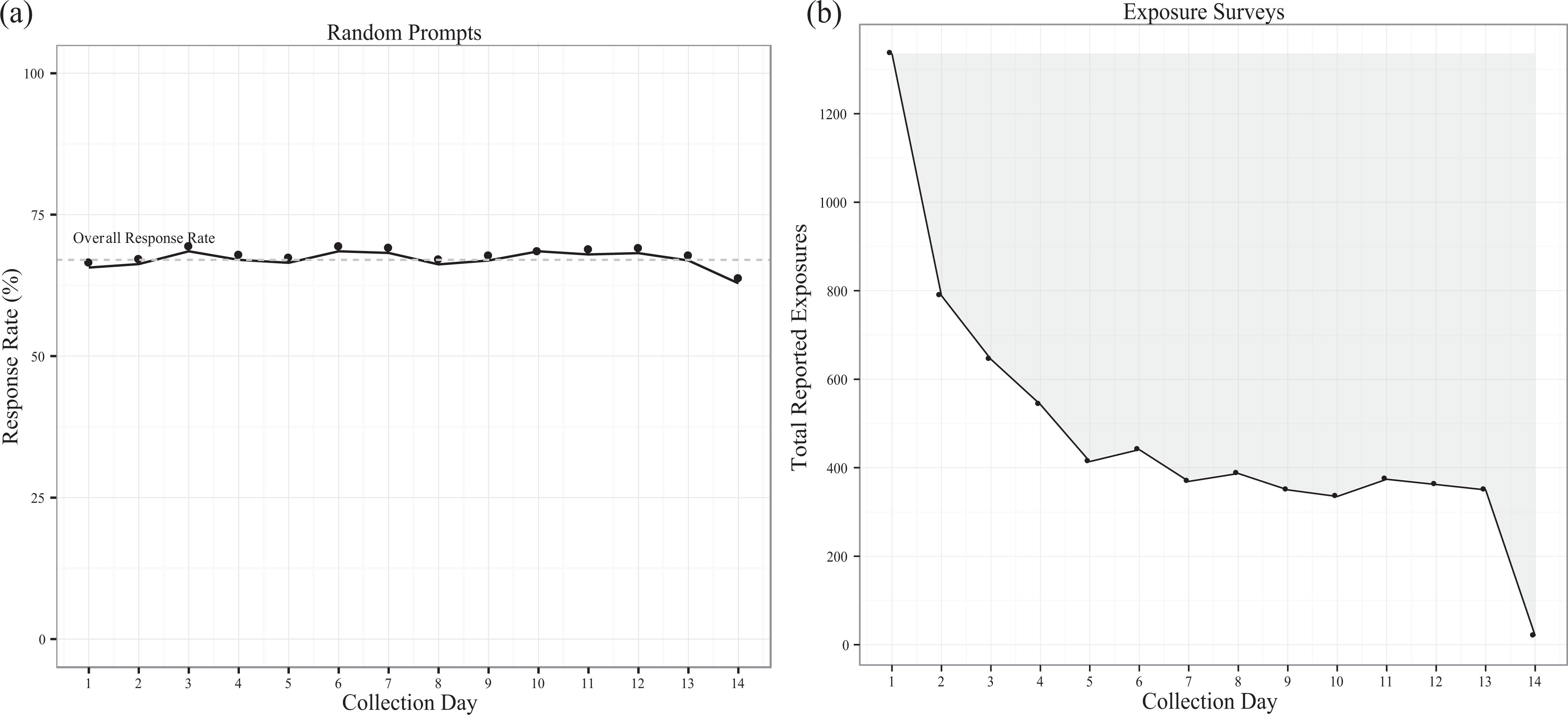
(a) Compliance with random prompts by day from start of data collection. (b) Total exposures by day from start of data collection. The shaded region denotes suspected nonreporting of exposures.
Evaluating nonreporting of events (exposure to advertisements) is more challenging. Because the occurrence of these events is not known, we cannot identify when event-triggered reports are missing. However, we believe information can be gained by identifying variables that are related to event reporting. The primary example of such a variable, and the one that will be the main focus of this article, is the day of data collection (1–14). TRAC participants were recruited throughout the week. Thus, the day of the week (Monday–Sunday) on which each participant began reporting exposures to alcohol advertisements was random. This feature of the design was integral to the study, since television watching and alcohol advertising on television vary by day of the week. Because the day of the week that participants began is random and variable, we should expect to observe a similar number of exposures to alcohol advertisements being reported on each day (1–14) of data collection. However, a plot of total reported exposures by data collection day shows a sharp drop in the number of alcohol advertisements reported with each passing day in the first 7 days of monitoring, followed by a steadier but lower total during the second 7 days (see Figure 1b).
The pattern of reported exposures to alcohol advertisements and responses to random prompts suggests several things about nonreporting of events in the TRAC study. First, there is evidence of a fatigue effect, that is, students reported advertisements more often earlier versus later in the data collection period. Second, there is no evidence of fatigue in response to the random prompts, suggesting that responsiveness to random prompts and reporting of exposures involve different processes. Below, we present a conceptual model that can account for this.
Conceptual Model of Nonreporting in EMA
Our conceptual model of nonreporting in EMA is based in part on the social–cognitive framework proposed by Sokolovsky and colleagues (2014). According to this model, the decision to complete an assessment is influenced by participant characteristics, the demands associated with reporting, and contextual effects (see Figure 2). The inclusion of participant characteristics in the model allows for the possibility that certain types of individuals might be more likely to comply with an EMA protocol than others, for example, participants who are more conscientious in general might be more likely to complete assessments than participants who are less conscientious in general. Reporting demands refer to the behaviors or requirements of reporting such as length of the survey instrument. Contextual effects are features of the situation in which reportable events occur that may influence the reporting of that event. Time of day and the presence of other individuals are some examples of such factors.
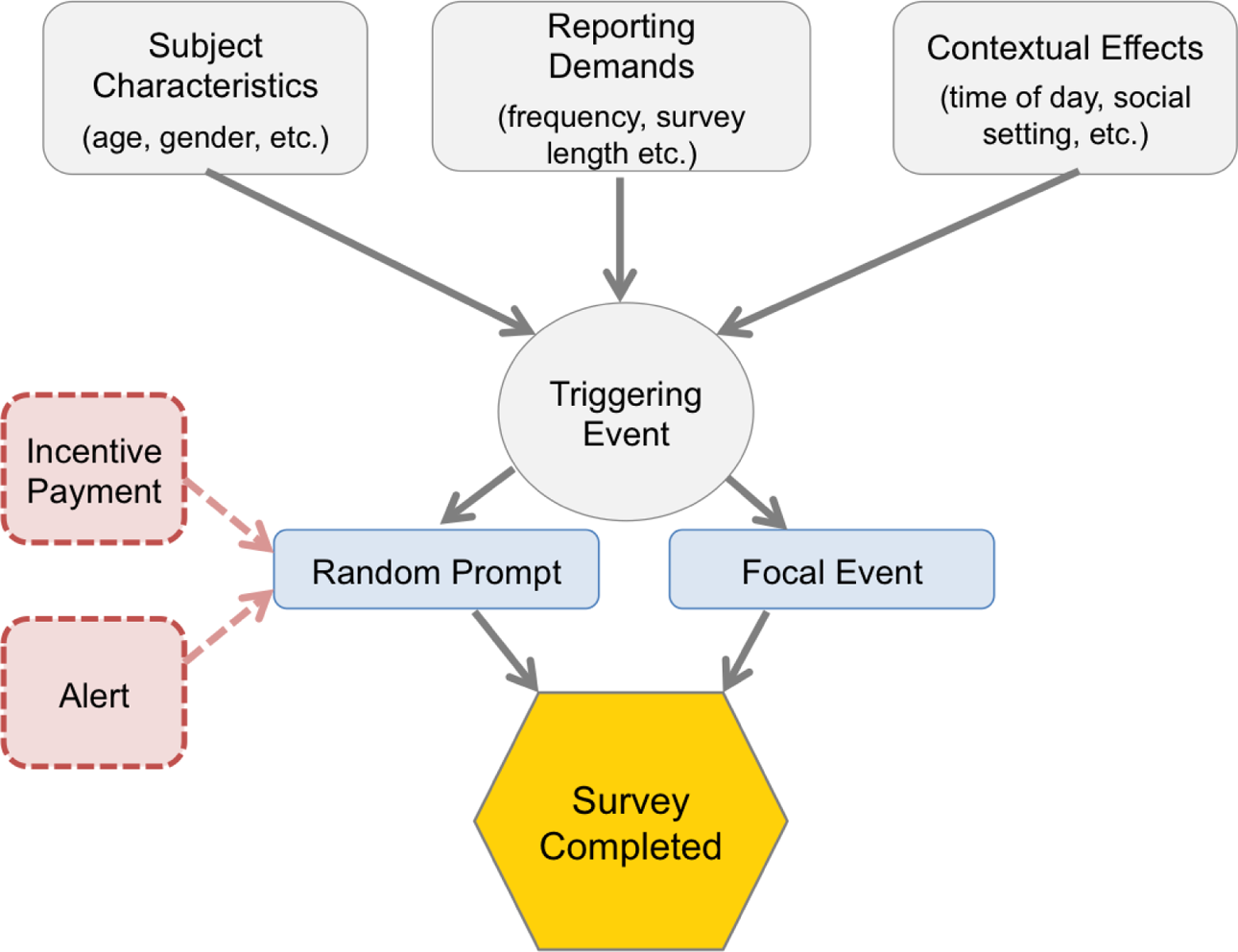
Conceptual model of reporting in an ecological momentary assessment study.
Based on the observed differences in response to scheduled prompts and event-triggered reports in TRAC, we expand this conceptual framework to include scheduled assessments (random prompts) and reportable events as distinct triggering events. Responses to both events are assumed to be under the influence of the same participant, reporting, and contextual effects; however, by separating the triggering events into random prompts and focal events, each event can have additional, unique influential factors. For example, random prompts, unlike reportable events, frequently are accompanied by alerts and provide the basis for incentive payments.
Not included in the conceptual model are response effects related to the characteristics of the reportable event itself. Such effects are distinct from the context in which the event occurs but relate specifically to characteristics of the event itself. For example, in the case of alcohol advertisements, commercials for alcoholic beverages that are made to appear like energy drinks might be less recognizable as alcohol advertisements than commercials for other beverages. We do not include characteristics of the event itself in our conceptual model because we assume that after accounting for participant, reporting, and contextual effects, the properties of events and the reporting of those events are conditionally independent.
In the following section, we develop a statistical model that builds on our conceptual framework of reporting in EMA. This model will be used to evaluate evidence of event nonreporting and the risk of bias in estimates of exposure and correlates of exposure.
Statistical Model
Notation and Terminology
To represent the TRAC EMA data, we will use
Model
We consider the problem of estimating the number of events experienced by participants in an EMA study when it is suspected that some experienced events have not been reported by study participants (i.e., there is nonreporting). To formalize the problem, we suppose that each experienced event has a probability of being reported,
The use of weights to “weigh back” to the source population (in the present case, the population of ad exposures) is directly related to design-based methods in survey research in which sampling weights that represent the inverse probability of inclusion in the sample (with possible correction for nonreporting) are used to estimate population parameters (Groves, 2002; Korn & Graubard, 1995). Whereas weights in the survey setting are typically known and determined by the survey design, reporting weights for EMA must be estimated. The key challenge in estimating response weights with event-based EMA is the unknown incidence of targeted events. EMA researchers have information about the events subjects choose to report, but (typically) no information about the events subjects do not report. Consequently, traditional missing data problems using imputation are not applicable.
In our proposed model, the likelihood of reporting an experienced event is a function of the tendency to comply with study instructions and reporting fatigue, which can be measured from information about subjects’ compliance to scheduled assessments and temporal trends in the reporting of exposure events. In conceptual terms, the model for the reporting weight—the inverse of the probability of reporting an experienced eligible event—can be described as follows: reporting weight = compliance weight × fatigue effect
The reporting weight is composed of two components: a compliance weight, which is equal to the inverse of the probability of completing a scheduled (random prompt) assessment, and a fatigue effect, which describes the decreased likelihood of reporting experienced events over time. Because the fatigue effect can be regarded as a scaling factor applied to the inverse probability of compliance, we refer to the reporting weight as a scaled inverse probability weight (SIPW).
The mathematical representation of the SIPW model uses wi
(t) to represent the reporting weight for the reported exposure at time t for the ith subject. The compliance weight for the ith subject at time t is denoted

Here, the fatigue effect is described more fully by
The compliance component of the model,

Equation 2 shows that the estimated compliance weight is the inverse of the expected compliance probability given subject and contextual factors
Unlike compliance, fatigue patterns cannot be observed at the subject level. This is because the events that are the focus of EMA studies are not under the control of the researcher, and the actual incidence of these events is unknown. Instead, the pattern of event reports for any one subject is dictated by the level of actual exposure and the subject’s willingness to report over time, and it is not possible for the researcher to disentangle these two factors influencing reporting at the subject level. Instead, under assumptions detailed in the next section, the fatigue effect can be estimated from the aggregate reporting patterns for a group of subjects.
Assumptions
There are two main assumptions underlying the validity of the response model in Equation 1. The first assumption is that exposure reports are MAR, which means that the mechanism behind missed reports can be explained by observed subject and contextual factors,
Estimation
We propose a two-stage procedure for estimating the parameters of the SIPW model. The first stage involves the selection and fitting of the model of compliance with random prompts. In the second stage, we specify the group-level model for the fatigue effects, α.
To estimate the expected probability of compliance, we fit the following hierarchical linear regression model:

The fixed effects of time-varying and time-fixed effects are represented by the parameters γ, while
The second stage of modeling is the specification of the fatigue model. Given the pattern observed in TRAC (Figure 1b), we propose a stratified model for the fatigue factor that varies with the day of study collection, d, and a set of K subject strata,

In Equation 4,
A nonparametric estimate for the α parameters of Equation 4 can be obtained by simply inserting the strata-specific exposure counts for

where
When multiple models for the fatigue effects are considered, we use a goodness-of-fit criterion to identify the best-performing model. In this article, we use Pearson’s χ2 goodness-of-fit measure and its associated χ2 test. The form of the statistic is
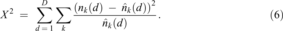
Smaller values of
Reducing Bias Due to Reporting Fatigue
Once the compliance and fatigue model parameters have been estimated, their values are substituted into Equation 1 to estimate the final response weights. These weights can be incorporated into estimates of exposure levels or correlates of exposure. As a simple illustration of the construction of the weights, we use a hypothetical example of reporting fatigue in Table 1, where exposure reporting decreases at a constant rate of 10% per day. The response weights are derived from the pattern observed in total reported exposures per day. The weights are applied to estimate the proportion of exposures per day and total exposures. Large differences in the unweighted and weighted estimates would suggest evidence of reporting fatigue and a high risk of bias. In this example, there is a 30% difference in the unweighted and weighted estimates of total exposure, suggesting the presence of nonnegligible nonreporting.
Illustration of Response Weight Correction With Hypothetical 10% Cumulative Reporting Fatigue per Day
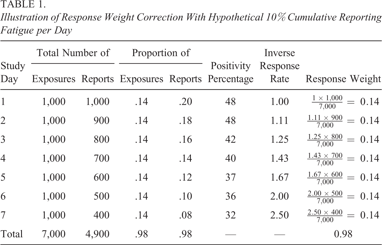
Weighting for nonreporting is important not only for assessing potential bias in estimates of amount of exposure but also for estimating correlates of exposure. For example, suppose that the outcome of interest is a positive impression of an alcohol advertisement and that the true probability of a positive impression is 40%. If the percentage of positive impressions of observed reports is as shown in Table 1, the unweighted estimate of positivity across the 7 days would be 42%. The weighted estimate (Horvitz & Thompson, 1952) of positivity using the correction for possible reporting fatigue would be 40%.
Inference
The main goals of this article’s motivating EMA study are to describe characteristics of exposure to alcohol advertisements and the effects of those exposures on beliefs. We suppose that the parameter of interest can be expressed as the solution to the minimization problem:
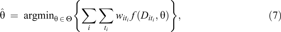
where

A simple extension of this regression model would provide an estimate of the unadjusted effect of exposure on the outcome of interest,
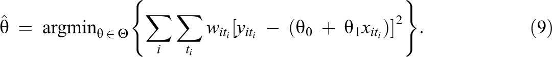
In place of the unknown response weights,
Resampling CI
Calculation of the CI for Let D represent the complete data and set Obtain estimated weights based on the observations from the resample, Obtain the estimated Repeat Steps 1–3 for To construct the
A similar approach can be used to obtain other quantities of the sampling distribution of
Reporting
An assessment for event nonreporting should be a routine part of sensitivity analyses performed with EMA studies. Reporting practice should follow published guidelines for sensitivity analyses (Thabane et al., 2013). The assessment should include a description of the analytic approach for evaluating nonreporting in the Methods section of the report, including details of the compliance and fatigue models, predictors included, and measures of model fit used. The Results section should include a summary of the evidence of nonreporting and its possible impact on the study findings. Where small differences are found, this could be a brief statement in the text. For larger differences, we recommend that both the observed and fatigue-corrected estimates be displayed and described and that a discussion of the limitations and implications suggested by these differences be included in the Discussion section of the report.
Application
Participants
The TRAC sample consists of six hundred six 11- to 15-year-olds from the Los Angeles area. The sample is racially and ethnically diverse: 26% identified as Hispanic and 29% as Black (Table 2). The majority of students (62%) stated that they lived with both their mother and their father. Less than a quarter of participants said that they had tried alcohol (even a few sips).
Baseline Characteristics of Sample
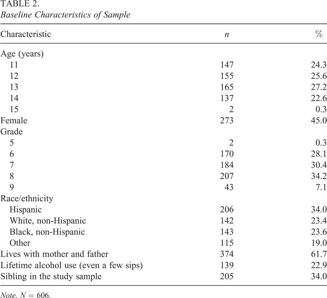
Note. N = 606.
Predictors of Compliance
We define compliance as the completion of a scheduled (random prompt) survey. As shown in Figure 1a, the average compliance rate was 67%, and there was no significant variation in compliance over the 2-week period of data collection. We used a hierarchical generalized linear regression model to determine whether compliance was associated with key baseline characteristics. The hierarchical model allowed us to account for clustering of siblings within families (n = 205) and assessments within individuals using nested random effects. The outcome of the regression model was an indicator for whether a scheduled random prompt was completed (completed = 1 and not completed = 0). There was a total of 42 scheduled random prompts per subject (3 planned prompts per day for 14 days), and the model’s error distribution was binomial with a logistic link function. In keeping with our conceptual model, we considered participant characteristics that focused on factors related to conscientiousness—history of drinking, grades in school, value on academic achievement, religiosity, and rebelliousness—along with several student demographics: age, gender, race/ethnicity, and household composition. We also considered mental health, as we suspected it might be related to reporting fatigue. Because grade in school and age are highly correlated, only age was considered.
All items were based on student self-report. Grades in school were assessed with a single item with four response options (1 = below average to 4 = excellent). Value on academic achievement was the mean of 2 items (α = .66) adapted from Donovan and Molina (2011): “How important is it to you to get good grades at school?” and “How important is it to you to get high scores on your tests at school (1 = not too important to 3 = very important)?” Religiosity was assessed with a single categorical item: “Religion is very important in my life (1 = strongly disagree to 5 = strongly agree).” Poor mental health was the mean of responses to 5 scaled items from the 36-item Short Form Health Survey (SF-36) (Ware, Kosinski, & Dewey, 2003). Specifically, participants were asked, “In the past month, how much of the time have you been a nervous person,” “felt calm and peaceful,” “felt downhearted and blue,” “been a happy person,” and “felt so down that nothing could cheer you up (1 = none of the time to 6 = all of the time)?” Responses to these items were coded so that higher values indicate worse mental health and averaged to create a measure of poor mental health (α = .62). Finally, rebelliousness was the log transformation of the number of endorsed items of 6 items: “I get in trouble at school,” “I argue a lot with other kids,” “I do things my parents wouldn’t want me to do,” “I sometimes take things that don’t belong to me,” “I argue with my teachers,” and “I like to break the rules” (Sargent et al., 2004).
Modeling compliance at the level of the scheduled assessments allowed us to incorporate time-varying factors as well as time-fixed factors. We anticipated that willingness to comply could vary with the time of day, day of week, and period of data collection. To examine the influence of each of the factors, we included the period of day of each scheduled assessment using a three-group categorical variable with categories for “morning,” “afternoon,” and “evening.” A categorical indicator for weekends (Friday–Sunday) was also included, as was an indicator for the second week of data collection.
Several exclusions were made prior to analysis. We omitted the data from 18 students who had had a defective device (n = 5), withdrew from the study (n = 1), or failed to complete a scheduled assessment (n = 12). Also, the large drop in exposures reported on the 14th day of data collection (Figure 1b) suggests that students thought the collection period had ended by the 13th day. We therefore only examine reporting on the first 13 days of collection, which included a total of 39 scheduled (prompted) assessments.
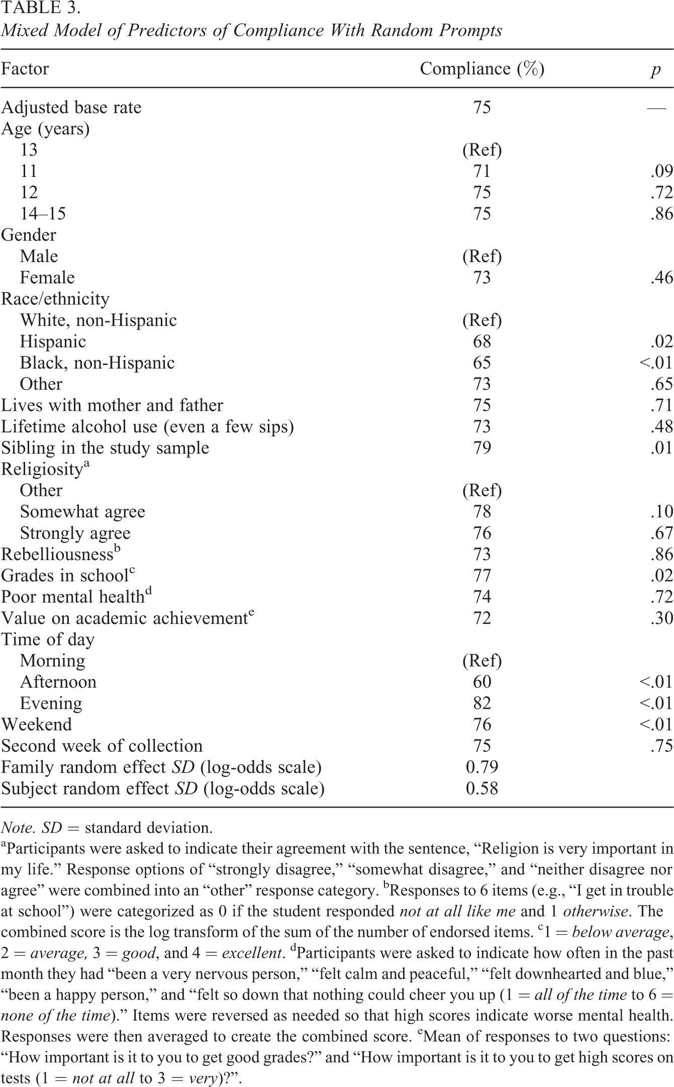
Table 3 shows that race and ethnicity were strongly associated with compliance, with both Hispanic and non-Hispanic Black students exhibiting lower observed rates of compliance than Whites (−5.8% and −8.1%, respectively). Getting good grades in school was associated with a 3.3 percentage point increase in compliance rate. Clustering among siblings accounted for 39% of variation in compliance and had a nonsignificant positive marginal effect of 4.4%.
Mixed Model of Predictors of Compliance With Random Prompts
Note. SD = standard deviation.
aParticipants were asked to indicate their agreement with the sentence, “Religion is very important in my life.” Response options of “strongly disagree,” “somewhat disagree,” and “neither disagree nor agree” were combined into an “other” response category. bResponses to 6 items (e.g., “I get in trouble at school”) were categorized as 0 if the student responded not at all like me and 1 otherwise. The combined score is the log transform of the sum of the number of endorsed items. c1 = below average, 2 = average, 3 = good, and 4 = excellent. dParticipants were asked to indicate how often in the past month they had “been a very nervous person,” “felt calm and peaceful,” “felt downhearted and blue,” “been a happy person,” and “felt so down that nothing could cheer you up (1 = all of the time to 6 = none of the time).” Items were reversed as needed so that high scores indicate worse mental health. Responses were then averaged to create the combined score. eMean of responses to two questions: “How important is it to you to get good grades?” and “How important is it to you to get high scores on tests (1 = not at all to 3 = very)?”.
We applied a stepwise backward regression approach with a 25% significance criterion to select factors to include in the compliance model (Equation 3) for the TRAC study. A more lenient significance criterion than the standard 5% level was used to avoid risk of bias due to omitting predictors of compliance (Collins, Schafer, & Kam, 2001). This resulted in a mixed logistic probability model with nested random effects for family and subject; fixed subject effects for race, academic achievement, having a sibling in the sample, religiosity; and fixed time effects for the time of day and time of week (weekday or weekend) of the scheduled assessments.
Scaling for Fatigue
We considered a number of parametric models to obtain estimates for the fatigue factor,
To allow for possible overreporting on the first day, we evaluated the fit of the parametric models excluding the first day of collection and chose the model with the best fit to the observed total exposures for these days. This allowed us to see whether the evidence from the remaining days is inconsistent with the first day under a specific model. A higher than expected count on the first day would be suggestive of overreporting, though not conclusive as it is only assumed that the model fit to the remaining days is correct.
The models included a linear model with log-transformed counts and days (log-log linear), the same model with an additional quadratic term for log-days (log-log quadratic), a loess, and a model of days on the inverse count (which was the optimal Box–Cox transformation for the data). Several stratified models were also considered, each using the log-log linear model. The stratification variables included weekend (vs. weekday), time of day, and week of monitoring (first or second). In addition to fitting the models to the full data, we removed the data point for the first day, denoting these models with −1. We note that the loess model could not be considered in this case, as extrapolation from the curve would not be possible.
Table 4 summarizes the goodness of fit of a subset of the fatigue models that we considered. We also considered models that allowed for variation in fatigue by student rebelliousness, academic achievement, and mental health. Because the performance of these more fully adjusted models was consistently poorer than the model that only considered period effects, we present them in the Online Supplementary Material (Online Supplementary Table S1).
Goodness of Fit of Evaluated Fatigue Models
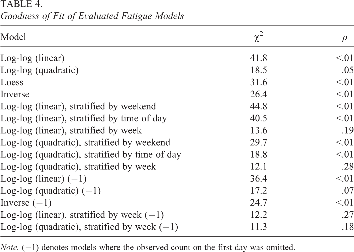
Note. (−1) denotes models where the observed count on the first day was omitted.
Among the unstratified models, the log-log quadratic showed the best overall fit. When we stratified this model by week, allowing a separate polynomial for the first and second week, it greatly improved the fit of the model. Omitting the first day from the data set further improved the fit of the polynomial model, an inconsistency under that model that suggested the presence of overreporting on the first day.
The components used to construct the final weights are described in Table 5. To allow for overreporting on the first day of collection, the scaling factor for the first day is set equal to
Summary of SIPWs for Compliance by Study Collection Day
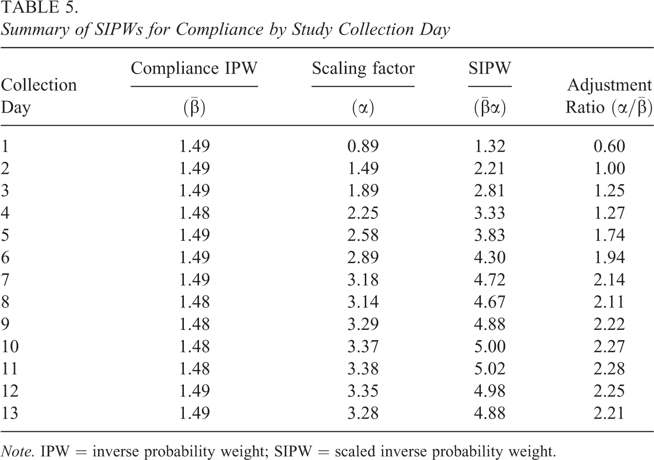
Note. IPW = inverse probability weight; SIPW = scaled inverse probability weight.
Estimated Positivity Toward Ads
Using the selection weights derived above, we conducted a bias assessment for event nonreporting with estimates of positivity toward advertisements. With each reported exposure, participants were asked whether they “liked the advertisement.” We defined a positive response as either “somewhat agree” or “strongly agree.” Table 6 shows that the observed positivity toward ads was 14.5% (95% CI [12.4, 16.8]) overall. The most positive responses were to radio advertisements and branded specialty items (e.g., hats), with each having a mean percentage of positive responses greater than 20%; the lowest percentage of positive responses was found for product placements, which garnered no positive responses.
Risk of Bias in Frequency of Positive Response to Advertising
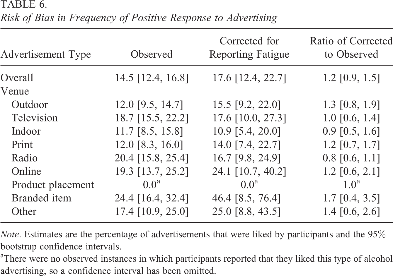
Note. Estimates are the percentage of advertisements that were liked by participants and the 95% bootstrap confidence intervals.
aThere were no observed instances in which participants reported that they liked this type of alcohol advertising, so a confidence interval has been omitted.
The risk of bias assessment suggested that the fatigue-corrected estimates tended to suggest greater positivity toward ads, with a 20% higher positivity estimate overall (95% CI [−10%, +60%]). The magnitude of the difference between the observed and fatigue-corrected estimates suggests that estimates of positivity were sensitive to assumptions about reporting fatigue and would generally underestimate positivity if ignored. Several advertisement types showed more than a 20% change in the mean estimates of positive response with correction for reporting fatigue, including outdoor advertisements, branded specialty items, and “other” advertisement types (Table 6). Positive impressions of television advertisements and product placements showed the lowest risk of bias due to reporting fatigue overall.
Simulation
To evaluate the broader applicability of our method, we conducted a small simulation study. In this study, reporting fatigue followed a power law relationship over a range of baseline levels. The power law mimicked the fatigue effect that would be expected at the group level, that is, a gradual decline by which the most reporting occurs in the earliest days of the study and the least in the finals days of collection. A fixed compliance of 67% was assumed throughout. Applying a logistic model for compliance and the log-log quadratic model used in the above application, we found that the adjustment method accurately recovered the true level of exposure for all conditions considered (Online Supplementary Table S2). While the observed exposure level ranged from 34% to just 24% of the true level of exposure, the corrected exposure levels had an accuracy of 99% on average with an error no more than 5% for any condition considered.
Discussion
Nonreporting of events in EMA studies could threaten the validity of estimates of event frequencies and effects; yet methods to address the fundamental problem of event-based nonreporting in EMA designs have not been developed. This article seeks to address this gap by presenting a methodology to evaluate the presence and possible impact of fatigue with regard to the reporting of events in EMA studies. The method uses a scaled inverse probability weighting approach to account for the separate contributions of compliance and event nonreporting, accommodating subject, and contextual predictors for both nonresponse mechanisms. We show that adjustment for nonreporting can be a useful tool for assessing the risk of bias for estimates of frequency of exposure and correlates of exposure in the presence of reporting fatigue.
The primary objective of the method presented in this article is to correct for fatigue effects in the reporting of events in EMA studies. Our method can also help to identify and adjust for more general temporal patterns in event reporting such as potential overreporting. We found that the count on the first day of data collection was inconsistent with the model of best fit for the remaining days. One possible explanation for this inconsistency is overreporting as high as 11% on the first day of data collection. Such overreporting could be attributed to reactivity—behavioral changes in participants owing to EMA participation (Kazdin, 1974). While reactivity has generally been regarded as a fixed phenomenon (Rowan et al., 2007), the evidence from TRAC suggests that reactivity may be more temporally dependent and of greatest concern at times that are most proximal to training and/or interactions with the research staff. An additional benefit of the method in this article is that it can help to identify evidence of time-dependent reactivity, a phenomenon that has not received much empirical attention to date.
Quantifying event nonreporting is challenging because missing reports of events are usually hidden from the investigators. In this article, we demonstrate that patterns in aggregated summaries of reported events can provide useful information about temporal drop-offs in reporting, given that the day of collection in EMA is typically independent of the exposure mechanism. In the TRAC study, plots of total exposure by day revealed evidence of fatigue in exposure reporting: Total reports of advertisements were more numerous in the earlier days of data collection than in the later days. We found no such pattern in rates of compliance with random prompts. This observation suggests that the mechanisms underlying compliance to scheduled and unscheduled reporting are not identical.
Although the prevalence of reporting fatigue in EMA is not well understood, our observations in the TRAC study suggest that event nonreporting is likely to be common and, without adjustment, can lead to a misrepresentation of the behavioral process of interest and its possible effects. The extent of bias for any given application will depend on the strength of the correlation between the estimate of interest and the fatigue mechanism (Korn & Graubard, 1995). Because a researcher will not know the extent of this bias during study planning, we recommend that a post hoc assessment be routinely performed as in our application study.
Ignoring nonreporting makes the strong assumption that event reports are either not missing, in the case of estimating levels of exposure, or missing completely at random, in the case of estimating correlates of exposure. The model proposed in this study is a significant improvement in usual practice because it recognizes nonreporting of events and allows for the possibility that participant and other factors affect this nonreporting. Although the assumptions underlying our method are certainly more reasonable than assuming the absence of missing event reports, they might not be reasonable for some study designs. Thus, it is important to understand the limitations that each of our assumptions presents.
The ability to estimate the compliance and fatigue effects of the SIPW model rely on two main assumptions: that missing reports are MAR and that the level of the event of interest in the population is stable during the data collection period. The MAR assumption is common among modern approaches to missing data problems. MAR is most plausible when a large number of potential determinants of missingness can be included in the model of the missing data mechanism in a flexible way (Rubin, 1976). Our approach can accommodate a rich set of explanatory factors in both the compliance and fatigue components. Further, there are no restrictions on the form of the model for compliance. Researchers can choose from any available approach for modeling binary data.
Options for modeling fatigue in reporting are more limited because modeling has to be done on aggregate event reports, where independence between the timing of collection and the exposure mechanism holds. At the person level, the number of reported exposures could reasonably change over time, even in the absence of fatigue, due to natural patterns in a person’s interactions with their environment. This prevents the isolation of fatigue effects without more information about an individual’s actual event patterns. However, when we aggregate events across individuals, we would expect the total level of events to be stable for the group if their behaviors are independent of each other and the environmental process under study is not changing over time, conditions we define as ecological stability. The ecological stability assumption implies that the order of data collection (and any other aspect of the study design) is uncorrelated with the incidence of events. This would be expected if the time of enrollment is randomly determined, and the occurrence of the event is not directly influenced by the study.
One potential threat to ecological stability is pervasive reactivity in the form of hypervigilance toward advertisements. Data from TRAC revealed that a modest level of reactivity (in the form of overreporting) occurred on the first day of collection but not on subsequent days. For other studies, it is possible that reactivity could be more pervasive and threaten the study findings. Intervention studies that target the behavior of interest would be another example where the assumption of ecological stability might not be applicable to all treatment arms. In either of these cases, the SIPW method could be extended to include a reactivity correction, which could be estimate, for example, through the incorporation of a low-frequency monitoring group to the study design.
To allow flexibility in the fatigue model, we proposed a stratification approach and provide a goodness-of-fit measure to assist researchers in identifying explanatory factors for fatigue and selecting a final model. When there is substantial variation in the rate of fatigue within the study’s sample, a large number of strata might be considered. Guidance is available for determining the minimum sample size for stable estimation of regression models of fatigue within stratum (Harrell, 2001). A general rule of thumb is a minimum of 10p subjects per stratum for a fatigue model with p parameters; when the number of potential explanatory factors for fatigue is very large, dimension reduction methods can be employed. In addition to sample size considerations, strata should not be correlated with the day or time of enrollment, as this could introduce period effects that may violate the assumption of independence between the incidence of events and study day.
Alternative modeling approaches for the compliance and fatigue models could be considered. Handling the multilevel structure with scheduled assessments is the most challenging aspect of the compliance model. We have used a mixed effects model, which is one strategy to reduce bias in weights with clustered data. Two-stage methods and doubly robust methods could also be considered (Hong, 2010; Li, Zaslavsky, & Landrum, 2013). Whether any of these approaches is superior in the EMA context remains an open question. Overfitting is another concern for the performance of both models. Although of greatest concern for models applied to the outcome, researchers can also protect against overfitting in estimated weights using a method such as cross-validation or, more formally, with a method that directly penalizes larger models. Although models for missing data encourage the use of all available covariates to better satisfy the MAR conditions, care is needed with covariate selection when using scaled items from questionnaires that may have low reliability and/or measurement error (Lockwood & McCaffrey, 2014). Finally, we have used a two-stage procedure with empirical weights treated as known weights, which could underestimate the variability of the weighted estimates. Further development of the method could address this by incorporating the weight derivation in the resampling procedure or by estimating the weights and effects of interest in a joint model.
Because modeling to correct for reporting fatigue relies on assumptions that cannot be verified using standard data collected via EMA, we recommend that it be used as a tool for assessing risk of bias rather than as an adjustment method. If the risk of bias is not small, researchers may want to consider a confirmatory study. This could take the form of a comparison against estimates collected with an alternative method with lower risk of reporting fatigue. If such data are not available, the researcher has several options. First, a two-stage sampling could be performed in which a subsample of “nonreporters” is followed up with more intensive questioning about missing event reports. Such sampling methods are well established as a means for handling missing data (Baker, Wax, & Patterson, 1993; Frangakis & Rubin, 2001). Second, a subsample of participants could be randomly assigned to more intensive monitoring to investigate the effects of monitoring burden on reporting. Both approaches would provide a way to confirm reporting fatigue and identify other potential causes of nonreporting.
As awareness and study of EMA nonreporting grows, researchers will need new methods for preventing or reducing causes of nonreporting during data collection. The present article is a step toward more robust EMA designs in that it provides a method to evaluate the extent of nonreporting due to fatigue with standard EMA methods.
Conclusion
One of the goals of EMA is to reduce bias by reducing reliance on recall. Yet when nonreporting of events is common, missingness can undermine the conceptual strengths of the EMA methodology. It is important that EMA researchers routinely assess the presence and possible impact of noncompliance and suspected event nonreporting for readers to evaluate the quality of the study’s implementation (Conner & Lehman, 2012). When there is evidence that nonreporting could influence the study conclusions, follow-up confirmatory studies may be needed.
EMA researchers often take considerable care in choosing design features that may reduce fatigue with reporting, including the length of the tracking period, the length of surveys administered by the device, and how often participants are required to report information. As we have seen in the TRAC study, even when these aspects of the design are carefully considered, fatigue and subsequent nonreporting may still occur. Continued attention to event nonreporting and the development of designs and methods to address nonreporting will help to further the many areas of research in which EMA data collection is becoming increasingly important.
Supplemental Material
Supplemental Material, JEBS738241_Supplemental_Material - Scaled Inverse Probability Weighting: A Method to Assess Potential Bias Due to Event Nonreporting in Ecological Momentary Assessment Studies
Supplemental Material, JEBS738241_Supplemental_Material for Scaled Inverse Probability Weighting: A Method to Assess Potential Bias Due to Event Nonreporting in Ecological Momentary Assessment Studies by Stephanie A. Kovalchik, Steven C. Martino, Rebecca L. Collins, William G. Shadel, Elizabeth J. D’Amico, Kirsten Becker in Journal of Educational and Behavioral Statistics
Footnotes
Acknowledgments
We thank Barbara Hennessey, Richard Garvey, Christopher Corey, Angel Martinez, and Anagha Tolpadi for their assistance in executing the procedures of this research.
Declaration of Conflicting Interests
The authors prepared the work as employees of RAND Corporation.
Funding
The author(s) disclosed receipt of the following financial support for the research, authorship, and/or publication of this article: This research was supported by National Institute on Alcohol Abuse and Alcoholism Grant R01AA021287 awarded to Steven C. Martino.
References
Supplementary Material
Please find the following supplemental material available below.
For Open Access articles published under a Creative Commons License, all supplemental material carries the same license as the article it is associated with.
For non-Open Access articles published, all supplemental material carries a non-exclusive license, and permission requests for re-use of supplemental material or any part of supplemental material shall be sent directly to the copyright owner as specified in the copyright notice associated with the article.