
Abstract
Suppression effects in multiple linear regression are one of the most elusive phenomena in the educational and psychological measurement literature. The question is, How can including a variable, which is completely unrelated to the criterion variable, in regression models significantly increase the predictive power of the regression models? In this article, we view suppression from a causal perspective and uncover the causal structure of suppressor variables. Using causal discovery algorithms, we show that classical suppressors defined by Horst (1941) are generated from causal structures which reveal the equivalence between suppressors and instrumental variables. Although the educational and psychological measurement literature has long recommended that researchers include suppressors in regression models, the causal inference literature has recently recommended that researchers exclude instrumental variables. The conflicting views between the two disciplines can be resolved by considering the different purposes of statistical models, prediction and causal explanation.
Multiple linear regression has been the most popular statistical model for investigating the relationship between a set of predictors (independent variables) and a criterion variable (dependent variable). Despite its long history and popularity, however, some phenomena in the use of regression analysis still remain unclear. For example, the topic of suppression is one that many applied researchers and students find difficult to understand. The question is how a variable, which is completely unrelated to the criterion variable, can be beneficial as an auxiliary regressor in regression models. Horst (1941) referred to this variable as a suppressor variable and showed that the inclusion of suppressors in multiple regression models strengthens the relationship between predictors 1 and the criterion variable and thus increases the predictive power of the regression model. Such variables are called suppressors because, according to Horst’s (1941) explanation, they suppress some criterion-irrelevant variation in predictors and thus strengthen the relationship between the predictors and the criterion.
Since the earlier literature investigated the algebraic definitions and features of suppression effects (Conger, 1974; Darlington, 1968; Lubin, 1957; Tzelgov & Stern, 1978; Velicer, 1978), recent literature has focused on whether suppression occurs in contexts other than multiple regression, for example, path analysis (Maassen & Bakker, 2001) and logistic regression (Lynn, 2003); how suppression effects are related to other statistical phenomena, for example, Simpson’s or Lord’s paradoxes (Tu, Gunnell, & Gilthorpe, 2008) and mediation and confounding (MacKinnon, Krull, & Lockwood, 2000); and how to detect suppressor variables (Pandey & Elliott, 2010; Shieh, 2006). However, no studies have yet investigated suppression effects from a causal perspective. Although mediation, confounding, and suppression may be viewed as statistically equivalent in that a relationship between two variables changes by conditioning on a third variable (MacKinnon et al., 2000), the underlying causal structures of each phenomenon are distinct. Indeed, the causal structures for mediation and confounding are already clarified in the causal inference literature and help researchers to intuitively understand the difference between the two phenomena (e.g., Greenland, Pearl, & Robins, 1999). No corresponding rationale has been provided regarding suppression. This is interesting because the very first published paper on suppression, even before Horst (1941), clearly mentioned causal reasoning in defining suppressor variables. Mendershausen (1939) wrote, [a] clearing variate [i.e., suppressor] in the strict sense is a useful determining variate without causal connection with the dependent variate; its role in the set consists of clearing another determining (observational) variate of the effect of a disturbing basis variate. (p. 99, emphasis added)
This article is organized as follows. We first introduce the terminology and rules used throughout this article. After this, we present how we discover the causal structures of suppressor variables. Then, based on this found structure, we explain suppression in multiple linear regression, especially focusing on changes of regression coefficients and R2. Following this, we discuss the structural equivalence between Horst’s (1941) suppressors and instrumental variables and show how causal inference researchers have used instrumental variables for making causal explanations. In the Illustration section, we use real data sets and discover underlying causal structures behind self-esteem and antisocial behavior. Finally, we discuss the theoretical and practical implications of our findings.
Terminology, Symbols, and Rules
Causal structure and statistical independence
A causal structure is a directed acyclic graph in which each variable’s causal relation to the other variable is represented by arrows such that cause → effect. As examples, in Figure 1, we present the three basic structures describing causal relations among three variables A, B, and C. In Figure 1a, A causally affects B through C such that C plays a mediating role. In Figure 1b, both A and B are caused by a common cause C. Finally, in Figure 1c, both A and B causally affect a common outcome C. More complex causal structures can be represented by combining these three basic structures.
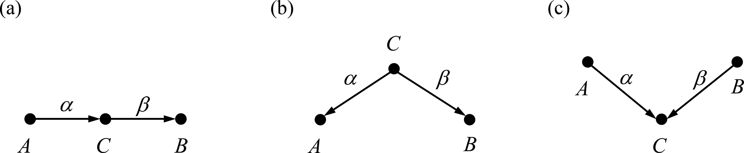
Basic causal structures consisting of three variables. (a) C plays a mediating role between A and B. (b) C is a common cause of A and B. (c) C is a common outcome of A and B.
Causal structures encode statistical (in)dependences among variables (Pearl, 1988). For example, in the two causal structures in Figures 1a and 1b, the variables A and B are not independent of each other (i.e., A and B are marginally associated), and we symbolize this as
d-separation
d-separation is a formal but intuitively understandable rule to extract (conditional) (in)dependence statements from causal structures (Pearl, 2009). A key concept for d-separation is a path in the causal structure. A path is a sequence of connected variables that appear only once regardless of the arrows’ directions. A path can be unconditionally or conditionally blocked or unblocked (i.e., open) by middle variables in the path. In Figure 1a, we find a sole path between A and B: A → C → B. This path is unconditionally open and transmits the association between A and B. This also holds in Figure 1b where the sole path is A ← C → B. However, when a common outcome exists in a path, as in Figure 1c, the path is unconditionally blocked at the common outcome and does not transmit any association. Such common outcomes are often referred to as colliders (Elwert & Winship, 2014). In Figure 1c, the variable C belongs to colliders, and thus, the path A → C ← B is unconditionally blocked at the node C. This path, however, becomes open if the collider variable is conditioned on. That is, conditional on the collider C, the path A → C ← B becomes open and the association is transmitted via the path. 2 If non-collider variables are conditioned on, the path is blocked at the conditioned non-collider variable. As the variable C is not a collider in Figures 1a and 1b, conditional on C, each path is blocked at the node C.
According to d-separation, for a pair of variables, if every path between the pair is blocked by a set of conditioning middle variables (including an empty set), the pair is d-separated by those variables, and then the pair is statistically independent of each other (
Wright’s path-tracing rules
Throughout this article, we restrict our discussion to linear models. Also, for simplicity but without loss of generality, we assume that every variable is normalized to have zero means and unit variances. In standardized linear models, the quantity of the linear relation between a pair of variables can be easily computed by path-tracing rules (Wright, 1921). Given a causal structure, the covariance or correlation—which are identical with standardized variables—between any pair of variables is determined by the sum of products of structural path coefficients along all open paths between the pair (Pearl, 2013). In Figure 1, the Greek letters above the arrows indicate such structural path coefficients. In Figures 1a and 1b, the correlation coefficient between A and B is simply
Discovering Causal Structures of Suppressor Variables
Causal Structures of Classical Suppressors
Horst (1966) provided an example of what is now known as “classical” suppression in which the correlation between the suppressor variable and the criterion is zero. He found that even though there is almost zero correlation between pilots’ verbal ability and their navigational skill, if verbal ability (which is positively correlated with technical ability
3
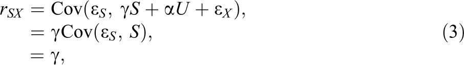
) is included in the regression model, the predictive power of the model (i.e., R2) substantially increases. He claimed that pilots’ verbal ability plays a role as a suppressor in predicting navigational skill with technical ability. That is, verbal ability suppresses some irrelevant variation in the predictor (i.e., technical ability) and thus strengthens the relationship between the predictor and the criterion (i.e., navigational skill). Let X, S, and Y denote the predictor, suppressor, and criterion variables, respectively. Then, the key elements of the example can be expressed with the following three (in)dependence statements:
One can infer the underlying causal structure behind the observed (in)dependence statements. Such inference procedures are known as causal discovery algorithms (see Pearl, 2009, or Spirtes, Glymour, & Scheines, 2000, for details). Our goal is to find a causal structure which is compatible with all three (in)dependence statements. Throughout this article, we assume that the predictor X and the suppressor S precede the criterion variable Y in time. This time ordering is typical in many prediction tasks. Using this background knowledge, we efficiently restrict the causal structure space we have to explore.
The first dependence statement
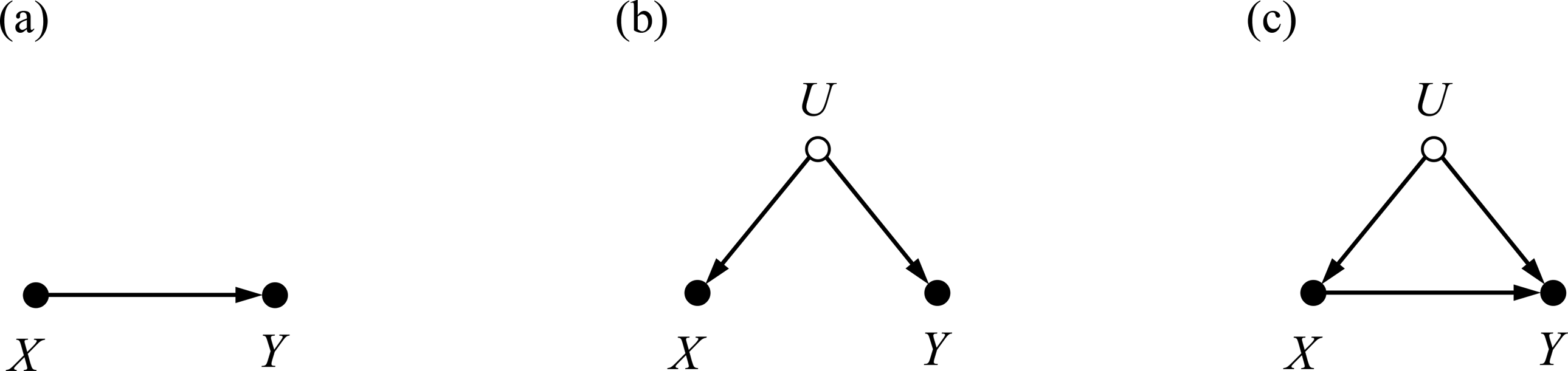
Causal structures creating unconditional dependence between X and Y. (a) X causally affects Y. (b) X and Y are causally affected by an unknown—indicated by a hollow node—common cause U. (c) X and Y are associated via both causal and noncausal relations.
Let us consider the second dependence statement
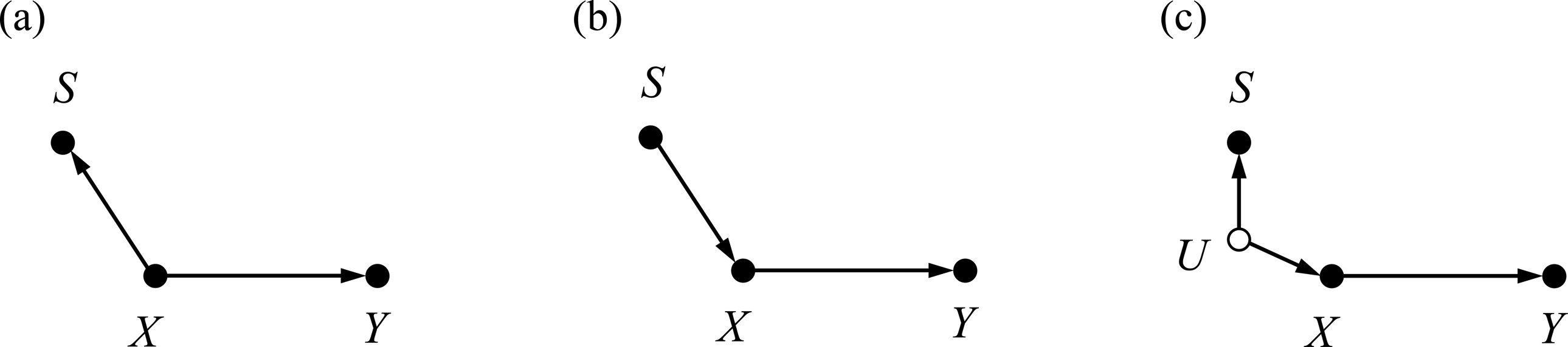
Causal structures encoding two dependence statements
Finally, we now consider the third independence statement between S and Y,
Therefore, we conjecture that the predictor X and the outcome Y are associated only via confounding, as in Figure 2b. Taking this as the basic structure, the possible causal structures embracing the second dependence
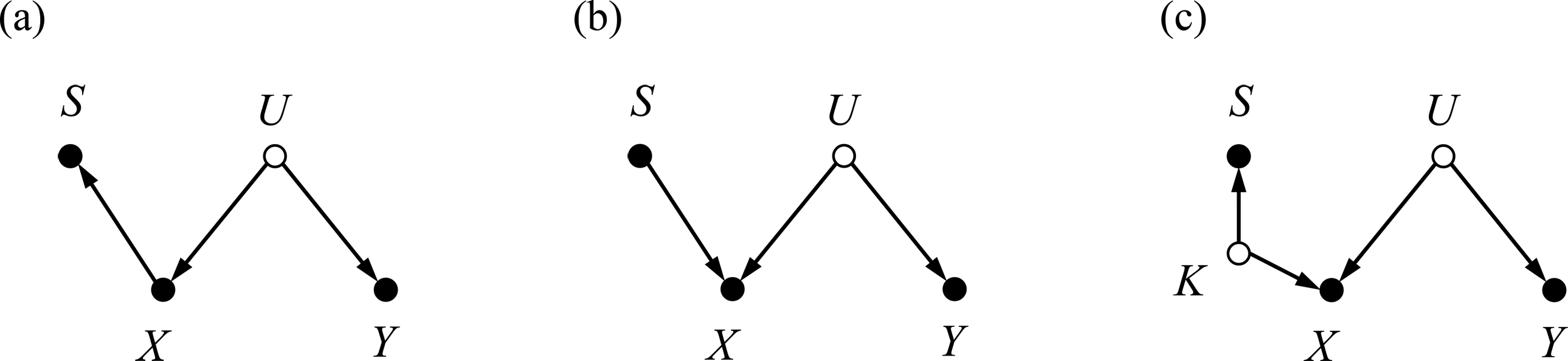
Causal structures encoding two dependence statements
Suppression in Linear Regression Models
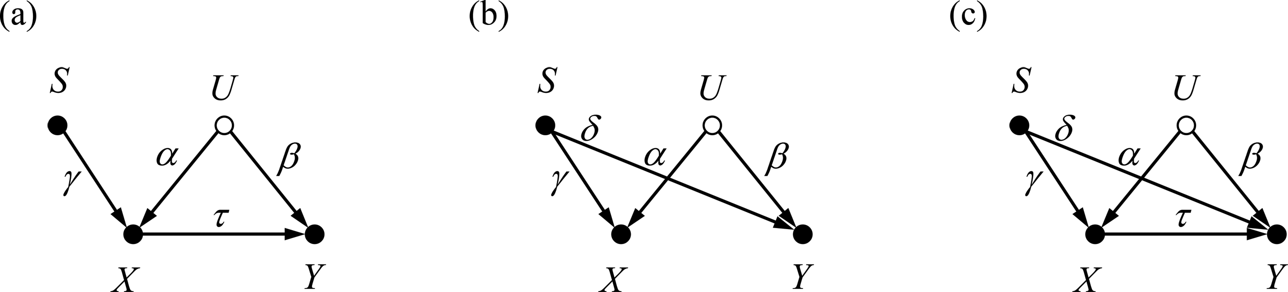
The causal structures we discovered allow us to better understand suppression in linear regression models. For ease of exposition, hereafter, we consider that Figure 4b represents the true causal structure behind Horst’s (1941, 1966) classical suppression, but all the main arguments also hold with Figure 4c. We can write the linear structural causal model corresponding to the causal structure in Figure 4b as
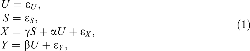
where
Using the data generating model in Equation 1, we now replicate Horst’s (1966) correlation and regression findings in an algebraic manner. First, he found a positive correlation between technical ability (predictor X) and navigational skill (criterion Y). Given Equation 1, the population correlation coefficient between X and Y,
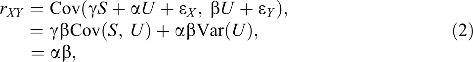
because
because
A noticeable finding was the zero correlation between verbal ability (suppressor S) and navigational skill (criterion Y). Given the structural causal model in Equation 1, the population correlation coefficient between S and Y is
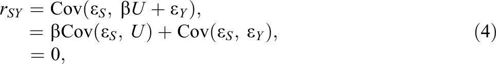
because
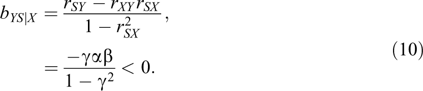
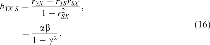
Nonetheless, Horst (1966) found that the partial regression coefficient of verbal ability (suppressor) of the regression of navigational skill (criterion) on technical ability (predictor) and verbal ability was negative, which is the opposite to the positive correlation between verbal ability and navigational skill. The population standardized partial regression coefficient of S after controlling for X is given by 7
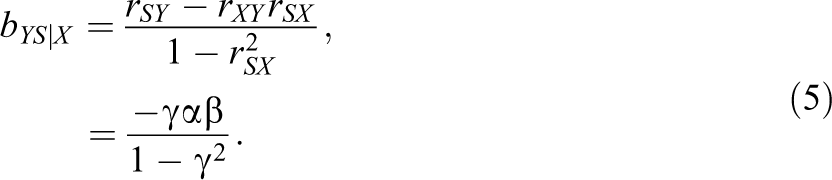
It is obvious that the partial regression coefficient is negative because we already know
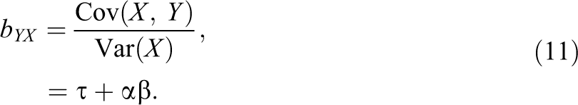
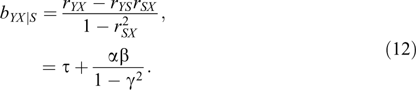
A suppression phenomenon means two increasing or strengthening patterns after controlling for suppressor variables. First, the relationship between the predictor X and the criterion Y should be strengthened by adding the suppressor S into the regression model. The regression coefficient of X of regressing Y on X (without the suppressor S) is
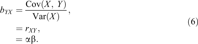
The partial regression coefficient of X of regressing Y on X and S is
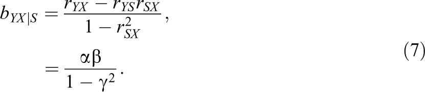
Thus, we see that the inclusion of the suppressor S always amplifies the original relationship between the predictor X and the criterion Y. The classical suppression can be expressed by the inequality
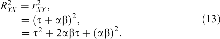
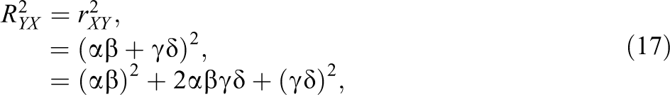
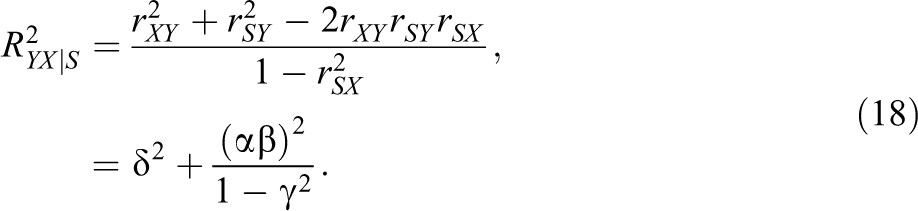
Second, because of the amplification of regression coefficients, suppressor variables substantially increase the predictive power of the regression model. The R2 of the regression model of Y on X (without S) is
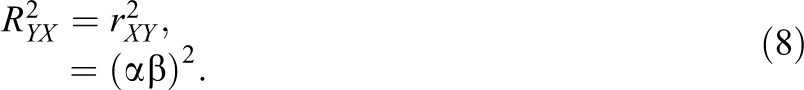
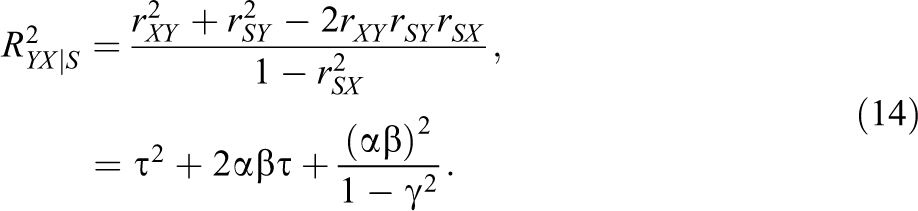
If the suppressor S is added to the regression model, the R2 of the regression model becomes
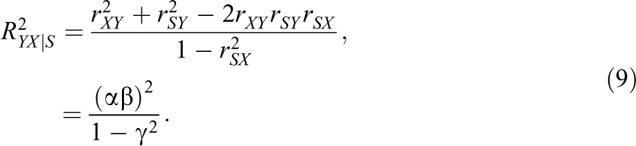
Thus, we see that the original R2 (without S) is again amplified as a result of adding the suppressor S. A comparison of Equations 8 and 9—as well as of Equations 6 and 7—shows that suppression becomes stronger as the structural path coefficient
Causal Structures of Negative Suppressors
After Horst (1941) provided the rationale of classical suppressors, Lubin (1957) asked, “Can a variable act as a suppressor even if it has positive [instead of zero] validity?” (p. 291). Here, the term “validity” indicates the correlation with criterion. Obviously, the causal structure of classical suppressors in Figure 4b (and Figure 4c) does not allow a positive (or more generally, any nonzero) correlation between S and Y. However, Lubin (1957) as well as Darlington (1968) argued that suppression still occurs even when S is positively associated with Y. They referred to such suppressors as negative suppressors.
However, besides the two dependence statements
Causal structures allowing nonzero correlation between S and Y, based on Figure 4b. (a) X causally affects Y. (b) S causally affects Y. (c) X and S causally affect Y. The causal structure in (a) always makes suppression regardless of parameter values.
So, we replicated Lubin’s (1957) setting for negative suppression.
We now investigate whether suppression still occurs with the variable S, which is now positively correlated with Y in Figure 5a. First, the regression coefficient of X on Y (without S) is
If suppression occurs, the relationship between X and Y in Equation 11 should be amplified after controlling for S. The partial regression coefficient of X, controlling for S, is given by
Thus, suppression (i.e., amplifying the association) still occurs because
The same is true for the R2. Without the suppressor S, the R2 of the regression model (i.e., regressing Y on X) is
If the suppressor S is added to the regression model, the R2 is
Since
However, this does not hold in Figures 5b and 5c. In Figure 5b, we have

and the partial regression coefficient for X, controlling for S, as
Now, the inequality is no longer obvious. Depending on
and
Thus, the mechanism of the increase of R2 after including S into the regression model is no longer only due to the amplification (i.e., dividing by
Instrumental Variables in the Causal Inference Literature
Equivalence Between Suppressors and Instrumental Variables
We are interested in now switching our concern from prediction (i.e., predicting pilots’ navigational skill using their technical and verbal abilities) to causal inference (i.e., whether technical ability causally affects navigational skill). Many causal inference researchers probably find an instrumental variable from the causal structures in Figures 4b, 4c, and 5a. An instrumental variable, or simply instrument, is a variable that is related to the treatment but is unrelated to the outcome, except via the treatment. Formally, given a causal structure, a variable S is an instrument with respect to the causal effect of the treatment X on the outcome Y if the following two conditions are met (Pearl, 2009; also see Brito & Pearl, 2002):
9
S is d-connected with X in the causal structure; S is d-separated from Y in the modified structure where the arrow X → Y is deleted.
In Figures 4b, 4c, and 5a, if one considers the predictor X as a treatment variable and the criterion Y as an outcome variable, the suppressor S satisfies the two conditions; therefore, it serves as an instrument. Hence, classical suppressors depicted in Figures 4b and 4c and negative suppressors depicted in Figure 5a are structurally equivalent to instrumental variables.
Despite this equivalence, however, the reasons why instrumental variables are special in the context of causal inference are completely different from the reasons given in support of the use of suppressors in the educational and psychological measurement literature. Suppressors help to amplify the R2 of the regression model which results in a better prediction of the criterion variable. For example, in Horst’s (1966) example, if an evaluator knows a pilot’s verbal ability (suppressor) as well as the pilot’s technical ability (predictor), this evaluator can predict the pilot’s navigational skill (criterion) more accurately. Similarly, educational and psychological researchers have been interested in predicting social behaviors with personality or vice versa. However, this passive prediction is not a major concern in causal inference. Causal inference researchers investigate how a variable (called a treatment) causally affects the other variable (called an outcome). This is not a prediction but a causal explanation.
Identifying Causal Effects With Instrumental Variables
Note that Figure 5a represents a case where the relationship between the treatment X and outcome Y is confounded by the unknown variable U. Then, the causal effect of X on Y cannot be directly obtained from a simple regression analysis of Y on X because of the unmeasured confounding due to U (backdoor criterion; Pearl, 2009). The resulting effect estimate is always biased. In fact, we already witnessed this. The regression coefficient of X in the simple regression model of Y on X in Equation 11 was
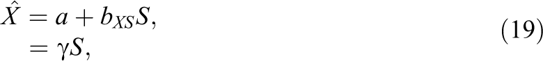
In this case, researchers may use instrumental variables in a very special way for making a causal explanation of X on Y. The two-stage least squares (2SLS) consist of two stages. In the first stage, a researcher regresses the treatment X on the instrument S and obtains the predicted value of the regression model. The regression model is expressed as
because
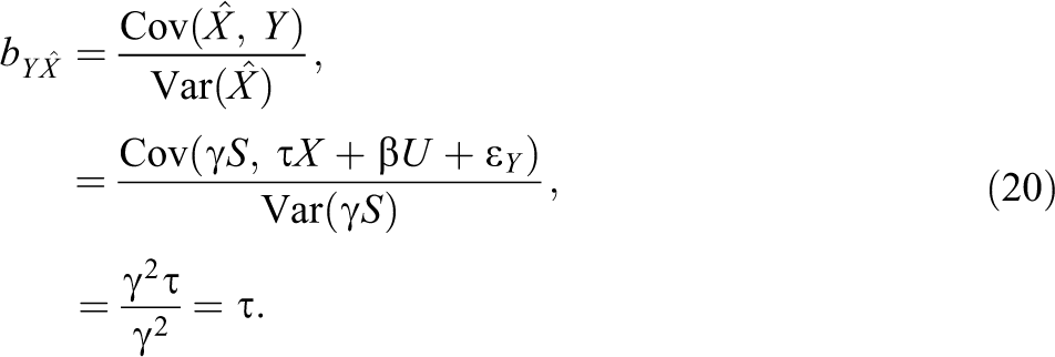
Therefore, even in the presence of an unmeasured confounding due to U, one can correctly identify the causal effect of X on Y using the instrument S. Due to the linearity, the causal identification using instruments is simple here. For the nonparametric identification using instruments, see Angrist, Imbens, and Rubin (1996) or Steiner, Kim, Hall, and Su (2017).
Bias Amplification Due to Instrumental Variables
Note that the 2SLS above is a very special way to use instrumental variables. A group of causal inference researchers recently started looking at consequences of simply controlling for instrumental variables instead of 2SLS (Middleton, Scott, Diakow, & Hill, 2016; Myers et al., 2011; Pearl, 2010, 2011; Steiner & Kim, 2016; Wooldridge, 2009). They have argued that conditioning on instrumental variables is harmful because doing so amplifies any remaining hidden bias. Pearl (2010) referred to this phenomenon as bias amplification. Indeed, we have already witnessed this. Given the causal structure in Figure 5a, the partial regression coefficient for X when regressing Y on both X and S in Equation 12 represents the causal effect estimate of X on Y after controlling for S. It was given by
Illustration
We illustrate our findings using a real data set. Paulhus, Robins, Trzesniewski, and Tracy (2004) provided real examples of suppression in personality research. They investigated the relationship between antisocial behavior and two types of self-esteem, genuine self-esteem and narcissistic self-esteem. Analyzing three independent samples with multiple regression, they argued that both types of self-esteem play a role as a (mutual) suppressor in predicting antisocial behavior. We apply causal discovery algorithms to discover the underlying causal structures behind their data sets. For this illustration, we use TETRAD, a freeware software program developed by Clark Glymour, Richard Scheines, Peter Spirtes, and Joseph Ramsey. 10 Including the PC algorithm (Spirtes & Glymour, 1991), which is a refined version of the IC algorithm we mentioned earlier, TETRAD provides more than 30 different causal search algorithms. Out of those search algorithms, we particularly use the FCI algorithm which allows causal discovery with hidden variables. In Table 1, we present the correlation matrices from Paulhus et al.’s (2004) three samples. 11 Assuming linear models with a normal probability distribution, TETRAD tests the conditional independences between variables and explores underlying causal structures behind these empirical data. 12
Bivariate Correlation Among Two Types of Self-Esteem and Antisocial Behavior in Paulhus et al. (2004)
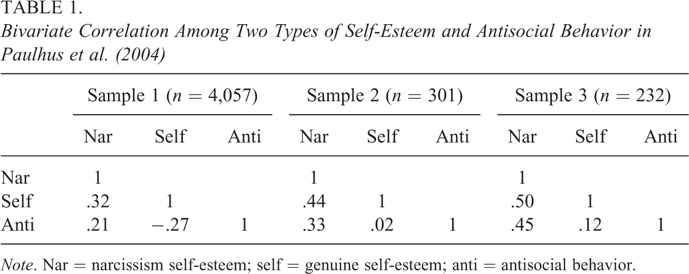
Note. Nar = narcissism self-esteem; self = genuine self-esteem; anti = antisocial behavior.
The causal search results are presented in Figure 6. We found different causal structures from their data. From their Sample 1, the structure depicted in Figure 6a is found. TETRAD uses the edge type, Ao−oB, to indicate that (1) A causes B, or (2) B causes A, or (3) a hidden variable causes both A and B. Thus, we do not have useful information about the underlying causal structure from Sample 1. This is because all variables are correlated with each other. In Table 1, Sample 1 shows a significantly stronger correlation between genuine self-esteem and antisocial behavior (
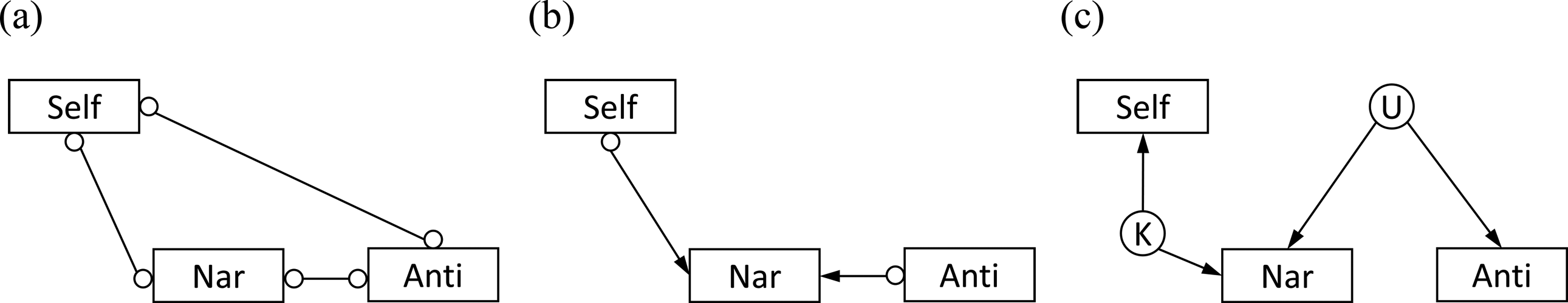
Discovered causal structures from Paulhus et al.’s (2004) self-esteem data sets. (a) Discovered structure from their Sample 1. (b) Discovered structure from their Samples 2 and 3. (c) Modified structure with hidden variables from the graph (b). Nar = narcissistic self-esteem; self = genuine self-esteem; anti = antisocial behavior; K & U = two hidden variables. The edge type, Ao−oB, indicates that (1) A causes B, or (2) B causes A, or (3) a hidden variable causes both A and B. The edge type Ao→B, indicates that (1) A causes B or (2) a hidden variable causes both A and B.
However, both Sample 2 and Sample 3 reveal an informative causal structure depicted in Figure 6b. The edge type, Ao→B, indicates that (1) A causes B or (2) a hidden variable causes both A and B, which would rule out the possibility of B causing A. We find that there are no causal relationships between either type of self-esteem and antisocial behavior from Sample 2 and Sample 3. Relying on the time ordering, one may further restrict the possible causal structures. First, as we have assumed, the regressors, two types of self-esteem, precede in time the criterion antisocial behavior. Second, the two types of self-esteem do not causally affect each other (probably because they are measured almost at the same time). Then, we can infer that two types of self-esteem are associated due to the unknown hidden variable K, and narcissistic self-esteem and antisocial behavior are associated due to another unknown hidden variable U as in Figure 6c.
Note that the structure in Figure 6c is equivalent to the structure in Figure 4c, which is the causal structure of Horst’s (1941, 1966) classical suppression. In Paulhus et al.’s (2004) Samples 2 and 3, genuine self-esteem (“self”) plays the role of a classical suppressor and instrumental variable. Although genuine self-esteem itself has no causal effect on antisocial behavior, the inclusion of it into the regression model of antisocial behavior on both types of self-esteem will suppress some irrelevant variation in narcissistic self-esteem and thus will strengthen the relationship between narcissistic self-esteem and antisocial behavior. This is desirable in terms of making predictions (the R2 change by including genuine self-esteem were, for Sample 2,
Discussion
Over the past 70 years, educational and psychological researchers have viewed suppression effects within a purely statistical framework. Although they succeed to clarify algebraic features of suppression, its interpretation is unclear in the literature. For example, Darlington (1968) wrote: The relations possible among sets of variables are so complex that when a variable with a positive correlation with the criterion variable receives a negative weight in a regression equation, it is generally very difficult or impossible to determine, from the content of the variables, whether the negative weight is “unreasonable.” (p. 179, emphases added)
Importantly, our causal structures of suppressors in Figures 4b, 4c, and 5a reveal that they are indeed equivalent to instrumental variables. Therefore, suppression and bias amplification are also identical phenomena. Despite the long discussion on suppression and instrumental variables, no literature has yet discovered this structural equivalence. In the causal inference literature, the bias amplification has been considered a danger because it will amplify the original confounding bias, which is not desirable from a causal inference perspective (Middleton et al., 2016; Pearl, 2010, 2011; Steiner & Kim, 2016). However, one may interpret this amplifying phenomenon as an enhancement of the relationship between the predictor and the criterion, which can be desirable to better predict the criterion variable. This has been the standard interpretation of suppression in the educational and psychological measurement literature (e.g., Horst, 1941, 1966; Lubin, 1957; Maassen & Bakker, 2001; MacKinnon et al., 2000; Pandey & Elliott, 2010; Shieh, 2006). The two disciplines have focused on different purposes of statistical models and thus have interpreted the same phenomenon from a completely opposite point of view.
Our findings have implications for variable selection in regression, propensity score, or missing imputation models. In addition to utilizing conventional variable selection methods like stepwise selection, recent researchers have started looking at various techniques to select variables such as random forests (Genuer, Poggi, & Tuleau-Malot, 2010), neural networks (Keller, Kim, & Steiner, 2015), or tests of conditional independence (de Luna, Waernbaum, & Richardson, 2011; VanderWeele & Shpitser, 2011). Importantly, however, “[t]he criteria for choosing variables differ markedly in [causal] explanatory versus predictive contexts” (Shmueli, 2010, p. 297; see also Hernán & Robins, 2017). Thus, Genuer, Poggi, and Tuleau-Malot (2010) proposed separate variable selection procedures using random forests for each of causal inference and prediction (see also Shortreed & Ertefaie, 2017, using lasso). Suppressors and instruments serve as a nice example of the importance of clarifying such purposes for variable selection. If one’s goal is to make an accurate prediction, suppressors should be included because doing so amplifies the power of the models to predict the criterion variable. In contrast, if one’s goal is to derive a valid causal explanation, instruments should be excluded because doing so amplifies any remaining confounding bias in causal effect estimates.
Footnotes
Appendix
Acknowledgments
The author thanks Nick Brown, Felix Elwert, Peter Steiner, Jee-Seon Kim, and Eunjin Seo for their helpful comments.
Declaration of Conflicting Interests
The author(s) declared no potential conflicts of interest with respect to the research, authorship, and/or publication of this article.
Funding
The author(s) received no financial support for the research, authorship, and/or publication of this article