A Scaled Threshold Model for Measuring Extreme Response Style

1. Introduction

Cronbach (1946) observed that responses to questionnaire items are affected by individual response styles influencing the response patterns independently from item content. One well-known response style, the so-called extreme response style (ERS), denotes the tendency of an individual to prefer the outer response categories, thus using the rating scale as if it were dichotomous (e.g., Greenleaf, 1992). Relevance and impact of ERS regarding the objectivity and validity of questionnaire data have been verified repeatedly (e.g., Baumgartner & Steenkamp, 2001; De Jong, Steenkamp, Fox, & Baumgartner, 2008; Khorramdel & von Davier, 2014; Naemi, Beal, & Payne, 2009; Weijters, Schillewaert, & Geuens, 2008). Thus, if not accounted for, ERS is likely to compromise results of studies analyzing item responses at least to some extent.

In recent years, several latent trait models have been introduced accounting for ERS in ordered categorical responses. Essentially, there are two main modeling approaches, although models within these approaches are rather heterogeneous themselves. The first approach, which will not be considered further in this article, uses a dichotomous conceptualization of ERS. Specifically, a dichotomous indicator variable, indicating whether an extreme response category was selected or not, is used to measure ERS (e.g., Böckenholt, 2012; Khorramdel & von Davier, 2014; Plieninger & Meiser, 2014). The second approach, which is considered in detail in the following, models ERS by modifying the spacing between responses for each responder individually. Individuals having a decreased spacing between responses assign their responses within a limited range, whereas responders with an increased spacing are more likely to select the extreme response categories. In contrast to the first approach, an extreme response is considered as a consequence of an increased spacing rather than the exclusive preference for the outer versus inner categories of a response scale.

Modifying the spacing between responses can be achieved in various ways. One general approach assumes heterogeneous thresholds (e.g., Javaras & Ripley, 2007; Jin & Wang, 2014; Johnson, 2003; Rossi, Gilula, & Allenby, 2001). The term heterogeneous thresholds means that instead of one set of thresholds applying to all responders, an individual set of thresholds is assumed for each responder. In this way, thresholds are adjusted to account for individual ERS.

A parsimonious way to model heterogeneous thresholds is to include an additional latent variable measuring ERS to an established polytomous item response model. This additional variable operates as a responder-specific scaling factor contracting or expanding intervals between thresholds to adjust differences in response spacing for each individual. However, while scaling thresholds is a sensible and useful approach for modeling ERS, this approach cannot be used arbitrarily in connection with any polytomous item response model as previous research on heterogeneous thresholds might have suggested. Instead, it is important to carefully consider the type of category probability logit and also the required constraint on the thresholds if they are modeled in connection with a scaling factor.

The use of a responder-specific scaling factors is not novel and has been used in other forms to model idiosyncratic response behavior. Ferrando (2009) proposed a model for ordered categorical items with responder-specific residual scales, and Lubbe and Schuster (2017) proposed a model that assumes responder-specific factor loadings. These models, although conceptually similar, achieve different purposes when compared to a model with heterogeneous thresholds. Differences between them and the model proposed in this article will be outlined below.

The article is organized as follows. First, we introduce a new model using scaled thresholds. Second, we demonstrate why we consider this new approach of modeling scaled thresholds as superior by contrasting it to other previously proposed model specifications. Third, we compare the present model to other types of scaling factor models, specifically those of Ferrando (2009) and Lubbe and Schuster (2017), and point out structural differences. Fourth, we demonstrate the small sample parameter recovery of our model using Monte Carlo simulation. Fifth, we analyze two empirical samples of questionnaire responses. Finally, results are summarized and discussed.

2. The Scaled Threshold Model (STM)

In the following, a model is considered that uses a responder-specific scaling factor accounting for ERS on the basis of the graded response model (GRM; Samejima, 1969). According to the GRM, the probability for individual i to select for q-categorical item j response category k is

P ( y i j = k | θ i ) = F ( a j [ θ i − κ j ( k − 1 ) ] ) − F ( a j [ θ i − κ j k ] ) ,

1

where F ( x ) = e x / ( 1 + e x ) , θ _i is the trait, a_j is an item discrimination parameter, and κ j k are thresholds, with − ∞ = κ j 0 < κ j 1 < . . . < κ j ( q − 1 ) < κ j q = ∞ .

For modeling ERS, thresholds parameters κ j k are replaced by sets of responder-specific thresholds κ i j k . In this case,

P ( y i j = k | θ i ) = F ( a j [ θ i − κ i j ( k − 1 ) ] ) − F ( a j [ θ i − κ i j k ] ) ,

2

where κ i j k are

κ i j k = β j + ω i δ j k .

3

In this decomposition of the κ i j k parameters, ω _i is a latent variable measuring ERS, β _j is a scale midpoint parameter, and δ j k are the thresholds’ deviations from β _j , defined by the equation κ j k = β j + δ j k , with − ∞ = δ j 0 < δ j 1 < . . . < δ j ( q − 1 ) < δ j q = ∞ . Note that the δ j k parameters need to satisfy one constraint for their identification. For this purpose, we fix the median of δ j k to zero for each item. The rationale behind this constraint will be explained below. We refer to the new model as STM.

The distributional assumptions for the latent variables are

( θ i log ( ω i ) ) ∼ N [ ( 0 − σ ω 2 / 2 ) , ( 1 0 0 σ ω 2 ) ] .

It follows that ω _i is log-normally distributed having an expected value of 1.0 and a variance of e x p ( σ ω 2 ) − 1 . The log-normal distribution is a standard assumption for scaling factors, which are restricted to the positive real numbers.

Responder-specific thresholds ( κ i j k ) in Equation 3 are obtained by scaling item-specific threshold deviations ( δ j k ) using a responder-specific latent variable (ω _i ). Because κ i j k are obtained with the help of a scaling factor, we refer to them as scaled thresholds.

It is natural to consider extreme responders and midpoint responders as opposite extremes of the same continuum. For defining the extremes of scaling factor (ω _i ) accordingly, the positioning of the β parameters is important. Specifically, β _j needs to be placed in the location that corresponds to the center of the response scale as it is perceived by the responder. Only then will responses converge toward the middle categories as ω _i increases and will be shifted away from the scale middle toward the extreme response categories as ω _i decreases.

Positioning β _j in the response scale’s perceived middle is achieved by fixing the median of threshold deviations δ j k to zero. Note that this median constraint operates differently depending on whether the number of response categories is odd or even. In case of an even number of response categories, the deviation of the middle threshold from midpoint parameter (β _j ) is fixed to zero, that is, δ j ( q / 2 ) = 0 . It follows that in this case, β j = κ i j ( q / 2 ) . Thus, β _j is positioned at the middle threshold, which is identical for all responders irrespective of their scaling factor value. In case of an odd number of response categories, the sum of threshold deviations pertaining to the thresholds surrounding the middle category is fixed to zero, that is, 0 = δ j [ ( q − 1 ) / 2 ] + δ j [ ( q + 1 ) / 2 ] . Therefore, β _j is positioned at the center of the middle category, that is, between thresholds κ i j [ ( q − 1 ) / 2 ] and κ i j [ ( q + 1 ) / 2 ] .

To illustrate the manner in which scaled thresholds account for different response styles, consider a four-categorical scale with labels strongly disagree, disagree, agree, and strongly agree. In this case, β _j characterizes the middle threshold, that is, the threshold between categories disagree and agree. Figure 1 gives the category characteristic curves (CCCs) of responders with three different scaling factors and the same arbitrary trait (θ) for a four-categorical item (j). Item parameters are a j = 1 , β j = 1 , δ j 1 = − 1.0 , and δ j 3 = 1.5 . The second threshold deviation is fixed to zero. The scaling factor values, together with the related scaled thresholds, are ω 1 = 2.0 ( κ 1 j 1 = − 1.0 , κ 1 j 2 = 1.0 , and κ 1 j 3 = 4.0 ), ω 2 = 1.0 ( κ 2 j 1 = 0 , κ 2 j 2 = 1.0 , and κ 2 j 3 = 2.5 ), and ω 3 = 0.5 ( κ 3 j 1 = 0.5 κ 3 j 2 = 1.0 , and κ 3 j 3 = 1.75 ).

OPEN IN VIEWER

Figure 1.

Category characteristic curves of the jth item assuming three responder-specific scaling factors. The plots show how the thresholds are pulled toward the perceived middle β j as ω_i decreases. Note that because q = 4 , β j = κ ij 2 , for i = 1 , 2 , 3 .

The first scaling factor value of ω 1 = 2.0 characterizes a midpoint responder. For this responder, scaled threshold is shifted away from the scale middle. As a consequence, the probability of selecting middle categories, labeled disagree and agree, is increased compared to responders with smaller ω values. Clearly, if β _j were not positioned in the response scale’s middle, increasing ω values would not necessarily result in an increased preference for the middle categories. The second value of ω 2 = 1.0 characterizes an average responder, for whom thresholds are neither contracted nor expanded by ω. Finally, a responder with ω 3 = 0.5 is an extreme responder. His thresholds are contracted toward scale midpoint parameter (β _j ). Consequently, the probability of selecting extreme categories strongly disagree and strongly agree is increased considerably.

For a response scale with an odd number of categories, the principle is equivalent. As an example consider a five-categorical response scale with response labels strongly disagree, disagree, neutral, agree, and strongly agree. For this scale, the β parameter is positioned in the middle of the neutral category. Again, responders with small scaling factor values prefer the extreme response categories, whereas responders with large ω values prefer the neutral category.

3. Alternative Model Specifications

In the following, we contrast the current model specifications to potential modifications that might seem natural but will limit the model’s capability to account for ERS. Specifically, we consider modifying the threshold constraint and the type of category probability logit. These modifications are of particular relevance because they have been used previously for scaling factor models.

3.1. Threshold Constraint

The median constraint on threshold deviations ( δ j k ) is rather unusual. More common is the so-called sum constraint that fixes their sum per item to zero. The sum constraint is used, for instance, in the rating scale model (Andrich, 1978). Because for most polytomous item response models, it is arbitrary whether the sum, median, or any individual parameter is fixed to zero, the importance of selecting a specific constraint has not drawn much attention previously. However, using a sum constraint for modeling ERS with scaled thresholds is indeed problematic.

As was outlined, by positioning β _j in the response scale’s perceived middle, extreme and midpoint responders are defined as opposite extremes on the ω continuum. More specifically, only in this case will the probability of selecting a middle category consistently increase as ω _i increases. To ensure that β _j is always positioned in the response scale’s middle, the median constraint on threshold deviations δ j k is the only viable option. A sum constraint, on the other hand, does not achieve the same purpose.

To illustrate, let’s consider a set of thresholds pertaining to a five-categorical response scale. Specifically, we assume thresholds of κ j 1 = − 2.0 , κ j 2 = 1.5 , κ j 3 = 2.5 , and κ j 4 = 3.0 . Clearly, the value of β _j differs depending on the selected constraint for the threshold deviations. If the median constraint is used, then the value of β _j is 2.0, lying directly between the second and third threshold, which is the perceived middle of the scale. If, however, the sum constrained is applied, then β j = 1.25 , which is a value centered within the disagree category. Figure 2 displays the position of β _j in relation to the response categories of the five-categorical response scale for both types of constraints.

OPEN IN VIEWER

Figure 2.

β parameter positions of a five-categorical scale for median and sum constrained threshold deviations.

If the median constraint is used, β _j lies between both thresholds surrounding the neutral category. If, however, the sum constraint is applied, β _j lies in the disagree category. While the different threshold deviation constraints are of little consequence for responders with average ω values, it becomes relevant for responders with large ω values, who are considered midpoint responders. Increasing the probability of selecting the middle category can be achieved by expanding the interval between the thresholds surrounding it. In connection with our example, this means shifting the second and third threshold farther away from each other. Obviously, this is achieved best if β _j is positioned within the middle category. However, if β _j lies outside of the middle category, a different result is obtained. Specifically, for large values of ω, the probability of selecting the disagree category approaches 1.0 for the present example if the sum constraint is used. Clearly, this appears to be an undesirable model property.

3.2. Category Probability Logit

The type of category probability logit used in connection with scaled thresholds needs to be considered carefully. Two commonly used types of logits when modeling ordered categorical data are the adjacent category logit and the cumulative logit (e.g., Agresti, 2003).

The adjacent category logit considers the probabilities of two consecutive categories k and k + 1 , that is

log [ P ( y = k + 1 ) P ( y = k ) ] , for k = 1 , . . . , q − 1.

It is commonly used in connection with Rasch rating models such as the rating scale model (Andrich, 1978), the partial credit model (Masters, 1982), or the generalized partial credit model (Muraki, 1992).

The cumulative logit considers the probability of selecting any category higher than the kth category versus the remaining categories, that is

log [ P ( y = k + 1 ) + . . . + P ( y = q ) P ( y = 1 ) + . . . + P ( y = k ) ] , for k = 1 , . . . , q − 1.

A well-known model using this logit is the GRM (Samejima, 1969).

In latent variable models, thresholds characterize the locations where the category probability logits are zero on the latent trait continuum, that is, where the logit’s numerator and denominator probabilities are identical. Thus, for models with adjacent category logits, thresholds mark the transition between adjacent categories, which equals the trait for which either of two consecutive categories is selected with the same probability. For models with cumulative logits, thresholds separate regions of a continuum corresponding to the ordered response categories, that is, the point where either of both regions is selected with probabilities of .5 (e.g., Masters, 1982). It follows that if thresholds based on either logit differ, then scaling factors that modify them will operate differently as well.

While our model uses cumulative logits, the model of Jin and Wang (2014) uses adjacent category logits. Their model can be expressed in terms of the logit of the probabilities of two consecutive response categories (see their equation 10), that is

log [ P ( y i j = k + 1 ) P ( y i j = k ) ] = θ i − ( μ j + ω i τ j k ) ,

4

where θ _i is the trait, μ _j is an item difficulty parameter, and τ j k are threshold parameters satisfying a sum constraint. Although the interpretation of μ _j and τ j k is closely related to those of β _j and δ j k of the STM, they are different parameters. However, for a concise presentation, we will use the symbols of the STM. Specifically, in the following, we will use β _j instead of μ _j and δ j k instead of τ j k when considering a model with adjacent category logits.

Before we compare both logit types for modeling ERS with scaled thresholds, note that, in general, adjacent category logits are by no means inferior to cumulative logits. Indeed, in some cases, they are more flexible because they are not restricted to modeling ordered response categories but can be applied to nominal data also. However, in the present context, their flexibility introduces unnecessary complexity. Indeed, depending on the specific model parameters, scaling factors modeled in connection with adjacent category logits do not yield a meaningful interpretation in terms of measuring ERS. This limitation can be explained best by outlining two problematic properties.

First, consider the ordering of thresholds. As is well known, when using cumulative logits, thresholds have to be ordered by definition, that is, κ j 1 < κ j 2 < . . . < κ j ( q − 1 ) . Thresholds of models with adjacent category logits, on the other hand, do not need to be ordered. Indeed, disordered thresholds occur frequently and, therefore, may be considered the rule rather than the exception (e.g., Adams, Wu, & Wilson, 2012; Masters, 1982).

For scaling factor (ω) to unanimously account for ERS across items, thresholds of all items are required to be ordered. Only then will decreasing ω values yield increased probabilities for selecting the outer response categories for all items and vice versa. However, if the order of thresholds differs between items, their scaling with ω yields different results.

To illustrate, consider 2 three-categorical items. Item parameters of the first item are β 1 = 0 , δ 11 = − 1 , and δ 12 = 1 . Item parameters of the second item are β 2 = 0 , δ 21 = 1 , and δ 22 = − 1 , where in contrast to the first item, thresholds are inverted. Figure 3 gives the probability of an extreme response as a function of θ for ω values of 2.0, 1.0, and 0.1 for both items. For Item 1, the probability of an extreme response increases as ω decreases. However, for Item 2, where thresholds are inverted, the probability of an extreme response decreases as ω decreases, that is, the scaling factor now has the opposite effect.

OPEN IN VIEWER

Figure 3.

Probability of an extreme response of the model of adjacent category logits for two exemplary items and three different ω values: ω 1 = 0.1 , dashed ω 2 = 1.0 , dotted ω 3 = 2.0 . Threshold deviations of Item 1 are δ 11 = − 1 and δ 12 = 1 and those of Item 2 are δ 21 = 1 and δ 22 = − 1 . Furthermore, β 1 = β 2 = 0 .

Although this is only one of many conceivable patterns for disordered thresholds, it clearly shows that effect and interpretation of scaling factor ω depend on the thresholds’ order. Obviously, this is an undesirable model property because ω is intended to measure ERS for all items similarly. Models using cumulative logits, on the other hand, do not have this limitation because their thresholds are ordered and, therefore, they yield a unanimous interpretation of the scaling factor.

To illustrate the second problematic property of using adjacent category logits, Figure 4 shows the CCCs of responders with three different scaling factors for a three-categorical item. To emphasize the distinction between middle and outer response categories, the curve of the middle category is printed in bold, whereas dashed lines are used for the curves of the outer response categories. Item parameters are β = 0.0 , δ 1 = − 1.0 , and δ 2 = 1.0 , and values of the scaling factor are ω 1 = 2.0 , ω 2 = 1.0 , and ω 3 = 0.1 . The three plots on the left contain the CCCs of the model using adjacent category logits, and those on the right contain the CCCs of STM with cumulative logits.

OPEN IN VIEWER

Figure 4.

Category characteristic curves of scaled threshold models based on adjacent category and cumulative logits for different ω values. Item parameters are β = 0.0 , δ 1 = − 1.0 , and δ 2 = 1.0 . Dotted vertical lines show scaled thresholds.

Scaled thresholds ( ω i δ k ) of the model with adjacent category logits are at the point where the curves of adjacent categories intersect, that is, where the probability of selecting either of two adjacent categories is identical. Scaled thresholds of the STM are at the point, where the probability of selecting any of the categories below or above it is .5.

The first row of Figure 4 gives the CCCs of a responder with a tendency for preferring the middle category ( ω 1 = 2.0 ). Consequently, the interval between scaled thresholds is large. In this case, CCCs of both models are almost identical. The second row gives CCCs of an average responder ( ω 2 = 1.0 ) who has neither an increased preference for the outer nor inner categories. The third row shows the CCCs of an extreme responder ( ω 3 = 0.1 ). For this person, the interval between both scaled thresholds is small. Clearly, as ω approaches zero, the differences between category probabilities of both models become larger.

As the graphs on the left in Figure 4 pertaining to adjacent category logits show, the probability of an extreme response does not approach 1.0 for all trait levels as the scaling factor approaches zero. Specifically, if θ is close to β, there is still a considerable probability for selecting the middle category, even if ω = 0.0 . For the STM, on the other hand, the probability for selecting the middle category approaches .0 for all trait values.

Clearly, using adjacent category logits in connection with the outlined assumptions fails to fit response patterns of most persistent extreme responders, that is, responders who exclusively use the outer response categories. Not accounting for such response patterns is problematic because they are frequently observed in empirical data (e.g., Bachman & O’Malley, 1984; Baumgartner & Steenkamp, 2001). Using the STM, this is not an issue because as it’s scaling factor ω approaches zero, the probability of selecting the middle category approaches zero, too.

4. Other Scaling Factor Models

To illustrate the unique features of the STM, we compare it to (a) the GRM for measuring person reliability (PRM) of Ferrando (2009) and (b) the graded response differential discrimination model (GRDDM) of Lubbe and Schuster (2017). Similar to the STM, they are both modified versions of the GRM using an additional scaling factor.

The PRM was proposed to account for individual differences in reliability of responses. This is achieved by including a responder-specific scaling factor in the form of a person discrimination parameter. Although this model was not developed as an ERS model, its parameters also account for differential preferences for extreme categories. Specifically, the PRM assumes the following category probability function:

P ( y i j = k | θ i , a i ) = F ( a i ( θ i − κ j ( k − 1 ) ) ) − F ( a i ( θ i − κ j k ) ) ,

where, in contrast to the GRM in Equation 1, the item-specific discrimination parameter a_j has been replaced with a responder-specific discrimination a_i modeling the inverse of the residual standard deviations for each responder. Similar models also including a random residual scale have been proposed by Cleveland, Denby, and Liu (2000) and Hedeker, Mermelstein, Hakan, and Berbaum (2016).

The GRDDM is more closely related to the STM. However, instead of shifting thresholds, it shifts the expected response of an individual toward or away from the scale midpoint using responder-specific discrimination parameter a i j , resulting from the multiplication of item discrimination (a_j) and scaling factor (α _i ), that is, a i j = a j ⋅ α i . The category probability function of the GRDDM is

P ( y i j = k | θ i , α i ) = F ( a i j ( θ i − β j ) − δ j ( k − 1 ) ) − F ( a i j ( θ i − β j ) − δ j k ) .

Similarly to the STM, β _j is defined by the median constraint as an item-specific midpoint parameter, and δ j k are the thresholds’ deviations from β _j . Consequently, if a i j is large, then the expected response is shifted away from the midpoint, and if a i j is small, responses are centered in the scale middle.

The STM cannot be equated with the other two models. Nevertheless, the respective approaches bear obvious similarities. For both PRM and GRDDM, the probability of an extreme response changes depending on the value of the scaling factor. However, the change in extreme response probability is directly linked to discrimination parameters, which, if modeled responder-specific, are also indicators of the reliability of an individual’s response pattern. Similarly to a high item discrimination, a high person discrimination implies that item response and trait correspond more closely to each other than for an individual with a low person discrimination.

The a_i parameter of the PRM may be considered as a responder-specific scale parameter, whereas the a i j parameter of the GRDDM can be regarded as a responder-specific slope parameter. Interestingly, large values in either parameter will yield opposite effects on the probability for selecting an extreme response. For the PRM, extreme responses become more likely as the scaling factor becomes smaller, whereas for the GRDDM, the probability of an extreme response increases as the scaling factor becomes larger. A more detailed comparison between both models can be found in Lubbe and Schuster (2017).

The STM, on the other hand, does not assume any relation between the reliability of a response pattern and the probability of an extreme response. Its scaling factor only affects the thresholds and, therefore, does not alter any parameter associated with response reliability. In this way, the STM exclusively models response spacing by expanding or contracting intervals between response categories.

5. Simulation Study

Consistent parameter estimates for polyomous item response models with scaled thresholds can be obtained by using either Markov chain Monte Carlo methods or a marginal maximum likelihood approach (e.g., Lubbe & Schuster, 2017; Rossi et al., 2001). However, consistent estimation does not necessarily preclude biased parameter estimates in small samples. Thus, in the following, we will investigate the parameter recovery of the STM in small samples using Monte Carlo simulation based on marginal maximum likelihood estimation.

We generated data sets with 8 five-categorical items for samples sizes of n = 150 and 250. The same numbers of items and response categories are, for instance, used for the BIG-5 facets of the frequently applied NEO Personality Inventory–Revised (NEO PI-R; Costa & McCrae, 1992). Item parameters were a j = 1 , with j = 1 , . . . ,8 ; β 1 = − 1 ; β 2 = − 2 / 3 ; β 3 = − 1 / 3 ; β 4 = 0 ; β 5 = 0 ; β 6 = 1 / 3 ; β 7 = 2 / 3 ; β 8 = 1 ; δ j 1 = 2 ; δ j 2 = 0.5 ; δ j 3 = − 0.5 ; and δ j 4 = − 2 . Note that δ j 2 and δ j 3 satisfy the constraint δ j 2 = − δ j 3 . For the scaling factor variance ( σ ω 2 ), we consider three conditions. In one condition, we fixed σ ω 2 to 0.0, examining whether the model correctly rejects any systematic variation of the scaling factor if it does not account for differences in ERS. In addition, we used σ ω 2 values of 0.15 and 0.30. We consider these as realistic parameter values, as supported by the empirical examples below.

For each of the six data constellations, resulting from the combination of sample size and scaling factor variance, we generated 100 samples. Model fitting was performed using SAS PROC NLMIXED with adaptive Gauss-Hermite quadrature using five quadrature points and quasi-Newton optimization. Exemplary SAS PROC NLMIXED code is provided in the Appendix section. Using the default settings for convergence of the NLMIXED procedure, all models reached convergence.

Table 1 gives the average parameter estimates of the STM for the six simulations together with the true parameter values. Clearly, the deviation of the average estimates from the true parameter values is extremely small. Only in case of a sample size of 150, there is a small tendency for β _j and δ j k estimates to be slightly more extreme than their true value. However, this bias still is negligible.

OPEN IN VIEWER

Table 1.

Average STM Estimates Under the Four Simulation Study Conditions

Parameter	n = 150			n = 250			True Value
	σ ω 2 = .0	σ ω 2 = .15	σ ω 2 = .30	σ ω 2 = .0	σ ω 2 = .15	σ ω 2 = .30
σ ω 2	0.008	0.155	0.294	0.005	0.152	0.293	See σ ω 2
aj	1.002	1.032	1.025	0.996	1.005	1.033	1.000
β1	− 1.033	− 1.049	− 1.043	− 1.024	− 1.057	− 1.025	− 1.000
β2	− 0.716	− 0.700	− 0.702	− 0.660	− 0.665	− 0.693	− 0.667
β3	− 0.327	− 0.350	− 0.355	− 0.319	− 0.346	− 0.363	− 0.333
β4	0.013	0.011	− 0.030	− 0.001	− 0.013	0.001	0.000
β5	− 0.003	0.024	0.024	− 0.002	− 0.007	− 0.003	0.000
β6	0.390	0.336	0.346	0.412	0.359	0.320	0.333
β7	0.663	0.702	0.689	0.639	0.676	0.669	0.667
β8	1.037	1.061	1.089	1.029	1.007	0.975	1.000
δ j 1	2.102	2.098	2.115	2.056	2.069	2.005	2.000
δ j 2	0.522	0.527	0.527	0.513	0.512	0.503	0.500
δ j 4	− 2.097	− 2.109	− 2.136	− 2.060	− 2.077	− 2.018	− 2.000

Note. Estimates of δ j 3 are redundant and, therefore, not included because of identification constraint δ j 2 = − δ j 3 . STM = scaled threshold model.

In addition, the reliability of the estimates’ standard errors is of practical relevance. It can be investigated by comparing standard error estimates to the empirical distribution of estimates across data samples. Specifically, if the averaged standard errors and the parameter estimates’ standard deviations across replications are close, this can be considered as evidence for the reliability of the former.

As Table 2 shows, averaged standard errors and the estimates’ standard deviations are almost identical. Only standard errors of δ j 1 and δ j 4 appear to underestimate the sampling error to some minor extent if the sample size is 150. However, this is not unexpected because in these specific conditions, estimates are also slightly biased.

OPEN IN VIEWER

Table 2.

Average Standard Errors and Standard Deviation of Parameter Estimates Under the Four Simulation Study Conditions

Parameter	n = 150			n = 250
	σ ω 2 = .0	σ ω 2 = .15	σ ω 2 = .30	σ ω 2 = .0	σ ω 2 = .15	σ ω 2 = .30
σ ω 2	.018/.012	.037/.037	.055/.054	.014/.008	.029/.031	.042/.046
aj	.252/.213	.255/.258	.262/.278	.193/.137	.194/.186	.199/.203
β1	.297/.252	.310/.354	.313/.328	.216/.169	.231/.209	.228/.237
β2	.254/.237	.241/.244	.248/.252	.181/.147	.178/.189	.186/.184
β3	.197/.149	.204/.217	.214/.200	.153/.136	.156/.156	.153/.166
β4	.188/.181	.193/.204	.197/.210	.145/.123	.147/.151	.142/.136
β5	.192/.163	.192/.195	.205/.187	.144/.114	.147/.137	.146/.132
β6	.219/.212	.209/.225	.211/.212	.169/.150	.162/.186	.152/.158
β7	.240/.252	.243/.214	.245/.230	.174/.203	.180/.190	.180/.164
β8	.291/.226	.310/.307	.325/.287	.222/.179	.219/.187	.211/.183
δ j 1	.516/.478	.539/.577	.578/.626	.377/.292	.397/.406	.391/.404
δ j 2	.141/.127	.144/.145	.150/.157	.104/.094	.105/.104	.104/.102
δ j 4	.517/.471	.540/.570	.583/.616	.377/.288	.399/.401	.395/.391

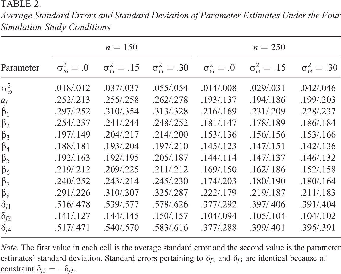
Note. The first value in each cell is the average standard error and the second value is the parameter estimates’ standard deviation. Standard errors pertaining to δ j 2 and δ j 3 are identical because of constraint δ j 2 = − δ j 3 .

Overall, the STM (if estimated using marginal maximum likelihood) performs very well in small samples. Already for samples of 250 observations, parameters are virtually unbiased. However, as for any simulation study, it has to be noted that generalizations of results have to be considered with caution.

6. Empirical Examples

In the following, results of two data examples are given. The first example serves to illustrate how to interpret model results using a data set with a small number of variables. In the second example, the impact of altering the type of logit is demonstrated empirically using a representative sample of questionnaire responses.

6.1. Example 1

In the first example, we analyze a sample of responses of 582 undergraduate students to 5 six-categorical items measuring the attitude toward aphorisms. We fitted STM and GRM to the data, using SAS PROC NLMIXED with marginal maximum likelihood estimation with adaptive Gauss-Hermite quadrature and quasi-Newton optimization. The number of quadrature points was fixed to 5 for all analyses.

Table 3 gives the estimates of item discriminations (a_j), midpoint parameters (β _j ), and scaling factor variance ( σ ω 2 ). Clearly, a_j and β _j estimates are very similar for STM and GRM. However, the σ ω 2 estimate of the STM clearly shows that ERS has a considerable effect on item responses. Furthermore, Akaike’s information criterion (AIC) of the STM is 9,194.5, which is distinctly lower than the GRM’s AIC of 9,367.3, indicating the clearly superior fit of the STM.

OPEN IN VIEWER

Table 3.

STM and GRM Parameter Estimates for the Aphorism Data

	STM	GRM
a 1	1.341 (.153)	1.441 (.145)
a 2	1.167 (.147)	1.097 (.124)
a 3	1.186 (.139)	1.224 (.129)
a 4	1.600 (.180)	1.795 (.181)
a 5	1.350 (.155)	1.432 (.146)
β1	− 0.653 (.099)	− 0.627 (.092)
β2	0.707 (.109)	0.695 (.112)
β3	− 0.074 (.089)	− 0.107 (.086)
β4	− 0.447 (.082)	− 0.417 (.075)
β5	− 1.128 (.125)	− 1.079 (.115)
σ ω 2	0.233 (.032)	—

Note. Standard errors are in parentheses. STM = scaled threshold model; GRM = graded response model.

Next, we consider latent variable predictions of STM and GRM. For this purpose, we calculated ω ˆ and θ ˆ values for each responder using the empirical Bayes approach implemented in SAS PROC NLMIXED, which yields maximum a posteriori latent variable predictions. Table 4 gives the ω ˆ and θ ˆ values of the STM and θ ˆ values of the GRM for five exemplary responders who differ systematically in their ERS together with the raw item responses. Specifically, we selected responders with the minimum and maximum ω ˆ values ( ω ˆ = 0.394 and ω ˆ = 2.007 ), an average responder ( ω ˆ = 1.000 ), as well as responders with less extreme tendencies toward ERS ( ω ˆ = 0.750 ) and toward midpoint responses ( ω ˆ = 1.499 ).

OPEN IN VIEWER

Table 4.

Latent Variable Predictions of ω and θ Together With the Item Responses for Five Exemplary Responders

Subject	STM		GRM
	ω ˆ	θ ˆ	θ ˆ	y 1	y 2	y 3	y 4	y 5
499	0.394 (.137)	− 1.320 (.627)	− 1.874 (.596)	6	1	1	1	1
379	0.750 (.242)	0.501 (.559)	0.541 (.527)	3	4	6	4	6
211	1.000 (.289)	0.308 (.532)	0.265 (.462)	5	2	5	4	5
11	1.499 (.502)	− 1.120 (.530)	− 0.820 (.434)	3	2	3	3	3
152	2.007 (.786)	0.433 (.574)	0.030 (.445)	4	4	4	4	4

Note. Standard errors are in parentheses.

The ω ˆ values reflect the pattern of item response very intuitively. Responder 499, who exclusively selects extreme Categories 1 and 6, has the lowest ω ˆ value, whereas Responder 152 restricts responses to Category 4 and has, therefore, the largest ω ˆ value. Comparing the θ predictions of STM and GRM, trait values differ more strongly for extreme values of ω ˆ . For instance, while the GRM yields a large negative trait value of −1.874 for Responder 499, the STM gives a considerably less extreme value of −1.320 because ERS accounts in part for this unusual response pattern. In addition, for individuals preferring the middle categories (11 and 152), θ predictions are shifted away from zero when compared to the θ predictions of the GRM.

Finally, we consider the relation between ω ˆ values and the number of extreme responses. Figure 5 gives boxplots of ω ˆ for numbers of extreme responses from 0 to 5. Although both variables are highly correlated, having a Spearman correlation of −0.905 ( p < .001 ), they show some distinct features. First, ω ˆ values yield more fine-grained differences between grades of ERS than the number of extreme responses (sometimes used as an indicator of ERS). Furthermore, this additional differentiation is most pronounced for responders who avoided using extreme categories. This result is expected because in contrast to merely considering the number of extreme responses, the STM also accounts for differences in response spacing for nonextreme responders. More specifically, when using the numbers of extreme responses, it cannot be differentiated between individuals who, for instance, use Response Categories 2 through 5 versus individuals who restrict responses to Categories 3 and 4. Instead, the STM will consider the former as more extreme responders.

OPEN IN VIEWER

Figure 5.

Relation between latent variable predictions of ω and number of extreme responses for the aphorism data.

6.2. Example 2

To investigate the impact of the choice of category probability logit when modeling scaled thresholds, we analyzed questionnaire responses of the normative sample of the German version of the NEO PI-R (Ostendorf & Angleitner, 2004). Specifically, we analyzed the six facets pertaining to neuroticism: anxiety (N1), angry hostility (N2), depression (N3), self-consciousness (N4), impulsiveness (N5), and vulnerability (N6). Each facet consists of 8 five-categorical items, with response categories strongly disagree, disagree, neutral, agree and strongly agree. The sample comprises N = 12,003 cases. Negative items were recoded prior to analysis. Analyses were performed with identical specifications as in the previous example.

First, we consider the overall model fit. Table 5 gives the AIC for all six neuroticism facets for the STM with cumulative logits and adjacent category logits, respectively. Clearly, AIC values of the STM with cumulative logits are distinctly lower than for the model with adjacent category logits.

OPEN IN VIEWER

Table 5.

AIC Values of All Neuroticism Facts for Cumulative and Adjacent Category Logit Models

Facet	Cumulative	Adjusted Category
	Logit	Logit
N1	231,023	232,115
N2	246,846	248,007
N3	212,933	213,588
N4	243,142	243,923
N5	242,063	243,195
N6	223,699	224,109

Note. AIC = Akaike’s information criterion.

Next, we consider the impact of disordered thresholds on the scaling factor more closely. Note that all of the neuroticims facets had at least 1 item with disordered thresholds when analyzed with the STM with adjacent category logits. Specifically, the number of items with disordered thresholds were 2, 6, 3, 8, 1, and 2 for facets N1 to N6, respectively. To keep our presentation concise, we selected the neuroticism facet with the largest number of items with disordered thresholds, that is, N4, and the one with the smallest number, that is, N5, for further analyses.

For all items with disordered thresholds, the order of the second and third threshold was inverted, that is, δ j 2 > δ j 3 . This is important information with respect to identifying response patterns for which ω estimates will be more or less affected by the thresholds’ order. Specifically, if the middle thresholds are inverted, it can be expected that scaling factors of responders who prefer the middle categories will deviate more strongly between both models than for responders who prefer extreme categories.

We calculated ω ˆ values for each responder using the empirical Bayes approach implemented in SAS PROC NLMIXED. Figure 6 shows the scatterplots of the log ( ω ) values of the STM with cumulative and adjacent category logits for facets N4 and N5, respectively. Note that we use the logarithm of the ω predictions to obtain more symmetrically distributed values. To distinguish responders who preferred the middle categories from the remaining responders, we used gray instead of black color for the responders who exclusively used Nonextreme Categories 2, 3, and 4.

OPEN IN VIEWER

Figure 6.

Relation between log ( ω ) values of models with adjacent category and cumulative logits for facets N4 and N5. Gray color is used for responders who never used Extreme Categories 1 and 5, black color is used for all other responders.

It is obvious that for N5, which has only 1 item with disordered thresholds, the relation between scaling factors of both models is closer than for facet N4, where all 8 items have disordered thresholds. Specifically, the correlation of scaling factors for N5 is .905 and for N4 it is .781.

The heteroscedastic shape of the left scatterplot in Figure 6, pertaining to N4, can also be explained by inverted thresholds. Clearly, the heterogeneity between scaling factors of both models becomes larger as ω values increase, that is, for responders who tend toward the Middle Categories 2, 3, and 4. This specific pattern results because thresholds between these middle categories are inverted for all items of N4. Indeed, for responders who avoided Extreme Categories 1 and 5 entirely (gray dots), the relation between log ( ω ) values of both models is negative, having a correlation of −.473 based on 3,855 observations.

Finally, we consider the relation between scaling factor values of both facets for the STM with cumulative and adjacent category logit, respectively. Because ERS is considered a stable individual characteristic, scaling factors obtained from different item responses should be significantly correlated. Thus, correlating scaling factors of N4 and N5 within each model may be considered as part of construct validation.

Figure 7 gives the scatterplots of the relation between log ( ω ) values of N4 and N5 for models based on adjacent category and cumulative logits, respectively. For the STM, scaling factors of both facets correspond more closely to each other, having a correlation of .384, than for the model with adjacent category logits, where the correlation is .286. While these correlations appear to be small, we regard values close to .4 as satisfactory, given that the ERS value for each person is assessed based on only 8 items.

OPEN IN VIEWER

Figure 7.

Relation between log (ω) values of facets N4 and N5 models based on adjacent category and cumulative logits, respectively.

In summary, the empirical results confirm the limitations of using adjacent category logits in connection with modeling a responder-specific scaling factor. Specifically, the issue of inverted thresholds is clearly illustrated by the inversion of scaling factor values for responders who preferred nonextreme categories for facet N4. The STM, on the other hand, does not reveal any inconsistencies. Model fit and the validity of scaling factor values are superior across all neuroticism facets.

7. Discussion

The present article investigates an approach for modeling ERS in polytomous item responses using scaled thresholds. Specifically, a model is proposed that modifies the distances between thresholds for each responder by means of a latent scaling factor, allowing for the simultaneous and independent measurement of trait and ERS.

While the use of a scaling factor for modeling idiosyncratic response behavior is not new and has proven useful to make a clear conceptual distinction between response behavior and trait, the model we propose has novel features. First, compared to other related models, the STM yields a scaling factor that exclusively measures responder-specific differences in the extremity of the response pattern independently from other responder-specific attributes such as the reliability of responses.

Furthermore, we illustrate that the properties of modeling scaled thresholds are sensitive to choices of model parametrization, such as the type of category probability logit and the constraint imposed on the thresholds deviation parameters for model identification. As has been demonstrated, the proposed model, using cumulative logits and specifying a median constraint on the thresholds, has several desirable properties not shared by other scaled threshold approaches.

Using simulations studies, it has been shown that essentially unbiased parameter estimates and accurate standard errors can be obtained even in small samples. While the investigated settings on which our simulation studies are based may represent realistic cases of empirical applications, their scope is nevertheless restricted due to the computationally demanding marginal maximum likelihood estimation. Despite this limitation, we consider the investigated settings sufficient to demonstrate that the STM may also be considered for analyzing small samples. For future research, on the other hand, it would be desirable to conduct more extensive simulation studies.

Similarly to other scaling factor models, the STM can be extended in different ways. For instance, models with more than one trait can be considered. Moreover, within the nonlinear mixed model framework, it is viable to include covariates. As proposed by Hedeker et al. (2016), one can use this feature to (a) examine whether covariates are related to a specific response style or (b) to investigate differential item functioning by including interactions between covariates and item parameters to the model.

Finally, it has to be emphasized that the disadvantage of using adjacent category logits is specific to the STM context. There are other approaches for modeling ERS that are not negatively affected by the choice of logit, for example, the approach by Tutz and Berger (2016).