Scoring Tests With Contaminated Response Vectors

Abstract

Test scoring models vary in their generality, some even adjust for examinees answering multiple-choice items correctly by accident (guessing), but no models, that we are aware of, automatically adjust an examinee’s score when there is internal evidence of cheating. In this study, we use a combination of jackknife technology with an adaptive robust estimator to reduce the bias in examinee scores due to contamination through events such as having access to some of the test items in advance of the test administration. We illustrate our methodology with a data set of test items we knew to have been divulged to a subset of the examinees.

Keywords

Jackknife Optima University robust estimation pseudovalues USMLE redescending M-estimate

A Scientific Conundrum

The goal of this research was to develop a method for scoring exams that would automatically adjust the score when there is internal evidence that some of the examinee’s responses did not represent that examinee’s true ability. This might happen when an especially able examinee misses an easy item, suggesting a careless error. Or, more frequently, when an examinee of low to moderate ability answers very difficult items correctly, reflecting a lucky guess or perhaps improper foreknowledge of the item. In either of these situations, if we could successfully adjust the examinee’s score, it is possible that we could then boost the score’s validity.

But how are we to test the efficacy of such a methodology? One approach is to try it out on real test data. This provides us with a true reflection of the actual situation, but since we do not know what the right answer should be, we cannot know how well our approach is doing. Alternatively, we could construct a simulation in which we build in some anomalous responses of both sorts and see the extent to which we can recover the correct ability. This approach has the advantage of us knowing the right answer but suffers from us not knowing the extent to which our simulation matches reality.

How can we cut through this Gordian knot? A solution presented itself when we were given access to a number of test items whose security was identified as having been breached as well as to some examinees known to have had access to them.

Background

A critical step in the licensing process for physicians in the United States includes a sequence of examinations called the U.S. Medical Licensing Examination (USMLE). The National Board of Medical Examiners (NBME), the organization that prepares, administers, and scores the USMLE, became aware that a review course that styled itself “Optima University” used stolen test material to prepare attendees to take this examination.¹

The Specific Problem

In connection with its investigation and litigation initiated against Optima and its proprietors, the NBME identified Optima students, the dates that they attended the course, and the items that were stolen. Thus, it was possible to determine which items a student might plausibly have had access to. In addition, we knew which items each student had actually received on the form of the exam he or she was administered.

The practical question that must be resolved when security is breached is what to do about students with prior access to live test material. They might or might not have known that they were receiving improper help, and they might or might not have profited from it. There are a fair number of possible strategies that could be followed; two obvious ones are:

If the number of unexposed items in a particular test provides an accurate enough estimate, one could just elide the questionable items and estimate a score based only on the remainder.

If the number of unexposed items in a particular test does not provide an accurate enough estimate, the testing organization could:

fail students whose scores, even with the stolen items included, were below the passing mark and

cancel the passing scores of those students whose scores, including the stolen items, placed them above the cut-score and allow them to retake another form of the test at no cost and at a time convenient for them.

The More General Problem

Optima presented a situation with an unusual level of information about the breach. More often, a testing organization may have statistical hints, unusual patterns, vague suspicions, mixed allegations, charges, and countercharges. The goal of the testing organization is to provide scores that are, to within plausible bounds, valid for the purposes to which they are to be put. In the balance of this account, we will propose a general statistical method for precisely doing that. It is based on a combination of the statistical jackknife and the tenets of robust estimation. We will not repeat the theory behind this methodology, for that can be found in widely available sources that we cite, but we will apply our method to data collected in connection with the Optima investigation and litigation. In doing so, we can provide a measure of the validity of our method.

On Using Models in Science

The more limited the data are, the more we need to lean on models to make inferences. Hence, the more limited the data, the stronger the model that is required. Models for scoring tests range from very strong (e.g., the so-called 0-parameter logistic [0-PL], a specialization of the 1-PL, in which all items are assumed to be of equal difficulty (all values of b are equal), and the only thing that varies is the examinee’s proficiency) through the family of logistic-based item response theory (IRT) models (e.g., 1-PL, 2-PL, 3-PL, testlet models; see Wainer, Bradlow, & Wang, 2007, for a detailed description of all of these models). As more data become available, we are able to reject the hypothesis that all items are of equal difficulty, that all item characteristic curves have equal slopes, or that there is no guessing. Each step on this path requires more and more data. The goal, of course, is to use the weakest model possible and so allow the data maximal freedom to represent the underlying behavior of the examinee.

If the model does not have sufficient generality, we are likely to obtain biased estimates. An obvious example of this is fitting a 2-PL model to data in which there is a substantial amount of guessing. The model has no way to represent items that are answered correctly except by increasing the estimate of the examinee’s proficiency (or decreasing the slope of the item characteristic curve); hence, if examinees successfully guess, their proficiency estimates are typically biased upward. Often such items are more difficult than would ordinarily be within the range of the examinee, and so the fit of the model to the data is diminished. This diminution of fit is evidence that we need to do something; ordinarily, this means to use a more general model.

But guessing is not the only way that examinees can correctly answer items that are too difficult for them. They can also cheat. Cheating can take many forms, four of which are:

Impersonation: The person whose name is on the test was not the one taking it.

Collaboration: When the examinee is aided, perhaps unwittingly, by others.

Postadministration modification of answers or score.

Advance information about the content of the exam.

As the source of cheating can vary, so too must the methods for discouraging such behaviors as well as detecting them. In this study, we concern ourselves with just (b) and (d). Evidence for such behaviors manifests itself in examinees giving correct answers to items that are likely to be too difficult for them based on the rest of their response vectors. Stated explicitly, the goal of this research is narrowly defined. We focus on the situation in which the majority of the items of the test were answered fairly, but that there is an unknown subset of items in which the examinee either obtained the answers from someone else or had prior access to these items. Our goal is not to declare that someone is a cheater but rather to reduce the bias in the estimate of the examinee’s score that is caused by such contamination. As a side benefit, it will also reduce the downward bias of careless errors in which an able examinee answers an easy item incorrectly.

Method

We follow the approach originally developed by Wainer and Wright (1980) by calculating an estimate of each examinee’s proficiency for every item on the test, so that we can then isolate those items that portend an ability far different than the rest. Of course, obtaining a proficiency estimate based on but a single item is bound to yield very unstable estimates. To circumvent this instability, we base each estimate on a large number of items using the pseudovalue technology first proposed by Quenouille (1956) in what was dubbed the jackknife by John Tukey (1958; see also Mosteller & Tukey, 1968). The idea is this:

Calculate an estimate of the examinee’s proficiency, $θ_{All}$ , with, say, maximum likelihood (the most typical approach), utilizing the entire, n-item response vector.

Calculate $θ_{(j)}$ in the same way, but omit the jth item.

Calculate the pseudovalue $θ_{J}^{*}$ for item j as the weighted difference between the results of Steps 1 and 2, specifically,

θ_{j}^{*} = n θ_{All} - (n - 1) θ_{(j)} .

Now we have estimates of the examinee’s proficiency for each item, but each of these estimates is based on the whole test and is hence statistically quite stable. The parameter on the left side of Equation 1 can properly be called the influence of item j on the estimate of θ (in the sense of Hampel, Ronchetti, Rousseeuw, & Stahel, 1986).

Once we have calculated estimates of proficiency for each item, we can examine the distribution thus generated. In fact, what we find is that this approach generates two disjoint distributions. One of these is the distribution of proficiencies based on all the items that were answered incorrectly, and a second distribution, at a higher level, generated by the items that were answered correctly. The final proficiency estimate is a weighted combination of summaries of each of these two distributions. Under the usual testing conditions, we would expect both distributions to be well behaved and symmetric. Values in the lower tail of the left distribution represent relatively easy items that are answered incorrectly; items in the upper tail represent items that are more difficult. The situation for the right-hand distribution (proficiency estimate based on items answered correctly) is the same. The items at the lower end were easy and answered correctly; items at the upper end were difficult and answered correctly. A typical result from this data set is shown in Figure 1.

Figure 1.

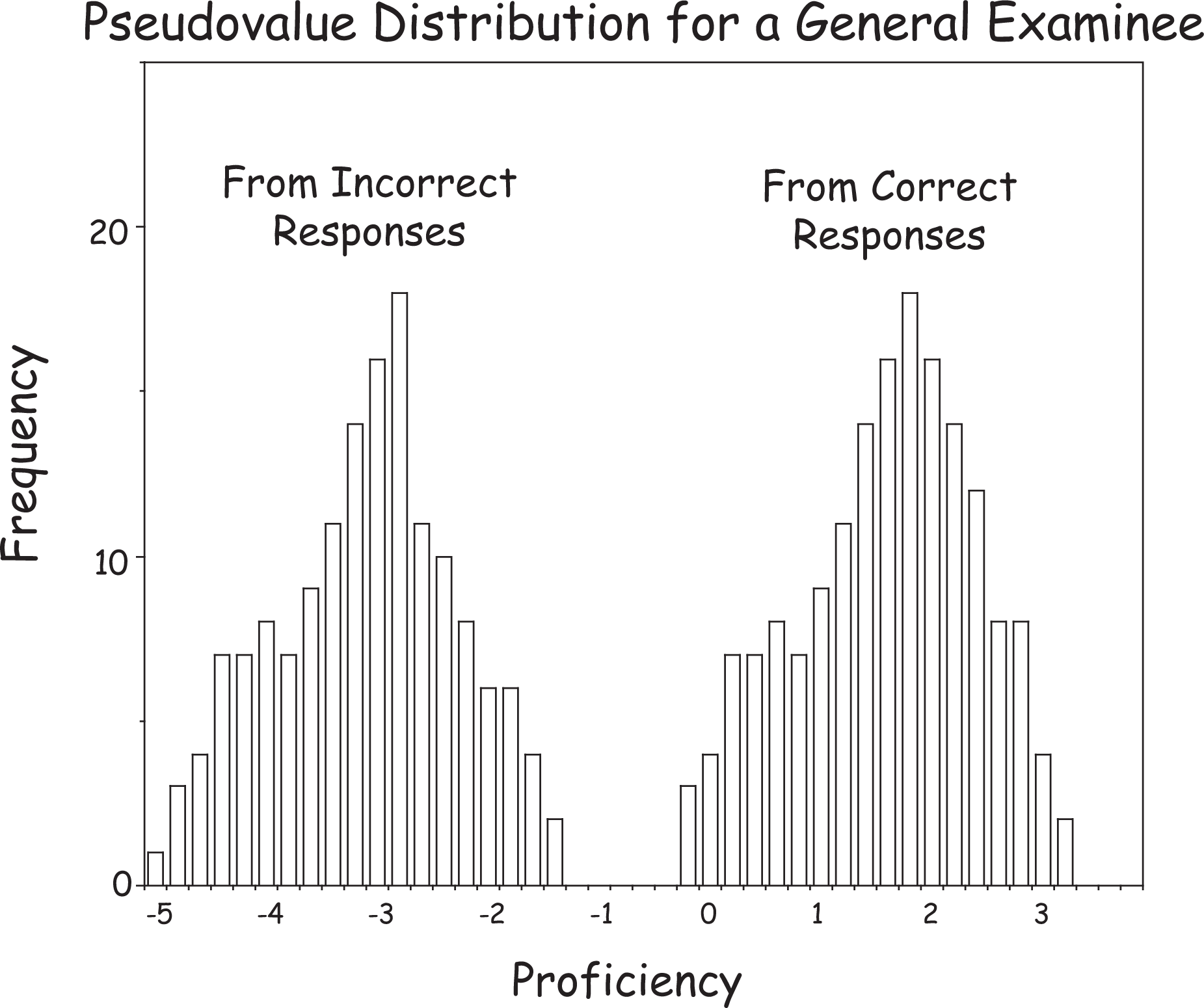
A typical pseudovalue distribution for a non-Optima examinee.

Let us imagine what the right-hand distribution would look like if an examinee had access to a subset of the test items in advance. In the extreme, we might expect to find a bimodal distribution of pseudovalues in which the central core of items represents the examinee’s true proficiency and the upper distribution is epiphenomenal, showing the effect of having access to some hard items in advance. Of course, any easy items that were seen in advance would be undetectable. One illustrative result is shown in Figure 2. Note the bimodal structure of the rightmost distribution. Our experience has taught us that such a result is akin to Thoreau’s “trout in the milk.”²

Figure 2.

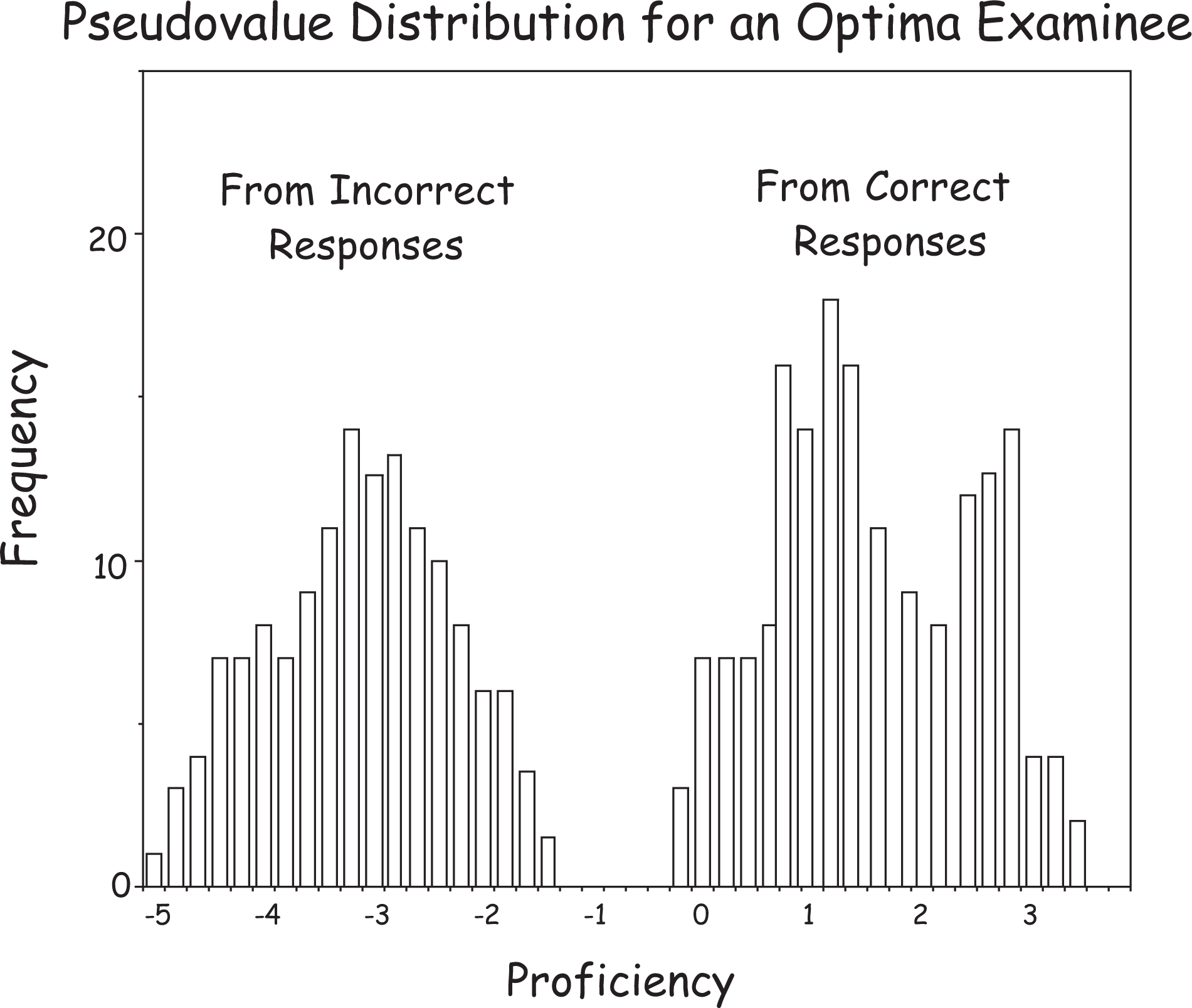
An illustrative pseudovalue distribution for an Optima student.

In the usual jackknife, we would merely use the mean of all the pseudovalues in each distribution and then use a weighted combination of them to yield the estimate of proficiency. But this is not the usual circumstance. Instead, we will view the distribution of pseudovalues as a contaminated distribution, and we want to obtain an estimate that down weights the contaminants. To accomplish this, we used a specific redescending M-estimator (Andrews et al., 1972) that was suggested by John Tukey (the biweight) and subsequently used to increase the robustness of IRT proficiency estimation by Mislevy and Bock (1982). This yields a robust estimate of θ that heavily weights the estimates in the main body of the distribution and down weights extreme values considerably. Indeed, if data values get extreme enough, they are not counted at all.

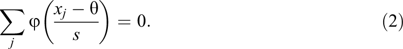
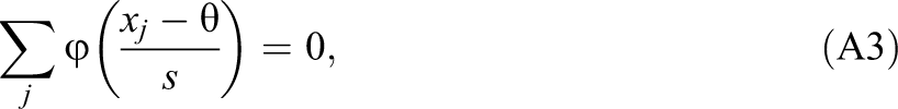
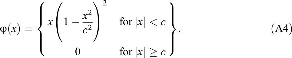
The proficiency parameter, θ, is estimated from Equation 2, where $ϕ (x)$ is the influence function (shown in Equation 3), x_j , is the binary item-level response where x_j = 1 if item j is answered correctly and zero otherwise, and s is some measure of spread; we use the median absolute deviation (MAD), a common robust choice, other options are possible:

\sum_{j} ϕ (\frac{x_{j} - θ}{s}) = 0.

Tukey’s biweight estimator has an influence function shown in Equation 3 and depicted graphically in Figure 3. Tukey’s biweight function has a tuning parameter c that simultaneously controls when the function turns back toward zero as well as determining the point after which an observation has no influence. Our explorations confirm Tukey’s suggestion that 4.7 is a good general value:

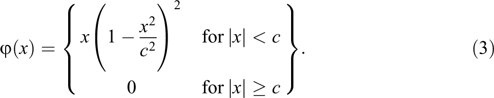
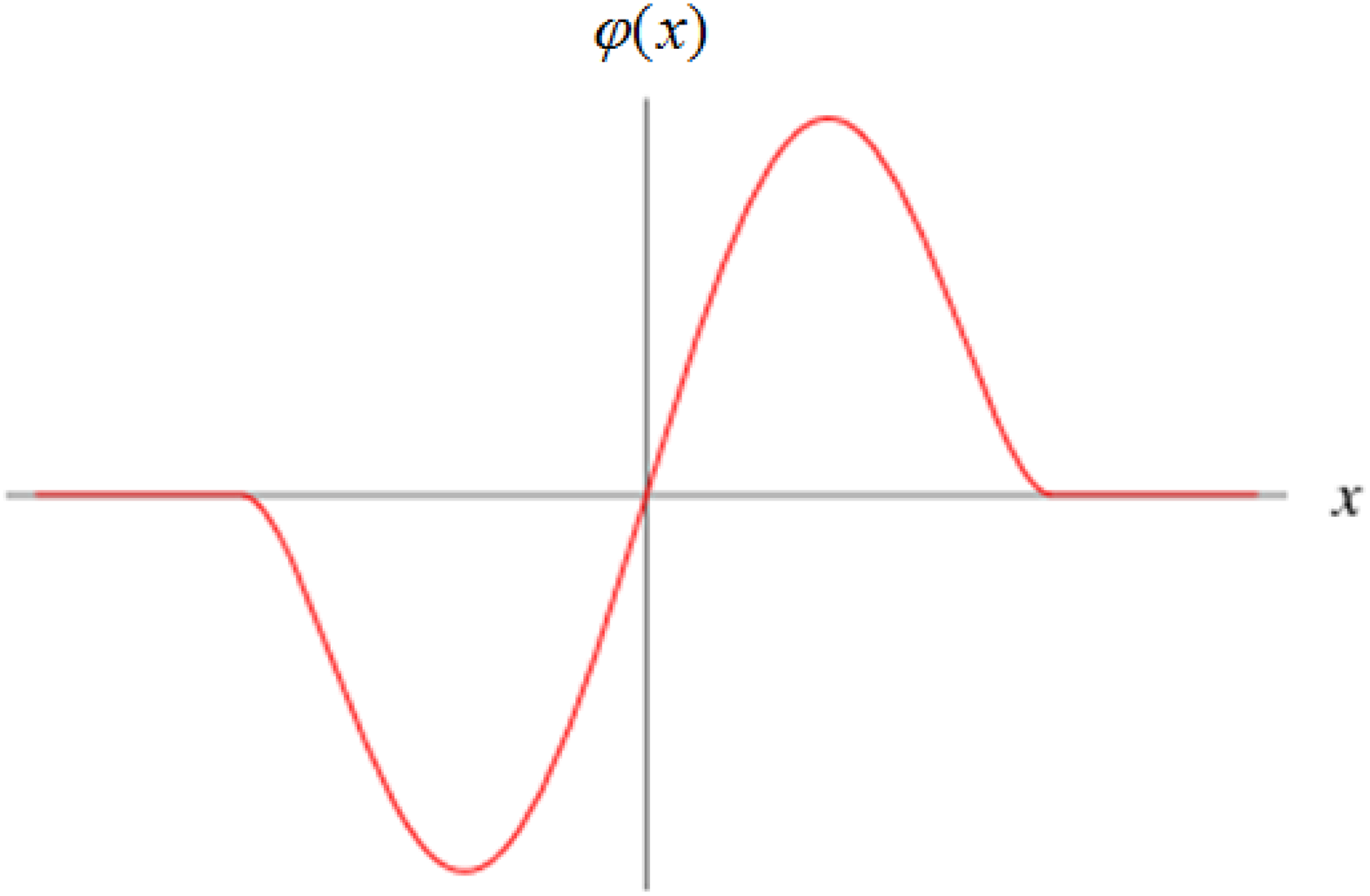
ϕ (x) = \{\begin{matrix} x {(1 - \frac{x^{2}}{c^{2}})}^{2} & for | x | < c \\ 0 & for | x | \geq c \end{matrix}\} .

Figure 3.

Influence function for Tukey’s biweight.

Testing the Method

We limited our study to only items that were used in our 2006 data set on the first part (Step 1) of the USMLE. We worked with a 2006 Step 1 data sample including 41,211 test takers. Of that number, we used a sample of 111 of them (0.27%) for whom there was evidence of Optima attendance. While this number does not purport to include all Optima attendees or others with prior exposure to examination content, we assume that such individuals represent a very small proportion of the total cohort of examinees. If our assumption is correct, it raises what may be the most difficult problem in detecting prior exposure—false positives. We shall discuss this issue in greater depth at the conclusion of this article.

Examinees were randomly assigned to one of dozens of forms of USMLE Step 1. Only a proper subset of 350 items on each form were scored; the rest are anchor or pretest items. The percentage of stolen items and numbers of Optima students for each form varied widely.

For purposes of our sample, the majority of items on all forms were not exposed, and for the vast majority of the forms, only a small percentage of the items were exposed. What this means operationally is that our procedure, relying, as it does, on the majority of the items yielding an unbiased estimate of the examinee’s proficiency will be appropriate.

As we might expect, a substantial proportion (45%) of Optima students had previously failed Step 1 (why else would they be taking an expensive coaching course), whereas only 17% of the other examinees were retaking the exam.

As a preliminary investigation of the size of the bias generated by the exposure of some of the items, we calculated the traditional maximum likelihood estimate (MLE) of each examinee’s score and also the MLE of his or her score using only those items that we knew had not been exposed. We found that the difference between these two figures was predictably larger, the more items that were exposed in that examinee’s form. The results of this analysis are shown in Figure 4.

Figure 4.

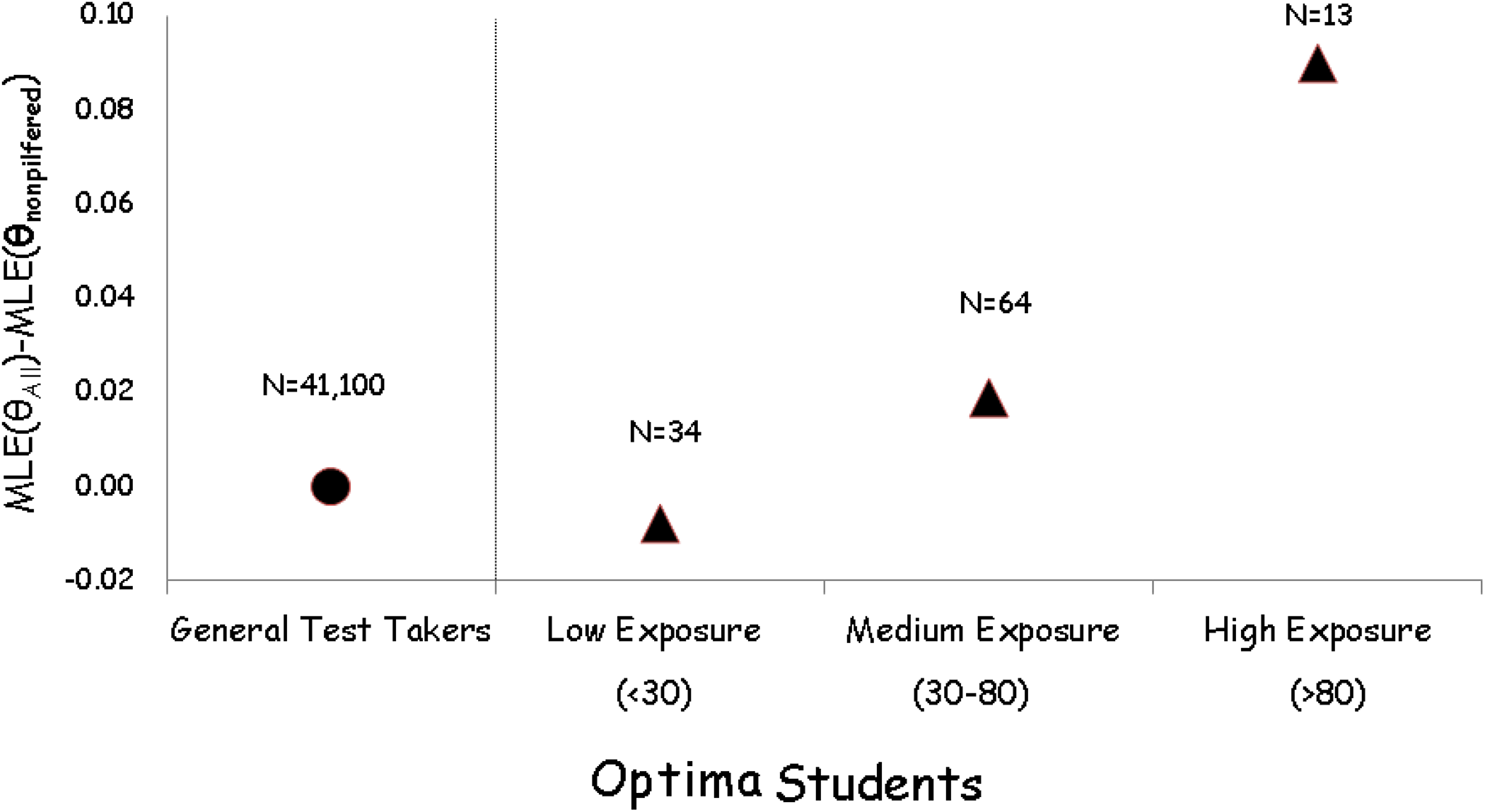
The more the items that were exposed prior to the test administration, the greater the difference between the estimates of the score based on all the items and the estimates based on just the secure items.

We then examined the extent to which this bias is reduced by applying our robust estimator of proficiency within each of the component score distributions of pseudovalues. The distributions of pseudovalues for Optima students are more widely dispersed than for general examinees (average MAD of 3.4 vs. 2.1, respectively). Moreover, the distributions of pseudovalues for Optima students tend to be either bimodal (as shown in Figure 2) or very platykurtic.³ We found that the robustification had only a small effect on the general test takers but a much larger effect on the Optima students. These results are summarized in Figure 5. Bias is defined as the difference between proficiency estimates from all items (estimated by either MLE or the biweight method) and the MLE of proficiency estimated from only nonpilfered items.

Figure 5.

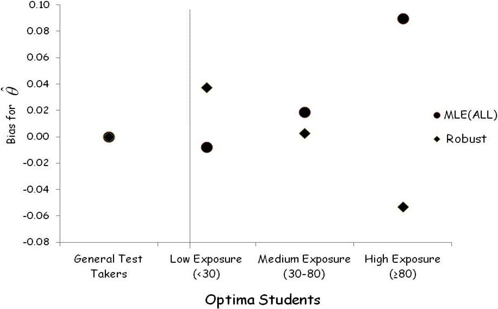
Comparing the bias in test scores for the traditional score estimate with the robust estimator.

The average bias for robust proficiency estimates of Optima students with medium exposure to pilfered items is essentially zero. But for Optima students with high exposure, what seems to be a negative bias appears. Why? We cannot be sure but two explanations seem plausible. First, maximum likelihood estimates for all items, pilfered and nonpilfered, are likely elevated due to successful guessing (remember that this test is scored with the 1-PL, and so it makes no correction for guessing).⁴ This explanation would explain why we would see a greater effect on Optima students than on the others, for the Optima students have, on average, lower proficiency and hence greater opportunity to guess. But it does not explain why the various Optima groups would be affected differentially. We would expect that the largest effects would be for the smallest groups because the standard error goes as the square root of n. Thus, we would anticipate that the variability for a group of 13 examinees would be more than twice that of a group of 64. We suspect that this is why we observed that Optima students with low exposure to pilfered items had a small positive bias.

On average, the robust proficiency estimates have almost no effect on general test takers. Some general test takers have a slightly higher proficiency estimate, perhaps due to the correction for carelessness; some of them have slightly lower proficiency estimate due to the correction for guessing.

We were concerned that some or all of the effect we observed might have been due to a shrinkage effect due to the Optima students being so far below the level of the other examinees. To assess the extent of such confounding, we matched 13 Optima students with high exposure with the almost 5,000 general test takers who had approximately the same scores, determined from only nonpilfered items. We found that even after matching, the robust estimators still worked well. Our results are shown in Figure 6. We postulate that the small positive bias for general test takers after matching may have resulted from the small correction for carelessness that this estimation method provides.

Figure 6.

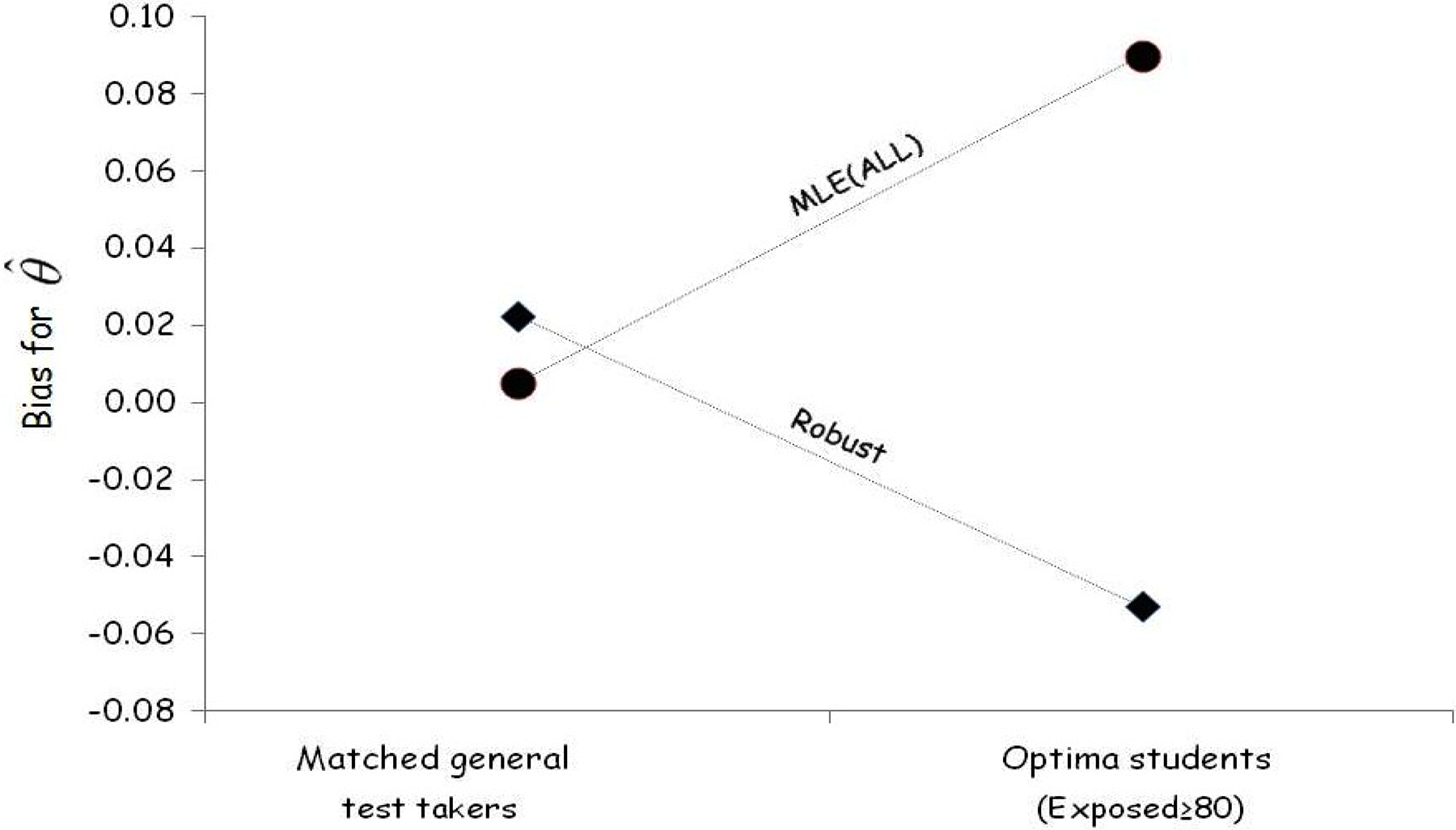
Comparing the bias in test scores for the traditional score estimate with the robust estimator. The comparison is being done for a matched sample (matched on total score) of general test takers and Optima students.

To provide insight into the size and the direction of the effect of our estimation method, it is useful to examine its results in the context of the variability of an individual’s response pattern. In Figure 7, we show the two distributions of pseudovalues for 1 of the 13 Optima students who was exposed to the items that eventually found their way onto the form that was administered. The various pseudovalues span a huge range of more than 10 logits. The estimate of proficiency that is generated from just the nonpilfered items is −1.32, whereas the unfiltered estimate from all items was higher, at −1.16. The robust estimator moves a little more than half way between these two values, to −1.25.

Figure 7.

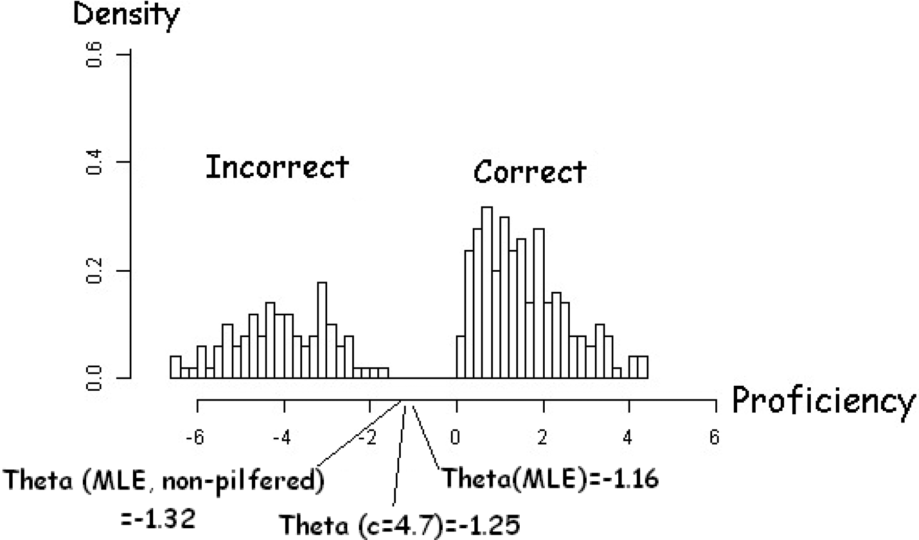
Pseudovalue distributions for an Optima student with high exposure (pilfered items > 80).

Note that this correction is amoral. It does not care whether the aberrant responses were due to advance information, specialized knowledge, or lucky guesses. It merely recognizes that the proficiency estimates generated by these responses are sufficiently far away from the general picture to cast doubt on their validity and so reduces their influence on the final estimate. The result of this is an estimate that has increased validity and reduced variability.

Conclusions and Discussions

A test score loses its validity, hence its value, if an examinee answers an item correctly for reasons unrelated to those talents being tested. Hence, we must worry about prior exposure to test content because it is a threat to the score’s validity. Only under very rare circumstances is the test administrator interested in the probity of the examinee for its own sake.⁵ Thus, the goal of considering the effects of prior access to content is to affirm the score’s validity not the probity of the examinee.

Reasons supporting this conclusion range from moral to practical. We will leave the discussion of the moral issues to other accounts (e.g., Hubert & Wainer, 2012) and focus instead on the practical ones, specifically on how difficult it is to identify cheaters to an acceptable level of accuracy. The reason this is so hard is because of the confluence of limited statistical evidence and the rarity of cheaters. Let us illustrate this explicitly.

Suppose we have a statistical method for identifying cheaters that, for the sake of argument, is 90% accurate. What we mean by this is that if a person is a cheater, 90% of the time we will identify them as such; and if a person is not a cheater, 90% of the time our statistical identification will testify to their innocence.

Stated in mathematical notation:

P (+ ID | Cheater) = .90,

P (- ID | Not Cheater) = .90.

But, these probabilities are not of direct interest because we do not know, a priori, whether or not someone is a cheater; all we know is what our statistical evidence says.

What we want to know is

P (Cheating| +ID),

P (Not cheating| - ID) .

Obviously, we need to use Bayes’s rule to reverse the direction of the conditional probabilities in Equations 4a and 4b. Let us do this for the situation we are faced with in the Optima case. We can calculate the probability in Equation 5a directly.

This probability is a fraction in which the numerator is the number of cheaters correctly identified, and the denominator is the number in the numerator plus the number of false positives (noncheaters identified as being cheaters). The numerator first: Using our sample of 111 examinees enrolled in Optima who had access to test questions in advance, 90% of these means that we will find 99 individuals. Next the denominator: This has the true positives identified, 99, plus 10% of the approximately 41,100 noncheaters who are identified incorrectly or 4,110. Thus, the denominator of this fraction is 99 + 4,110 or approximately 4,200.

Thus, the probability of someone actually being a cheater, given they were so identified, is 99/4,200 or approximately 1/42. Thus, for every person correctly identified as being a cheater, there would be 41 innocent people also accused.

This illustrates vividly the problem of false positives that we mentioned earlier in this article. Of course, most statistical methods for the identification of cheaters are nowhere close to 90% accurate, so this estimate is likely wildly optimistic. But, even if it were this accurate so long as the number of noncheaters vastly outnumbers the number of cheaters, this same effect will manifest itself. It may be worthwhile to absorb the high cost of false positives if the losses associated with allowing a cheater to get through are, in this case, 42 times higher than the losses associated with accusing an innocent examinee.

But this enormous uncertainty emphasizes the importance of modesty in the claims made for the discovery procedures. This is why wise testing organizations do not accuse any examinee of malfeasance because of fallible statistical evidence and have eschewed any sort of draconian punishment. Instead, the typical outcome is to embargo the score and allow the examinee to retest. Such a consequence is surely an inconvenience for the examinee but in the end does not darken the examinee’s reputation nor stifle their career plans.

The methodology we developed in this study matches this modest philosophical viewpoint. We purify the estimate of the examinee’s score by down weighting the contribution to that score of all unlikely responses. This can be to the examinee’s benefit by reducing the impact of very easy items that were inappropriately missed or, in the situation that got our attention in the first place, by reducing the score gain due to correct responses to items much more difficult than the examinee is able. This means that the examinee would not get any advantage of getting hard items right because they had prior exposure or because they guessed the answer correctly. We suspect that the small change in the scores of the general test takers after robust estimation is likely due to some of those examinees, for whatever reason, answering some items correctly that were more difficult than they were able.

This result makes explicit the key property of this methodology: We do not need to know in advance which items were exposed to be able to correct for the bias introduced by their exposure. Indeed, if we had such advance knowledge, this procedure is unnecessary. The data set developed in connection with the investigation and litigation concerning Optima allowed us to test this method when we already knew at least part of the answer.

Thus, the robust jackknife increases the validity of the scores as well as the efficiency of its estimators. It does both of these by simultaneously reducing bias and variance. This seems a pretty good deal for a very small expenditure in calculation.

Limitations and Discussions

We cannot end without a brief recapitulation of three of the limitations of our method as well as a discussion of four other questions that reviewers/editors raised.

Limitations

First, it is designed to work when only a minority of the items in a test form have been exposed. If the majority of items were exposed, the estimation method would add to the bias.

Second, we applied our method to low-proficiency test takers who had advanced information on test items, and we found that robust proficiency estimates work well to reduce bias in proficiency estimate. It is not likely to work well with high-proficiency test takers since the contaminated aspects of the response vector may not be aberrant enough to detect.

Third, essential unidimensionality⁶ may, to some extent, be a necessary condition, since we down weight misfitting items. We don’t know how quickly our method’s efficacy deteriorates as the test deviates from unidimensionality. We suspect that if there is a truly multidimensional test, it makes more sense to utilize our method on each unidimensional subscore separately.

Discussion and Additional Emphases

How is our method likely to work with small samples? Remember that all of the wonderful properties that we know and love of maximum likelihood estimators are asymptotic; its small sample shortcomings are well known (especially in sensitivity studies, Lewis, 1970). A pleasant surprise that emerged from the simulations we used to test our method 40 years ago was how much better it performed over MLEs in small samples. The smaller the sample, the greater the advantage it conferred. These advantages were in both validity (smaller bias) and efficiency (it was superefficient relative to MLEs).

Does this method yield issues in high-stakes testing for candidates with marginally passing scores? It is true that the reversal of ordinary shrinkage that this robustification manifests may cause some scores that were marginally passing to slip below the cut-score. Whether this is important depends on the loss function. The test we were concerned about, the USMLE, is certainly high stakes; if you pass, you get to practice medicine; if you fail, you cannot. Of course, if you fail, you can take it again. Unfortunately, those who pass through a quirk of chance, get admitted to practice even though if they were to take it again they would likely not pass. The loss function usually attested to by NBME is that it is far worse for an incompetent person to pass than for a marginally competent one to fail. Thus, concerns about an occasional false negative due to stochastic shrinkage must be weighed against the far greater good of keeping incompetent candidates out of medicine.

Why the 1-PL and not a weaker model (e.g., 2-PL or 3-PL)? As stated earlier, we used the 1-PL because that is the scoring model used by NBME to score the USMLE. Our outcomes would have been of lesser relevance to our employer had we opted for a weaker (more general) model. The upside of our choice is that it leaves open the further exploration of this methodology for a worthy graduate student in search of thesis topic.

Wouldn’t a series of simulations be revealing of exactly how this methodology works? Indeed, they have been (see the simulations we did 40 years ago—Wainer & Wright, 1980), and I have no doubt doing more of them would shed additional light. But useful scientific explorations are endless, in stark contrast with the work-life of scientists (or at least this scientist). So this account ends here. And those same graduate students on the lookout for worthwhile thesis topics referred to previously could make a real contribution continuing the exploration of the efficacy of this method through simulations that we began four decades ago.

Technical Appendix

Data were fitted separately for each test administration with a 1-PL model using marginal maximum likelihood estimation in the LTM package in R (Rizopoulos, 2006). The test was a random group design in which were assembled parallel test forms that were randomly assigned to examinees. The effectiveness of this test administration method was confirmed since means and standard deviations for reported scores as well as other covariates (e.g., numbers of previous attempts to take USMLE) were essentially identical across all forms. Therefore, subsequent equating to assure that the IRT parameters were comparable across forms was deemed unnecessary. In general, items were easy relative to the ability distribution of the examinees, since the proportions of answering item right (P+) were very high. We then applied our scoring method, using jackknifed pseudovalues paired with a robust M-estimator (Wainer & Wright, 1980). Specifically, we did the following steps:

Step 1: Pure 1-Parameter Logistic Maximum Likelihood Estimation

We estimated ability for full scale by solving Equation 6 using the Newton–Raphson algorithm. We used the 1-PL (Equation A1); because item parameters were estimated from large samples, we introduced no serious error by treating them as known. We then solved for θ for total scores from one to L − 1. This shortcut is acceptable for the 1-PL because in this model, raw score is a sufficient statistic for θ. This yields a column vector with a length of L − 1.

\begin{array}{l} r_{} - \sum_{j} [\frac{exp (a * (θ_{} - b_{j})}{1 + exp (a * (θ - b_{j})}] = 0, \\ r_{} = total score, \\ a_{} = common item discrimination parameter, \\ b_{j} = item difficulty parameter, \\ θ = theta estimates. \end{array}

Step 2: Jackknife Pseudovalues

To calculate the jackknife pseudovalues, we construct a matrix of abilities, W. If there are L items, matrix W has L rows and L + 1 columns. The first column of W matrix is estimated ability on the entire test derived from the first step for all possible raw scores. The remaining columns are derived by sequentially omitting each item in turn and then recalculating ability.

Each examinee has response vector of length L with elements x_j , where x_j = 1 if item j is answered correctly and zero otherwise. Therefore, we have (L − 1)*L ability estimates. These ability estimates are elements in ability matrix W or the ability estimates for test takers with varying total score levels from one to L − 1 and leaving out one jth item.

Each pseudovalue, $θ_{j}^{*}$ , can be easily calculated for each item using matrix W and Equation A2. We emphasize that the pseudovalues are the components of the influence function derived by leaving out 1 item and using them we can instantly see the extent to which the ability estimate is affected by a single item. Obviously, we are concerned when a small group of items exerts an undue amount of influence:

θ_{j}^{*} = n θ_{All} - (n - 1) θ_{(j)} .

The traditional jackknife estimate, $θ^{*}$ , is just the average of all pseudovalues, which can by itself reduce some potential bias. We have found that jackknife estimate is a little bit lower than maximum likelihood estimates. However, we are concerned here with an unusual circumstance, in which there are many aberrant response patterns requiring greater protection. It thus makes sense to use a more robust method than simply the arithmetic mean to the pseudovalue vectors.

Step 3: Robust M-estimator: Tukey’s Biweight

We then applied Tukey’s biweight estimator as shown in Equations A3 and A4. We fit a robust regression and specify only the intercept in the model using MM-estimation algorithm (Yohai, Stahel, & Zamar, 1991) in the R package MASS. The Tukey’s biweight estimators thus became our ability estimates:

\sum_{j} ϕ (\frac{x_{j} - θ}{s}) = 0,

ϕ (x) = \{\begin{matrix} x {(1 - \frac{x^{2}}{c^{2}})}^{2} & for | x | < c \\ 0 & for | x | \geq c \end{matrix}\} .

We needed to optimize the tuning parameter, c, for Tukey’s biweight influence function. The criteria are (a) it has minimal effect on general test takers such that average bias equal to zero and variance of bias is minimal and (b) it reduces positive bias as much as we can for Optima students with exposure to pilfered items. Following these criteria, the optimal c for this particular data set was 5.3. This estimate almost surely capitalizes on chance and would thus not likely remain optimal on cross-validation. However, we have found that the gain from using such a locally optimal tuning parameter provides little substantive improvement over c = 4.7, the generally accepted value of the tuning parameter value that was recommended by Tukey. Thus, in the usual circumstances, when we know nothing about the extent or seriousness of the contamination, it is likely safe (in this, as in most things scientific) to follow Tukey’s advice.

Step 4: Scaling

Last, but not least, applying Tukey’s biweight estimator will likely change the score scales mean and variance. Therefore, we need to restandardize it such that ability estimates once again have a mean of zero and variance of one. Other scaling methods may also be applicable to place the obtained scores on the scale that is usually reported.

Footnotes

Authors’ Note

This work is collaborative in all respects and the order of authorship is alphabetical. The research was done while the first author was a summer intern at the National Board of Medical Examiners where the second author was then Distinguished Research Scientist.

Acknowledgments

We would like to express our gratitude to Peter Baldwin and Brian Clauser for their help at various stages of the project, especially in providing us with access to the data we use to test our method, and to Gerry Dillon, Shelley Green, and Ron Nungester for their advice about the USMLE and Optima and for helping us to more nearly say what we meant.

Declaration of Conflicting Interests

The author(s) declared no potential conflicts of interest with respect to the research, authorship, and/or publication of this article.

Funding

The author(s) received no financial support for the research, authorship, and/or publication of this article.

Notes

References

Andrews

D. F.

Bickel

P. J.

Hampel

F. R.

Huber

P. J.

Rogers

W. H.

Tukey

J. W.

(1972). Robust estimates of location. Princeton, NJ: Princeton University Press.

Hampel

F. R.

Ronchetti

E. M.

Rousseeuw

P. J.

Stahel

W. A.

(1986). Robust statistics: The approach based on influence functions. New York, NY: Wiley Interscience.

Hubert

Wainer

(2012). A statistical guide for the ethically perplexed. New York, NY: Chapman & Hall.

Lewis

(1970). The count-back method. Princeton, NJ: Educational Testing Service.

Mislevy

R. J.

Bock

R. D.

(1982). Biweight estimates of latent ability. Educational and Psychological Measurement, 42, 725–737.

Mosteller

Tukey

J. W.

(1968). Data analysis: Including statistics. In Lindsey

Aronson

(Eds.), The handbook of social psychology (pp. 80–203). Reading, MA: Addison-Wesley.

Quenouille

M. H.

(1956). Notes on bias in estimation. Biometrika, 43, 353–360.

Rizopoulos

(2006). LTM: An R package for latent variable modeling and item response theory analyses. Journal of Statistical Software, 17, 1–25.

Stout

W. R.

(1990). A new item response theory modeling approach with applications to unidimensionality assessment and ability estimation. Psychometrika, 55, 293–325.

10.

Thoreau

H. D.

(1968). The writings of Henry David Thoreau: Journal, vol. 2, 1850-September 15, 1851 . Torrey

Bradford

(Ed.), New York: AMS Press. From the edition of 1906.

11.

Tukey

J. W.

(1958). Bias and confidence in not-quite large samples (abstract). The Annals of Mathematical Statistics, 29, 614.

12.

Wainer

Bradlow

E. T.

Wang

(2007). Testlet response theory and its applications. New York, NY: Cambridge University Press.

13.

Wainer

Wright

B. D.

(1980). Robust estimation of ability in the Rasch model. Psychometrika, 45, 373–391.

14.

Yohai

V. J.

Stahel

W. A.

Zamar

R. H.

(1991). A procedure for robust estimation and inference in linear regression. In Stahel

W. A.

Weisberg

S. W.

(Eds.), Directions in robust statistics and diagnostics, Part II (pp. 365–374). New York, NY: Springer-Verlag.