Testing Latent Variable Distribution Fit in IRT Using Posterior Residuals

Abstract

This research proposes a new statistic for testing latent variable distribution fit for unidimensional item response theory (IRT) models. If the typical assumption of normality is violated, then item parameter estimates will be biased, and dependent quantities such as IRT score estimates will be adversely affected. The proposed statistic compares the specified latent variable distribution to the sample average of latent variable posterior distributions commonly used in IRT scoring. Formally, the statistic is an instantiation of a generalized residual and is thus asymptotically distributed as standard normal. Also, the statistic naturally complements residual-based item-fit statistics, as both are conditional on the latent trait, and can be presented with graphical plots. In addition, a corresponding unconditional statistic, which controls for multiple comparisons, is proposed. The statistics are evaluated using a simulation study, and empirical analyses are provided.

Keywords

item response theory model misspecification latent variable distribution

In item response theory (IRT), it is usually assumed that the probability distribution of the latent variable, say $g (θ)$ , is normal. However, researchers have argued that in some situations, the normality of $g (θ)$ may be a dubious assumption (Li & Cai, 2018; Reise et al., 2018; Woods, 2006; Woods & Thissen, 2006). For example, if multiple subpopulations are grouped together, then the combined $g (θ)$ may be multimodal or otherwise nonnormal (Li & Cai, 2018). Moreover, if this assumption is violated, then the IRT model is misspecified, and item parameter estimates will be biased. Additionally, this bias will impact subsequent estimates such as scale scores. Researchers and practitioners concerned with nonnormal $g (θ)$ can use more flexible IRT models (Bock & Aitkin, 1981; Mislevy, 1984; Woods & Lin, 2009; Woods & Thissen, 2006), but fitting such models requires additional model specification decisions (e.g., the number of quadrature points for an empirical histogram) and introduces parameters that may be challenging to interpret (e.g., Ramsay-curve spline coefficients). A potentially more convenient approach is to assume $g (θ)$ is normal during calibration and then evaluate the fit of $g (θ)$ (Béguin & Glas, 2001; Ferrando & Lorenzo-Seva, 2001; Li & Cai, 2018; Sinharay et al., 2006). If the normal distribution provides adequate fit, then a more flexible, and complex, model is arguably unnecessary.

In the current research, we propose a new statistic for testing latent variable distribution fit for unidimensional IRT models within a likelihood-based framework. A distinguishing feature of the proposed statistic is that it focuses on posterior distributions of latent variables commonly used in expected a posteriori (EAP) and maximum a posteriori (MAP) scoring procedures (Bock & Aitkin, 1981). More specifically, the statistic compares the sample average of posterior distributions to the specified (or estimated) $g (θ)$ . Extant methods for testing the fit of $g (θ)$ , on the other hand, focus on the comparison of sample and model-implied distributions of summed scores. These methods have proven useful in both likelihood (Ferrando & Lorenzo-Seva, 2001; Li & Cai, 2018) and Bayesian frameworks (Béguin & Glas, 2001; Sinharay et al., 2006). However, some information in the data is lost when response patterns are summarized by sum scores, and using the full response patterns, via posterior distributions, may prove advantageous when evaluating the fit of $g (θ)$ .

A second distinguishing feature of the proposed statistic is that it conditions on a fixed latent variable value just like some item-fit statistics (du Toit, 2003; Haberman et al., 2013; Hambleton & Swaminathan, 1985). An advantage of this feature is that the statistic lends itself to graphical plots, which have proven useful in evaluating item fit (Haberman et al., 2013; Muraki & Bock, 2003; van Rijn et al., 2016; Wells & Hambleton, 2016). As such, the proposed statistic may be considered a complement to such residual-based item-fit statistics. A drawback of this feature is that the proposed conditional statistic does not directly provide an overall test of the fit of $g (θ)$ across the range of $θ$ . With that said, the conditional statistics can be used to make an overall decision by adjusting for multiple comparisons. This unconditional statistic is also studied in the current research.

A third distinguishing feature of the proposed (conditional) statistic is that it is formally an instantiation of a generalized residual as proposed by Haberman and Sinharay (2013). The generalized residuals framework can be used to compare numerous sample quantities to model-implied counterparts, including proportion correct for a single item, proportion simultaneously correct for a pair of items, and summed score distributions (van Rijn et al., 2016). The current research shows that the framework is even more versatile and may also be used to evaluate the fit of $g (θ)$ . A major benefit of the framework is that generalized residuals are asymptotically distributed as standard normal, and therefore there is no need to develop asymptotic arguments for the proposed statistic. A secondary benefit is that generalized residuals may be applied, after incorporating weights, to large-scale educational survey assessments such as the National Assessment of Educational Progress (NAEP; van Rijn et al., 2016).

Methodological Background

This section first presents an example IRT model and some maximum likelihood (ML) theory. Second, Li and Cai’s (2018) summed score chi-square ( ${\bar{X}}^{2}$ ), used in the simulation study, is presented. Third, this section presents an overview of the generalized residuals framework of Haberman and Sinharay (2013). Finally, the proposed statistic to evaluate the fit of $g (θ)$ is presented as an instantiation of this framework.

Example IRT Model and ML Estimation

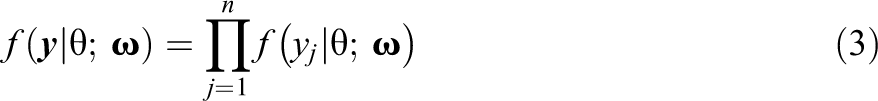
Let $Y = (Y_{1}, . . ., Y_{j}, . . ., Y_{n})'$ be a random vector with realization $y = (y_{1}, . . ., y_{j}, . . ., y_{n})'$ , where $y_{j} \in \{0, 1\}$ , and let $ω$ be a q-dimensional vector of all freely estimated parameters for the model. For the three-parameter logistic (3PL; Birnbaum, 1968) model, the conditional probability of endorsing item j is

P (Y_{j} = 1 |θ; ω) = g_{j} + \frac{(1 - g_{j})}{1 + exp [- (a_{j} θ + c_{j})]},

where $θ$ is the latent variable and a_j, c_j, and g_j are the discrimination, intercept, and pseudo-guessing parameters for the jth item, respectively. Then, let

f (y_{j} | θ; ω) = P {(Y_{j} = 1 |θ; ω)}^{y_{j}} {[1 - P (Y_{j} = 1 |θ; ω)]}^{1 - y_{j}}

be the conditional probability that $Y_{j} = y_{j}$ . Under the assumption of conditional independence, let

f (y |θ; ω) = \prod_{j = 1}^{n} f (y_{j} |θ; ω)

be the conditional probability that $Y = y$ . Next, let $g (θ; ω)$ be the distribution of the latent variable, and let $f (y, θ; ω) = f (y |θ; ω) g (θ; ω)$ be the joint probability density. Often, $g (θ; ω)$ is assumed to be standard normal, in which case it does not depend on $ω$ . The marginal probability of an observed response pattern is

π (y; ω) = \int f (y, θ; ω) d θ .

Next, let there be N respondents, and let p_y be the observed proportion of respondents with response pattern y . Let $Y$ be the set of $C = 2^{n}$ possible response patterns. Once observed, the response patterns are treated as fixed, and the log-likelihood may be written as

L (ω) \propto \sum_{y \in Y}^{} p_{y} l (ω; y),

where $l (ω; y) = logπ (y; ω)$ . Maximization of the log-likelihood (e.g., Bock & Aitkin, 1981) yields the ML estimates of the item parameters, $\hat{ω}$ .

Suppose that $π_{0} (y)$ is a true (population) response pattern probability. Then, if the IRT model is correctly specified, there is a parameter vector $ω_{0}$ such that $π_{0} (y) = π (y; ω_{0})$ , $y \in Y$ . The asymptotic distribution of the MLE $\hat{ω}$ is normal,

\sqrt{N} (\hat{ω} - ω_{0}) \overset{d}{\to} N (0, F_{0}^{- 1}),

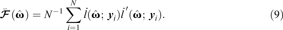
where $F_{0} = F (ω_{0})$ is the population Fisher information matrix for one observation. This matrix is defined as

F (ω) = \sum_{y \in Y}^{} π (y; ω) \dot{l} (ω; y) {\dot{l}}^{′} (ω; y),

where

\dot{l} (ω; y) = \frac{\partial logπ (y; ω)}{\partial ω},

is a q-dimensional vector of partial derivatives. Because $ω_{0}$ is unknown, $F_{0}$ must be estimated in practice, and one convenient estimator is the sample cross-product approximation (Meilijson, 1989)

\bar{F} (\hat{ω}) = N^{- 1} \sum_{i = 1}^{N} \dot{l} (\hat{ω}; y_{i}) {\dot{l}}^{′} (\hat{ω}; y_{i}) .

Evaluating Latent Variable Distribution Fit Using Sum Scores

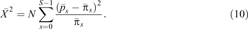
To the best of our knowledge, extant methods for evaluating latent variable distribution fit are based on summed scores (see Li & Cai, 2018, and the references therein). For n items, each with K categories, there are $S = 1 + n (K - 1)$ possible summed scores, ranging from 0 to $S - 1$ . Let ${\bar{p}}_{s}$ be the observed summed score proportions for $s = 0, . . ., S - 1$ . And, let ${\bar{π}}_{s}$ be the corresponding model-implied summed score probabilities, for $s = 0, . . ., S - 1$ . Then, a Pearson-type statistic may be written as

{\bar{X}}^{2} = N \sum_{s = 0}^{S - 1} \frac{{({\bar{p}}_{s} - {\bar{π}}_{s})}^{2}}{{\bar{π}}_{s}} .

This statistic has been used in both likelihood (Ferrando & Lorenzo-Seva, 2001; Li & Cai, 2018) and Bayesian (Béguin & Glas, 2001; Sinharay et al., 2006) frameworks to evaluate latent variable distribution fit or, more generally, overall model fit. Within a Bayesian framework, ${\bar{X}}^{2}$ may be used via posterior predictive model checking (e.g., Sinharay et al., 2006) to evaluate the fit of $g (θ)$ . Within a likelihood framework, Li and Cai (2018) proposed a reference distribution for ${\bar{X}}^{2}$ , under the null hypothesis that the latent variable distribution is correctly specified in the IRT model. Specifically, the authors demonstrated that under a broad range of practical settings, the tail-area probabilities of ${\bar{X}}^{2}$ can be well-approximated by a χ² distribution with $S - 1 - 2$ degrees of freedom.¹

Generalized Residuals for IRT

The purpose of this section is to present a summary of the Haberman and Sinharay (2013) generalized residuals framework to facilitate the presentation of the proposed statistic in the next section. Interested readers are referred to Haberman and Sinharay (2013) for greater detail (see also Haberman, 2009; Haberman et al., 2013).

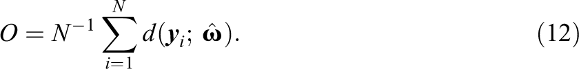
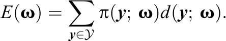
Let $d (y; ω)$ be a real continuous function on the parameter space $Ω$ , with corresponding ML estimate $d (y; \hat{ω})$ . The (model-implied) expectation of $d (y; ω)$ is

E (ω) = \sum_{y \in Y}^{} π (y; ω) d (y; ω),

with corresponding ML estimate $\hat{E} = E (\hat{ω})$ . Let O be the sample mean of the $d (y_{i}; \hat{ω})$ ,

O = N^{- 1} \sum_{i = 1}^{N} d (y_{i}; \hat{ω}) .

Then, the difference between the observed and expected values, $(O - \hat{E})$ , can serve as the basis for a test statistic given the availability of an estimate of the corresponding standard error. The asymptotic variance of $\sqrt{N} (O - \hat{E})$ is the minimum over the q-dimensional vector c of the expectation

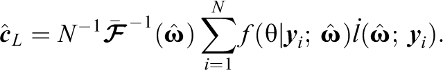
σ^{2} (ω_{0}) = \sum_{y \in Y}^{} π (y; ω_{0}) {[d (y; ω_{0}) - E (ω_{0}) - c^{'} \dot{l} (ω_{0}; y)]}^{2},

where the optimal value of c is

c (ω_{0}) = F^{- 1} (ω_{0}) \sum_{y \in Y}^{} π (y; ω_{0}) d (y; ω_{0}) \dot{l} (ω_{0}; y),

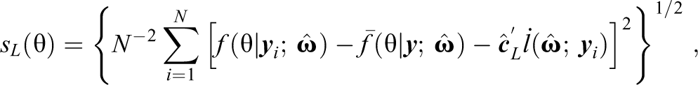
(Haberman & Sinharay, 2013, pp. 1442-1443). A consistent estimator of this asymptotic variance $σ^{2} (ω_{0})$ is the sample average

{\hat{σ}}_{L}^{2} = σ_{L}^{2} (\hat{ω}) = N^{- 1} \sum_{i = 1}^{N} {[d (y_{i}; \hat{ω}) - O - {\hat{c}}_{L}^{'} \dot{l} (\hat{ω}; y_{i})]}^{2},

with

{\hat{c}}_{L} = c_{L} (\hat{ω}) = N^{- 1} {\bar{F}}^{- 1} (\hat{ω}) \sum_{i = 1}^{N} d (y_{i}; \hat{ω}) \dot{l} (\hat{ω}; y_{i}),

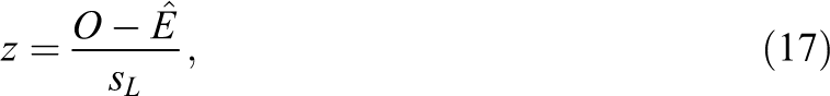
where $\bar{F} (\hat{ω})$ is computed as in Equation 9. Haberman and Sinharay (2013) refer to generalized residuals using the variance estimator in Equations 15 and 16 as Louis (1982) residuals, hence, the subscripts of L.² Let $s_{L} = {\hat{σ}}_{L} / \sqrt{N}$ be the corresponding standard error estimate for $(O - \hat{E})$ . Then, the generalized residual is

z = \frac{O - \hat{E}}{s_{L}},

which converges to a standard normal distribution under the null hypothesis that the model is correctly specified (Haberman & Sinharay, 2013).

Proposed Residual Based on Posterior Distributions

The proposed residual in this research depends on the posterior distribution of $θ$ , which, by Bayes’s theorem, is

f (θ| y; ω) = \frac{f (y |θ; ω) g (θ; ω)}{π (y; ω)} .

The expectation of $f (θ| y; ω)$ , over the distribution of the observed data y , is simply $g (θ; ω)$ . This is because a marginal distribution can always be expressed as an expectation, in this case:

g (θ; ω) = \sum_{y \in Y}^{} π (y; ω) f (θ| y; ω) .

Restating Equation 11 for convenience, the expected value of $d (y; ω)$ , needed for z, is

E (ω) = \sum_{y \in Y}^{} π (y; ω) d (y; ω) .

Comparing these expressions, it is apparent that a residual within the Haberman and Sinharay (2013) framework may be defined based on $d (y; ω) = d (y, θ; ω) = f (θ| y; ω)$ , with corresponding expectation $E (ω) = E (θ; ω) = g (θ; ω)$ . Then, for this choice of d, the proposed posterior residual is

z (θ) = \frac{O (θ) - \hat{E} (θ)}{s_{L} (θ)} = \frac{\bar{f} (θ| y; \hat{ω}) - g (θ; \hat{ω})}{s_{L} (θ)},

where $\bar{f} (θ| y; \hat{ω}) = N^{- 1} \sum_{i = 1}^{N} f (θ| y_{i}; \hat{ω})$ is the sample average of posterior distributions, $g (θ; \hat{ω})$ is the ML estimate of the distribution of the latent variable, and $s_{L} (θ)$ is the corresponding standard error estimate. For the proposed posterior residual, applying Equations 15 and 16 with $d (y, θ; ω) = f (θ| y; ω)$ ,

s_{L} (θ) = {\{N^{- 2} \sum_{i = 1}^{N} {[f (θ| y_{i}; \hat{ω}) - \bar{f} (θ| y; \hat{ω}) - {\hat{c}}_{L}^{'} \dot{l} (\hat{ω}; y_{i})]}^{2}\}}^{1 / 2},

with

{\hat{c}}_{L} = N^{- 1} {\bar{F}}^{- 1} (\hat{ω}) \sum_{i = 1}^{N} f (θ| y_{i}; \hat{ω}) \dot{l} (\hat{ω}; y_{i}) .

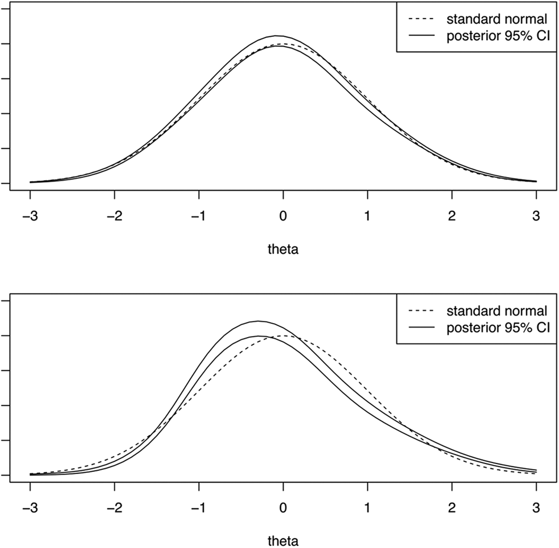
Thus, the proposed residual discrepancy compares $\bar{f} (θ| y; \hat{ω})$ and $g (θ; \hat{ω})$ , which both converge in probability to $g (θ; ω_{0})$ when the model is correctly specified. If $g (θ; ω)$ is assumed standard normal, then $z (θ)$ simply compares $\bar{f} (θ| y; \hat{ω})$ and a standard normal. Analogous to the item-fit plots in Haberman et al. (2013), latent variable distribution fit plots can be created by plotting $g (θ; \hat{ω})$ and the confidence band provided by $\bar{f} (θ| y; \hat{ω}) - 2 s_{L} (θ)$ and $\bar{f} (θ| y; \hat{ω}) + 2 s_{L} (θ)$ . Two example latent variable distribution fit plots are presented in Figure 1. In each plot, the dotted line denotes $g (θ; \hat{ω})$ , assumed standard normal in both examples. The solid lines represent pointwise 95% confidence bands, and dots outside the lines correspond to statistically significant residuals. In the top panel of Figure 1, the plot shows that $g (θ)$ fits well overall though there are some significant residuals around $θ = 1$ and $θ = 2$ . In contrast, in the bottom panel of Figure 1, the plot shows that $g (θ)$ appears to fit poorly across the range of $θ$ .

Figure 1.

Example of latent variable distribution fit plots. Note. CI $=$ confidence interval. Plots correspond to fitting two-parameter logistic models to International Cognitive Ability Resource (ICAR) data set (Condon & Revelle, 2014; top panel) and science assessment data from the TESTFACT (Wood et al., 2003) manual (bottom panel). Pointwise 95% CIs created by adding and subtracting two standard errors to the average of the individual posterior distributions.

Because the posterior $f (θ| y; ω)$ depends on both $g (θ; ω)$ and $f (y |θ; ω)$ , the statistic $z (θ)$ may be sensitive to misspecification of either the latent variable distribution or item models. In somewhat related work, Sinharay et al. (2006) demonstrated that summed score–based discrepancies can be effective for evaluating the fit of $g (θ; ω)$ as well as item fit at the test level (i.e., with one statistic). For these reasons, we conjecture that the proposed residual $z (θ)$ may also be sensitive to (overall) item misfit. This possibility is explored in the simulation study.

Adjusting for multiple comparisons

As previously mentioned, an advantage of the conditional nature of $z (θ)$ is that it characterizes the fit of $g (θ)$ across the range of $θ$ . However, practitioners might prefer to make an overall decision, that is, to test the null hypothesis that $g (θ)$ is correctly specified in the IRT model. As suggested by an anonymous reviewer, a straightforward way to adjust for multiple comparisons in the current setting is to use a Bonferroni correction. That is, for each quadrature node, $z (θ)$ can be tested using a Bonferroni-corrected significance level. Under this strategy, if the (conditional) null hypothesis is rejected for any of the statistics, then the overall null hypothesis is likewise rejected. This is equivalent to comparing the maximum absolute $z (θ)$ value, say z_B, to a Bonferroni-corrected critical value.

Note that unlike $z (θ)$ , z_B will not converge to a standard normal distribution. As with conditional item-fit statistics, the $z (θ)$ statistics are correlated across quadrature nodes (e.g., Haberman et al., 2013). Thus, at convergence, z_B can be expected to be somewhat conservative. Also note that the rate of convergence of z_B is determined by the slowest rate of convergence of $z (θ)$ across the quadrature nodes. Consequently, in some cases, very large samples may be needed for z_B to perform satisfactorily.

Simulation Study

Design

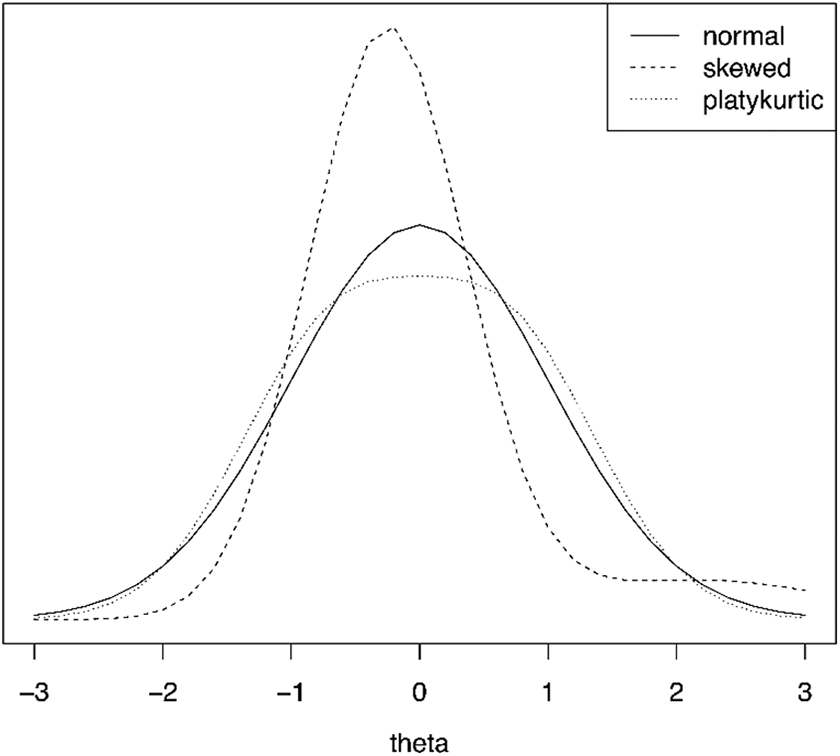
A simulation study was conducted to evaluate the performance of $z (θ)$ and z_B. The study included three test lengths (10, 20, and 40 items), three sample sizes (500, 1,000, and 2,000), and four data-generating latent variable distributions (normal, skewed, platykurtic, and bivariate normal). These levels were fully crossed. The skewed and platykurtic distributions were identical to those studied in Woods and Thissen (2006; see also Monroe & Cai, 2014; Sinharay et al., 2006) and are plotted in Figure 2. The correlation for the bivariate normal distribution was .9, identical to the distribution studied in Li and Cai (2018).

Figure 2.

Generating latent variable density functions for simulation study. Note. Skewed and platykurtic distributions were defined as normal mixtures based on generating parameters in Woods and Thissen (2006).

For each of these combinations of conditions, the true item model was a two-parameter logistic (2PL) model, which corresponds to Equation 1 with $g_{j} = 0$ . Discrimination parameters $a_{j}$ were drawn from a log-normal distribution ( $M = 0, S D = .2$ ). Difficulty parameters, b_j, were drawn from a normal distribution ( $M = 0, S D = .75$ ). Then, intercept parameters were calculated as $c_{j} = - a_{j} b_{j}$ . For the bivariate normal $g (θ)$ , one half of the items loaded on each dimension, creating between-item multidimensionality (Adams et al., 1997).

In addition, the test length and sample size levels were fully crossed along with a normal $g (θ)$ and a 3PL item model. Previous studies (Orlando & Thissen, 2000; Sinharay et al., 2006) have shown that detecting misfit when a 2PL model is fit to data generated under a 3PL model can be challenging. For the 3PL items, the pseudo-guessing parameters were drawn from a beta distribution ( $α = 8, β = 32$ ), and other item parameters were drawn as described above.

The calibration model was always a unidimensional IRT model with standard normal $g (θ)$ and 2PL model. In total, there were 45 sets of conditions: 9 under the null, 27 with a misspecified $g (θ)$ , and 9 with a misspecified item model. For each set of conditions, 500 replications were performed. All calibrations were performed using Bock and Aitkin’s (1981) expectation-maximization (EM) algorithm.

The impact of the various misspecifications was studied by evaluating the item parameter estimates and the item characteristic curve (ICC) estimates. To evaluate the item parameter estimates, the bias and root mean square error (RMSE) for the discrimination and difficulty parameters were collected. To evaluate the ICC estimates, a variant of the root mean square deviation item-fit statistic (Köhler et al., 2020) was used. In the current study, the variant of this statistic is defined, for the jth item, as

{RMSD}_{j} = {\{\int {[P_{j} (θ; \hat{ω}) - P_{j} (θ; ω_{0})]}^{2} g (θ) d θ\}}^{1 / 2},

where $P_{j} (θ; ω) = P (Y_{j} = 1 |θ; ω)$ is the ICC from Equation 1, and $g (θ)$ is the data-generating latent variable distribution. This ${RMSD}_{j}$ statistic provides a scalar-valued summary of the discrepancy between the estimated and true ICCs. In addition, the relative change ( $RC$ ) from the null condition ${RMSD}_{j}$ to each corresponding alternative condition ${RMSD}_{j}$ was computed.

To compute these statistics for the bivariate normal distribution, some complication arises because no true unidimensional ICC exists. To obtain a unidimensional ICC for comparison purposes, the data-generating two-dimensional model was reparameterized as a testlet response model (Thissen, 2013). Then, following Ip (2010), the testlet effect was integrated out to obtain a marginalized ICC. The resulting discrimination and difficulty parameters were treated as the true values.

For each replication, $z (θ)$ was computed for 31 evenly spaced grid points between $- 3$ and 3, a set of values previously used for studying conditional item-fit statistics (e.g., Haberman et al., 2013).³ The overall statistic z_B was also collected and tested using a Bonferroni-corrected significance level based on 31 comparisons. In addition, three other goodness-of-fit statistics were collected: ${\bar{X}}^{2}$ (Li & Cai, 2018) for evaluating the fit of $g (θ)$ , M₂ (Maydeu-Olivares & Joe, 2006) for evaluating overall model fit, and S − X² (Orlando & Thissen, 2000) for evaluating item fit. Calibrations and computation of ${\bar{X}}^{2}$ , M₂, and S − X² were performed using flexMIRT (Cai, 2017). The proposed statistics $z (θ)$ and z_B were computed using R (R Core Team, 2018).

Results for Estimation of Item Parameters and ICCs

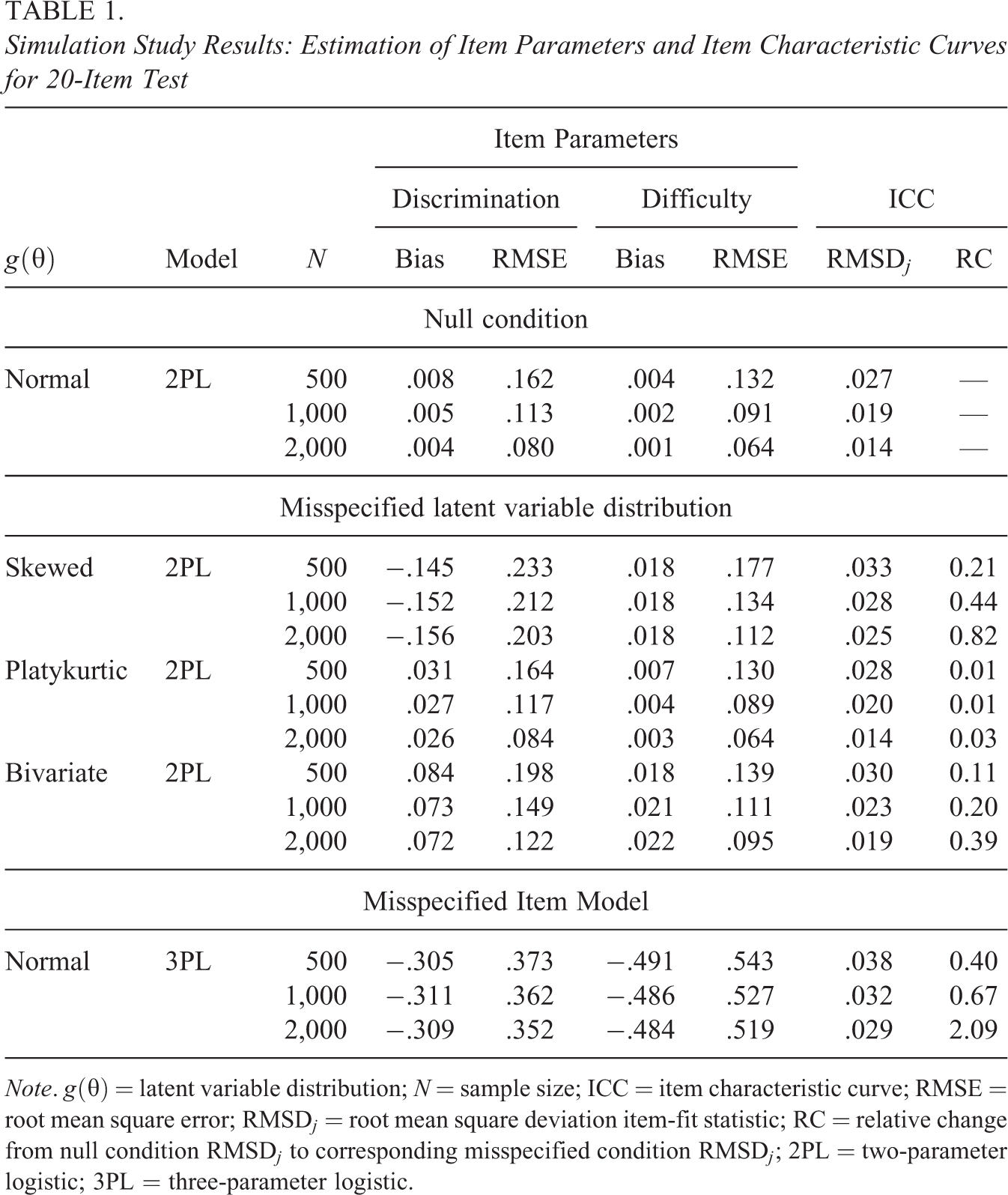
Table 1 presents results on the impact of the various misspecifications on the estimated item parameters and ICCs for the 20-item test length. The patterns of results for the other test lengths were similar and are not reported. The top section of the table gives results for the null condition and can be used as a baseline for interpreting the results for the alternative conditions. As expected, there is very little bias for the item parameter estimates, and both the RMSE and ${RMSD}_{j}$ statistics decrease as N increases.

Table 1.

Simulation Study Results: Estimation of Item Parameters and Item Characteristic Curves for 20-Item Test

$g (θ)$	Model	N	Item Parameters				ICC
			Discrimination		Difficulty		ICC
			Bias	RMSE	Bias	RMSE	${RMSD}_{j}$	$RC$
Null condition
Normal	2PL	500	.008	.162	.004	.132	.027	—
		1,000	.005	.113	.002	.091	.019	—
		2,000	.004	.080	.001	.064	.014	—
Misspecified latent variable distribution
Skewed	2PL	500	−.145	.233	.018	.177	.033	0.21
		1,000	−.152	.212	.018	.134	.028	0.44
		2,000	−.156	.203	.018	.112	.025	0.82
Platykurtic	2PL	500	.031	.164	.007	.130	.028	0.01
		1,000	.027	.117	.004	.089	.020	0.01
		2,000	.026	.084	.003	.064	.014	0.03
Bivariate	2PL	500	.084	.198	.018	.139	.030	0.11
		1,000	.073	.149	.021	.111	.023	0.20
		2,000	.072	.122	.022	.095	.019	0.39
Misspecified Item Model
Normal	3PL	500	−.305	.373	−.491	.543	.038	0.40
		1,000	−.311	.362	−.486	.527	.032	0.67
		2,000	−.309	.352	−.484	.519	.029	2.09

Note. $g (θ)$ $=$ latent variable distribution; N $=$ sample size; ICC $=$ item characteristic curve; RMSE $=$ root mean square error; ${RMSD}_{j}$ $=$ root mean square deviation item-fit statistic; $RC$ $=$ relative change from null condition ${RMSD}_{j}$ to corresponding misspecified condition ${RMSD}_{j}$ ; 2PL = two-parameter logistic; 3PL = three-parameter logistic.

Turning to the alternative conditions, for the skewed $g (θ)$ condition, the various statistics all reflect the misspecification. Of note, the discrimination parameter estimates are biased downward (approximately $- .15$ regardless of N), whereas the difficulty parameter estimates are biased slightly upward. Further, the RMSE values are all greater than the baseline results. Similarly, the ICC ${RMSD}_{j}$ values are greater than the baseline results, and the RCs from the null condition range from .21 for $N = 500$ to .82 for $N = 2,000$ . In contrast to the results for the skewed $g (θ)$ condition, the results for the platykurtic $g (θ)$ condition show that item parameter and ICC estimates are hardly impacted by the misspecification. Compared to the baseline results, the discrimination parameter estimates are biased slightly upward (approximately .03 regardless of N), but all other results are very similar to the baseline results. Finally, for the bivariate $g (θ)$ condition, both the discrimination and difficulty parameter estimates are biased slightly upward. The upward bias of the discrimination parameters is to be expected, as this bias is responsible for inflated marginal reliability estimates when testlet effects are not modeled (Sireci et al., 1991). The ${RMSD}_{j}$ statistics also evince misspecification but are smaller than the corresponding statistics for the skewed $g (θ)$ condition.

For every collected statistic, the 3PL item model condition showed the most severe effects of misspecification. Arguably, this is to be expected for two reasons. First, the 3PL misspecification is introduced for every item, whereas the latent variable misspecification is introduced only once. And second, the collected statistics target item-level misspecification. Regardless, the 3PL results provide a reference point for interpreting the results for the various $g (θ)$ misspecifications. For example, the RCs in ${RMSD}_{j}$ are roughly twice as large for the 3PL condition as for the skewed $g (θ)$ condition.

In summary, the results for the bias and RMSE of the item parameter estimates and the ${RMSD}_{j}$ of the ICCs show that, at the item-level, the impact of the 3PL misspecification is the greatest. Then, among the latent variable distribution misspecifications, the skewed $g (θ)$ has the greatest impact, followed by the bivariate $g (θ)$ . The results also show that the platykurtic $g (θ)$ misspecification has very little effect at least at the item level.

Results for Test Statistics

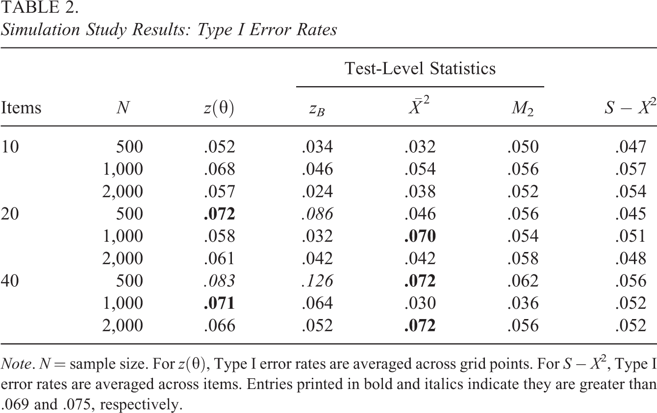
Based on 500 replications, the 95% confidence interval for rejection rates under the null with a .05 significance level is .031–.069. The corresponding interval based on Bradley’s (1978) liberal criteria is .025–.075. In Table 2, which presents Type I error rates, entries printed in bold and italics indicate they are greater than .069 and .075, respectively. In Tables 3 and 4, which present power, entries printed in bold and italics indicate the corresponding rates under the null are greater than .069 and .075, respectively. Such values should be interpreted with caution, given that the corresponding Type I error rates are inflated to some degree.

Table 2.

Simulation Study Results: Type I Error Rates

Items	N	$z (θ)$	Test-Level Statistics			S − X²
Items	N	$z (θ)$	z_B	${\bar{X}}^{2}$	M ₂	S − X²
10	500	.052	.034	.032	.050	.047
	1,000	.068	.046	.054	.056	.057
	2,000	.057	.024	.038	.052	.054
20	500	.072	.086	.046	.056	.045
	1,000	.058	.032	.070	.054	.051
	2,000	.061	.042	.042	.058	.048
40	500	.083	.126	.072	.062	.056
	1,000	.071	.064	.030	.036	.052
	2,000	.066	.052	.072	.056	.052

Note. N $=$ sample size. For $z (θ)$ , Type I error rates are averaged across grid points. For S − X², Type I error rates are averaged across items. Entries printed in bold and italics indicate they are greater than .069 and .075, respectively.

Table 3.

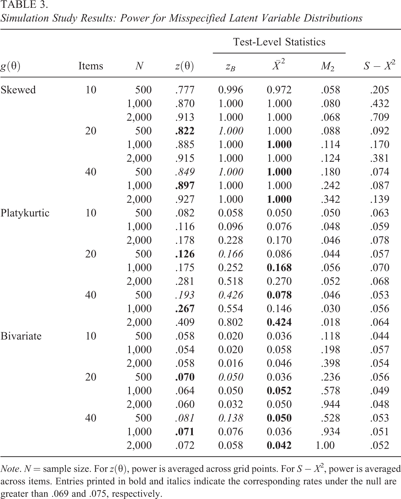
Simulation Study Results: Power for Misspecified Latent Variable Distributions

$g (θ)$	Items	N	$z (θ)$	Test-Level Statistics			S − X²
$g (θ)$	Items	N	$z (θ)$	z_B	${\bar{X}}^{2}$	M ₂	S − X²
Skewed	10	500	.777	0.996	0.972	.058	.205
		1,000	.870	1.000	1.000	.080	.432
		2,000	.913	1.000	1.000	.068	.709
	20	500	.822	1.000	1.000	.088	.092
		1,000	.885	1.000	1.000	.114	.170
		2,000	.915	1.000	1.000	.124	.381
	40	500	.849	1.000	1.000	.180	.074
		1,000	.897	1.000	1.000	.242	.087
		2,000	.927	1.000	1.000	.342	.139
Platykurtic	10	500	.082	0.058	0.050	.050	.063
		1,000	.116	0.096	0.076	.048	.059
		2,000	.178	0.228	0.170	.046	.078
	20	500	.126	0.166	0.086	.044	.057
		1,000	.175	0.252	0.168	.056	.070
		2,000	.281	0.518	0.270	.052	.068
	40	500	.193	0.426	0.078	.046	.053
		1,000	.267	0.554	0.146	.030	.056
		2,000	.409	0.802	0.424	.018	.064
Bivariate	10	500	.058	0.020	0.036	.118	.044
		1,000	.054	0.020	0.058	.198	.057
		2,000	.058	0.016	0.046	.398	.054
	20	500	.070	0.050	0.036	.236	.056
		1,000	.064	0.050	0.052	.578	.049
		2,000	.060	0.032	0.050	.944	.048
	40	500	.081	0.138	0.050	.528	.053
		1,000	.071	0.076	0.036	.934	.051
		2,000	.072	0.058	0.042	1.00	.052

Note. N $=$ sample size. For $z (θ)$ , power is averaged across grid points. For S − X², power is averaged across items. Entries printed in bold and italics indicate the corresponding rates under the null are greater than .069 and .075, respectively.

Table 4.

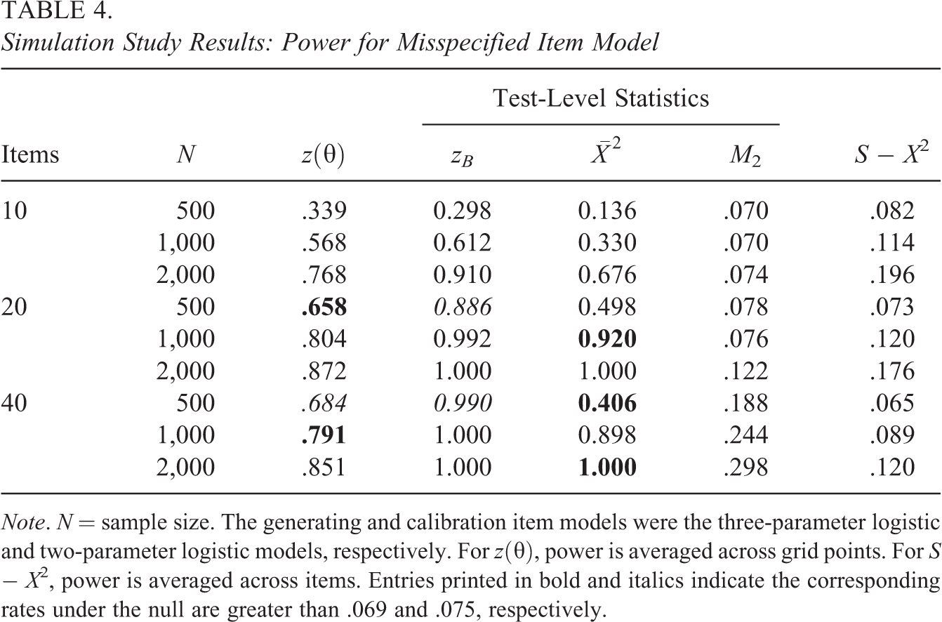
Simulation Study Results: Power for Misspecified Item Model

Items	N	$z (θ)$	Test-Level Statistics			S − X²
Items	N	$z (θ)$	z_B	${\bar{X}}^{2}$	M ₂	S − X²
10	500	.339	0.298	0.136	.070	.082
	1,000	.568	0.612	0.330	.070	.114
	2,000	.768	0.910	0.676	.074	.196
20	500	.658	0.886	0.498	.078	.073
	1,000	.804	0.992	0.920	.076	.120
	2,000	.872	1.000	1.000	.122	.176
40	500	.684	0.990	0.406	.188	.065
	1,000	.791	1.000	0.898	.244	.089
	2,000	.851	1.000	1.000	.298	.120

Note. N $=$ sample size. The generating and calibration item models were the three-parameter logistic and two-parameter logistic models, respectively. For $z (θ)$ , power is averaged across grid points. For S − X², power is averaged across items. Entries printed in bold and italics indicate the corresponding rates under the null are greater than .069 and .075, respectively.

For these results, the z_B, ${\bar{X}}^{2}$ , and M₂ statistics are directly comparable in the sense that they are all test-level statistics. In contrast, $z (θ)$ and S − X² are not test-level statistics. In the presented results, these statistics were simply averaged over grid points and items, respectively. These averages are of interest as they can be directly compared to their reference distributions.

Null condition

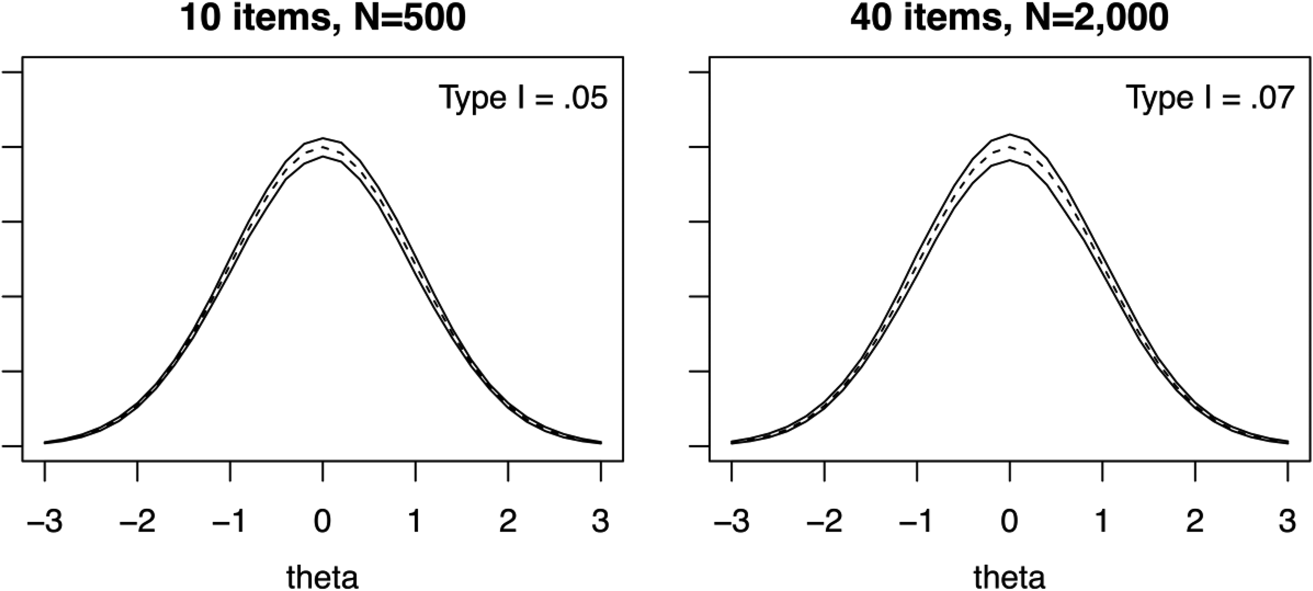
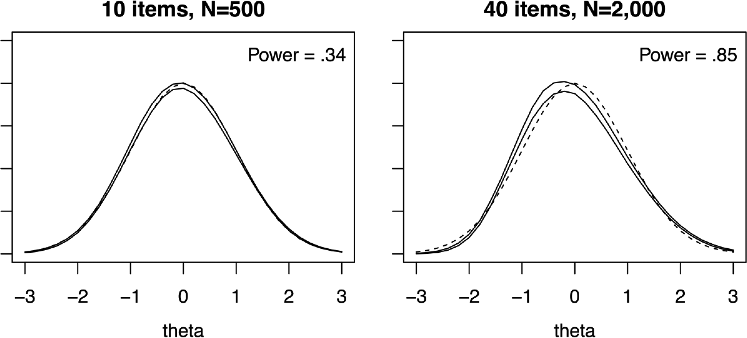
Table 2 presents Type I error rates under the null condition. For the proposed $z (θ)$ , a few of the rates are slightly liberal, mostly for combinations of smaller sample sizes and longer tests. For example, the greatest rate of .083 corresponds to the 40-item test with $N = 500$ . The results for $z (θ)$ may also be evaluated graphically. Figure 3 shows pointwise 90% empirical confidence intervals for the average posteriors $\bar{f} (θ| y; \hat{ω})$ across replications for the 10-item, $N = 500$ (left plot), and 40-item, $N = 2,000$ (right plot) combinations (i.e., the smallest and largest combinations). Note that this is an empirical confidence interval, which represents variability across replications, as opposed to the standard error–based confidence interval in Figure 1, which represents uncertainty for a single analysis. Both plots show that the pointwise empirical confidence intervals span $g (θ)$ and that the Monte Carlo variability is greater for central values of $θ$ .

Figure 3.

Posterior distribution 90% confidence intervals for z(θ) for the null condition (solid lines) and normal distribution (dashed line). Note. Type I error rates are averaged across all grid points and replications. Pointwise confidence intervals created by finding the 5th and 95th percentiles of $\bar{f} (θ | y; \hat{ω})$ across replications for each grid point.

For z_B, most of the rates are either well-controlled or conservative. However, with the smallest sample size, the rates for both the 20-item (.086) and 40-item (.126) tests are liberal. We found that with these combinations of conditions, $z (θ)$ tended to be overdispersed (i.e., had empirical variances greater than one) for larger absolute values of $θ$ . That is, for these values of $θ$ , the rate of convergence of $z (θ)$ was relatively slow, which affected the performance of z_B. Turning to the other two test-level statistics, the Type I error rates for both ${\bar{X}}^{2}$ and M₂ were well-controlled overall and consistent with previous studies (Li & Cai, 2018; Maydeu-Olivares & Joe, 2006). Finally, the rates for the item-level S − X² were similarly well-controlled.

Misspecified latent variable distribution

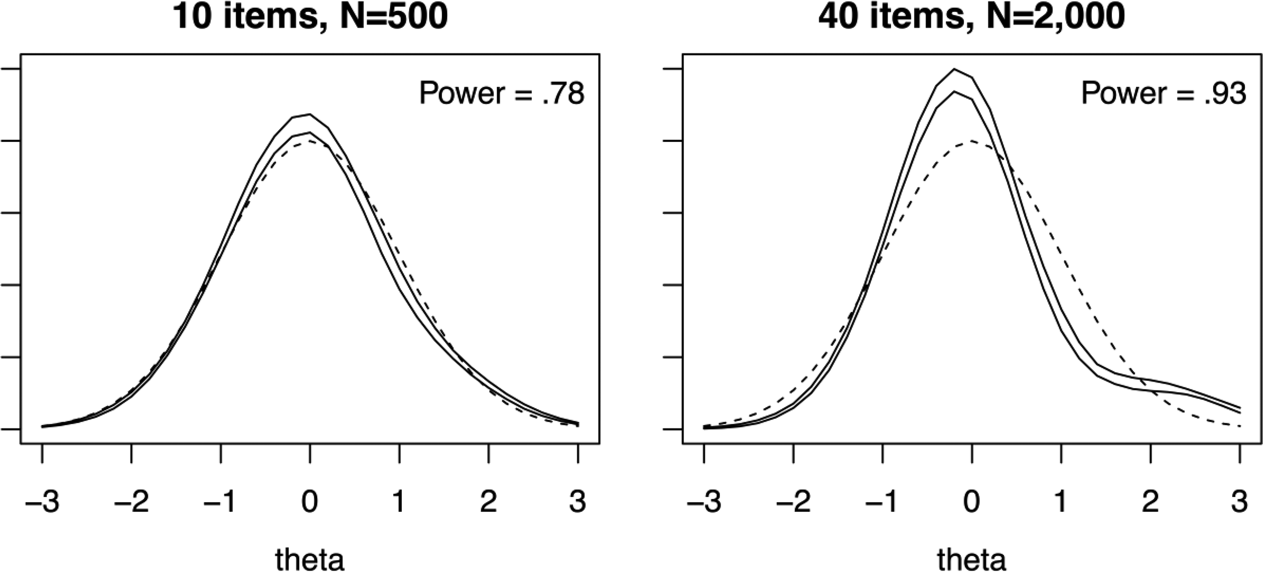
Table 3 presents power under misspecification of $g (θ)$ . For the skewed distribution, $z (θ)$ has high power, with all values exceeding .75. Figure 4 is analogous to Figure 3 and displays 90% confidence intervals for $\bar{f} (θ| y; \hat{ω})$ . The plot for the 40-item, $N = 2, 000$ combination shows that $\bar{f} (θ| y; \hat{ω})$ tends to resemble the generating skewed $g (θ)$ as the test length and sample size increase. The plot also demonstrates that even with substantial misspecification of $g (θ)$ , the power of $z (θ)$ , averaged across quadrature points, will likely be less than 1.0. This is because $\bar{f} (θ| y; \hat{ω}) = g (θ)$ for some values of $θ$ , and at these values, $z (θ)$ will not be statistically significant (e.g., see Figure 1). For both z_B and ${\bar{X}}^{2}$ , the power is 1.0 for all conditions except for the 10-item, $N = 500$ combination. This particular misspecification appears to be quite large, as both M₂ and $S - X^{2}$ have modest power. For example, for the 20-item, $N = 2, 000$ combination, the power for M₂ is .13 and the power for $S - X^{2}$ is .41. Previous studies have found M₂ generally lacks power to detect nonnormal $g (θ)$ (Li & Cai, 2018), and to our knowledge, $S - X^{2}$ has never been studied under misspecification of $g (θ)$ . For $S - X^{2}$ , the power is highest for the 10-item conditions, which is when summed scores probabilities will be most affected by the misspecification of $g (θ)$ .

Figure 4.

Posterior distribution 90% confidence intervals for z(θ) for the alternative skewed distribution condition (solid lines) and normal distribution (dashed line). Note. Power is averaged across all grid points and replications. Pointwise confidence intervals are created by finding the 5th and 95th percentiles of $\bar{f} (θ | y; \hat{ω})$ across replications for each grid point.

For the platykurtic distribution, Table 3 shows that $z (θ)$ has low-to-moderate power, with power increasing for longer tests and larger sample sizes. Figure 5 displays 90% confidence intervals for $\bar{f} (θ| y; \hat{ω})$ for this condition and is similar to Figure 4 in that for the 40-item, $N = 2, 000$ combination, $\bar{f} (θ| y; \hat{ω})$ begins to resemble the generating $g (θ)$ (see Figure 2). Turning to the test-level statistics, for z_B and ${\bar{X}}^{2}$ , the power increases with both sample size and test length. Notably, for the 20- and 40-item test lengths, the power of z_B is approximately double that of ${\bar{X}}^{2}$ . In contrast, M₂ has little power to detect this alternative condition, and the same is true for $S - X^{2}$ at the item level.

Figure 5.

Posterior distribution 90% confidence intervals for z(θ) for the alternative platykurtic distribution condition (solid lines) and normal distribution (dashed line). Note. Power is averaged across all grid points and replications. Pointwise confidence intervals are created by finding the 5th and 95th percentiles of $\bar{f} (θ | y; \hat{ω})$ across replications for each grid point.

For the bivariate distribution, Table 3 shows that $z (θ)$ has little power to detect the multidimensionality. Because of this lack of power, the plots of 90% confidence intervals for $\bar{f} (θ| y; \hat{ω})$ appear nearly identical to those under the null condition (see Figure 3) and are therefore not presented. As for the test-level statistics, z_B and ${\bar{X}}^{2}$ lack power to detect the multidimensionality, whereas M₂ has high power rates for this condition. These results for ${\bar{X}}^{2}$ and M₂ are consistent with those of Li and Cai (2018). Finally, the item-specific $S - X^{2}$ lacks power to detect the multidimensionality of $g (θ)$ .

Misspecified item model

Table 4 presents power when $g (θ)$ is correctly specified, but a 2PL model is fit to data generated using a 3PL model. Perhaps surprisingly, $z (θ)$ has moderate-to-high power, and these results support the conjecture that $z (θ)$ may be sensitive to item misfit at the test level. Also, Figure 6 shows how the misspecification manifests itself in $\bar{f} (θ| y; \hat{ω})$ . For the 10-item, $N = 500$ combination, the $\bar{f} (θ| y; \hat{ω})$ estimates appear very similar to a normal distribution. However, for the 40-item, $N = 2, 000$ combination, the posterior estimates tend to be right-skewed and exhibit a lack of fit across $θ$ values.

Figure 6.

Posterior distribution 90% confidence intervals for z(θ) for the alternative three-parameter logistic item model condition (solid lines) and normal distribution (dashed line). Note. Power is averaged across all grid points and replications. Pointwise confidence intervals are created by finding the 5th and 95th percentiles of $\bar{f} (θ | y; \hat{ω})$ across replications for each grid point.

For the test-level statistics, both z_B and ${\bar{X}}^{2}$ are relatively powerful in detecting this misspecification. Between the two, z_B is more powerful, in particular for the 10-item test length. It is also more powerful for the longer test lengths, but caution in interpretation is warranted because of a few inflated Type I error rates under the null for each statistic. As for M₂, it has low-to-moderate power, which is consistent with prior research (Hong et al., in press). Similarly, prior research has found $S - X^{2}$ to have low-to-moderate power in detecting this form of misspecification, which is consistent with the results in Table 4.

Empirical Examples

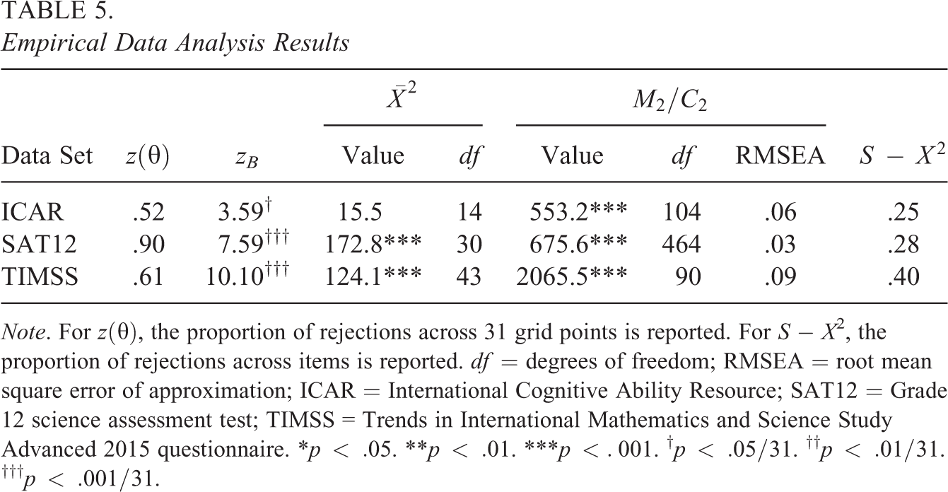
Three data sets were analyzed to illustrate the use of $z (θ)$ , the corresponding latent variable distribution fit plots, and z_B. The fit plots for the first two analyses are those presented earlier in Figure 1. For each example, a unidimensional model with a standard normal $g (θ)$ was used. For the first two examples, a 2PL model was used. For the third example, the data were ordinal, and a graded response model (Samejima, 1969) was used. Although not covered in the Methodological Background section, $z (θ)$ can be used with any standard unidimensional IRT model by redefining the conditional response probability in Equations 1 and 2. Also, for the third example, because the data were ordinal, the C₂ statistic (Monroe & Cai, 2015) was used instead of M₂. Otherwise, the same fit statistics used in the simulation study were calculated and are presented in Table 5. For completeness, the rejection rates for $S - X^{2}$ are included; however, as the focus of the examples is the fit of $g (θ)$ and overall fit, the $S - X^{2}$ results are not discussed further.

Table 5.

Empirical Data Analysis Results

Data Set	$z (θ)$	z_B	${\bar{X}}^{2}$		$M_{2} / C_{2}$			$S - X^{2}$
Data Set	$z (θ)$	z_B	Value	df	Value	df	RMSEA	$S - X^{2}$
ICAR	.52	3.59^†	15.5	14	553.2***	104	.06	.25
SAT12	.90	7.59^†††	172.8***	30	675.6***	464	.03	.28
TIMSS	.61	10.10^†††	124.1***	43	2065.5***	90	.09	.40

Note. For $z (θ)$ , the proportion of rejections across 31 grid points is reported. For S − X², the proportion of rejections across items is reported. $d f =$ degrees of freedom; RMSEA $=$ root mean square error of approximation; ICAR = International Cognitive Ability Resource; SAT12 = Grade 12 science assessment test; TIMSS = Trends in International Mathematics and Science Study Advanced 2015 questionnaire. * $p < .05$ . ** $p < .01$ . *** $p < . 001$ . ^† $p < .05 / 31$ . ^†† $p < .01 / 31$ . ^††† $p < .001 / 31$ .

International Cognitive Ability Resource (ICAR) Example

The first data set comprises 16 dichotomously scored items, representing four subdomains, from the International Cognitive Ability Resource (ICAR; Condon & Revelle, 2014) measure. The ICAR data were obtained from the psych package (Revelle, 2017) for R, and for convenience, only the $N = 1,248$ complete cases were analyzed. Table 5 shows that the maximum absolute value of $z (θ)$ is just $z_{B} = 3.59$ ( $p < .05 / 31$ ), despite the moderately large sample size, and ${\bar{X}}^{2} = 15.5$ is not significant ( $d f = 14$ , $p = .35$ ). Also, returning to Figure 1, the $g (θ)$ fit plot (top panel) does not show obvious misfit. In contrast, M₂ is significant (553.2, $d f = 104$ , $p < .001$ ) and the corresponding root mean square error of approximation (RMSEA) value (.06) suggests acceptable, but not close, fit (Maydeu-Olivares & Joe, 2014; see also Monroe & Cai, 2015). Based on the simulation study findings that M₂ is sensitive to unmodeled latent dimensions, and the intended multidimensional structure of the assessment (Condon & Revelle, 2014), the fit statistics may be interpreted as suggesting that a multidimensional IRT model may be more appropriate for this data set. Furthermore, the specification of a normal $g (θ)$ and the 2PL model appear to be appropriate, given z_B and the fit plot.

Grade 12 Science Assessment Test (SAT12) Example

The second data set is from a Grade 12 science assessment test (SAT12) made available in the TESTFACT manual (Wood et al., 2003) and has been analyzed in previous IRT research (Chalmers et al., 2017; Monroe, 2019). There are 32 dichotomously scored items, and $N = 572$ complete cases were analyzed. Table 5 shows that, in contrast to the ICAR analysis results, both z_B (7.59, $p < .001 / 31$ ) and ${\bar{X}}^{2}$ (172.8, $d f = 30$ , $p < .001$ ) suggest poor fit. This conclusion is supported by the $g (θ)$ fit plot in Figure 1 (bottom panel), which shows a right-skewed average posterior $\bar{f} (θ| y; \hat{ω})$ . In contrast, the RMSEA value (.03) suggests close fit. Again, based on the simulation study findings, the fit statistics may be interpreted as suggesting either the normal distribution assumption for $g (θ)$ is suspect or that a more flexible item model (e.g., the 3PL model) may be more appropriate. However, the specification of a unidimensional model appears defensible, given the M₂-based RMSEA.

TIMSS Advanced 2015 Questionnaire Example

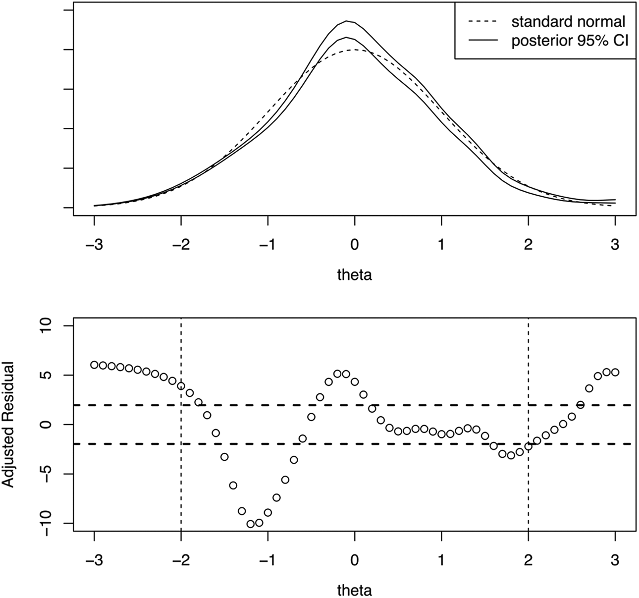
The third data set is from a questionnaire given to Trends in International Mathematics and Science Study (TIMSS) Advanced 2015 (Martin et al., 2016) students on their views of engaging teaching in advanced mathematics. There are 15 Likert-type items, each with four response categories, and $N = 2, 856$ complete cases from the United States were analyzed. Table 5 shows that the model provides poor fit as judged by z_B (10.10, $p < .001 / 31$ ) and ${\bar{X}}^{2}$ (124.1, $d f = 41$ , $p < .001$ ). Figure 7 presents a $g (θ)$ fit plot (top panel), which shows that $\bar{f} (θ| y; \hat{ω})$ is highly peaked in comparison to the normal distribution, and the model provides poor fit for central and negative values of $θ$ . Also, Figure 7 provides a plot of $z (θ)$ (bottom panel), analogous to plots of item-fit residuals (Haberman et al., 2013). The plot of $z (θ)$ confirms that the model fits poorly for central and negative values of $θ$ . In addition, the C₂-based RMSEA (.09) suggests there may be residual associations among the items not accounted for by the model.

Figure 7.

Latent variable distribution fit plot (top) and corresponding z(θ) residual plot (bottom) for TIMMS Advanced Questionnaire data. Note. Results from fitting graded response model to TIMSS Advanced Questionnaire data on students’ view of engaging teaching in advanced mathematics. Horizontal dashed lines correspond to critical values for z(θ) at .05 significance level.

Conclusion

In this research, a statistic for examining the fit of the latent variable distribution in unidimensional IRT was proposed. Due to a fundamental relationship between the latent variable distribution and individual posterior distributions, this statistic, $z (θ)$ , falls within the generalized residuals framework proposed by Haberman and Sinharay (2013). Consequently, it enjoys an asymptotic standard normal distribution. Further, the statistic conditions on a fixed value of $θ$ and can be considered complementary to residual-based item-fit statistics (e.g., Haberman et al., 2013). The overall (i.e., unconditional) fit of the latent variable distribution can also be tested using the Bonferroni-corrected z_B.

The simulation study demonstrated that under the null, $z (θ)$ appears reasonably well-calibrated across a range of test lengths and sample sizes, and all Type I error rates were below .09. This is notable as the related residual-based item statistic of Haberman et al. (2013) requires larger sample sizes to attain satisfactory performance under the null. Under arguably comparable simulation conditions in Haberman et al. (2013), the Type I error rates for the item-fit statistics for various model sizes with $N = 500$ are all at least .10 (see Table 2). This difference in performance is likely due to $z (θ)$ being based on more information: Tests of latent variable distribution fit focus on responses for all items (either through posteriors or summed scores), whereas tests of item fit must necessarily focus on responses for a single item. As for z_B, the Type I error rates were conservative or well-controlled for all conditions except for the smallest sample size ( $N = 500$ ) combined with the 20-item and 40-item tests.

The simulation study also demonstrated that under the studied alternative conditions, the results for $z (θ)$ and z_B are largely consistent with those for ${\bar{X}}^{2}$ . These statistics all had high power to detect the skewed $g (θ)$ and little power to detect the bivariate $g (θ)$ . Between z_B and ${\bar{X}}^{2}$ , the former had higher power to detect the platykurtic $g (θ)$ . Also, as test length and sample size increase, the average posterior $\bar{f} (θ| y; \hat{ω})$ begins to resemble the data-generating distribution, even under misspecification. Interestingly, the simulation study results showed that $z (θ)$ , z_B, and ${\bar{X}}^{2}$ are sensitive to misspecification of the item model at the test level.

The empirical data examples demonstrated how the proposed statistics might be used in practice. In particular, the suggested $g (θ)$ fit plots can provide an intuitive picture for evaluating the latent variable distribution fit. Further, if the z_B is not significant, then it cannot be used to conclude the specified latent variable distribution or item models fit the data poorly. As such, z_B can be useful to practitioners in collecting evidence regarding the fit of an IRT model (American Educational Research Association, American Psychological Association, & National Council for Measurement in Education, 2014). If, however, z_B is significant, the interpretation is less straightforward, given that it is sensitive to both misfit of $g (θ)$ and misfit of the item models. For example, with the SAT12 empirical example, for the fitted model specifying normal $g (θ)$ and 2PL, $z_{B} = 7.59$ ( $p < .001 / 31$ ). How, then, should a researcher revise the model? We argue that in such cases, model revision should be guided by theoretical plausibility and practical convenience, while still prioritizing model parsimony (Pitt & Myung, 2002). For example, if the researcher knows that two subpopulations are included in the sample, specifying a more flexible model for $g (θ)$ would be sensible. Alternatively, if the researcher believes that guessing was widely used as a test-taking strategy, specifying a 3PL would be defensible. With either approach, it is likely that model fit would improve as judged by z_B.

There are numerous directions for future research. First, the proposed statistic can be extended to multidimensional IRT models. For bifactor models (Gibbons & Hedeker, 1992), $z (θ)$ and z_B could be used to evaluate the fit of the distribution for the general factor. For correlated-factors models, however, such an extension would only be practical with a small number of latent dimensions, as the total number of quadrature points grows exponentially with the latent dimensionality. Second, following van Rijn et al. (2016), the proposed statistic can be applied for use in large-scale educational assessments (e.g., NAEP). Third, additional simulation work can be carried out to evaluate the performance of $z (θ)$ and z_B under other conditions. In particular, shorter tests and smaller sample sizes could be considered to better understand the limitations of the statistic under the null. And, other types of $g (θ)$ misspecification (e.g., bimodal distributions) and item model misspecification (Sinharay, 2006) should be studied to better understand the power of $z (θ)$ under such conditions. Fourth, it would be helpful to develop a goodness-of-fit index based on z_B, analogous to the RMSEA fit index based on M₂ (Maydeu-Olivares & Joe, 2014). Fifth, further research can be conducted on how $z (θ)$ can be used in practice. The empirical examples demonstrated how practitioners could use $z (θ)$ , along with other goodness-of-fit measures, to identify potential deficiencies in the specified IRT model. But, more work along these lines could result in guidelines for practitioners. Finally, related to the fifth future direction, research can further study the practical significance of latent variable distribution misfit (Sinharay & Haberman, 2014). For example, Woods (2006) studies the effect of $g (θ)$ misfit on EAP scores, but more work along these lines is needed.

Footnotes

Declaration of Conflicting Interests

The author(s) declared no potential conflicts of interest with respect to the research, authorship, and/or publication of this article.

Funding

The author(s) received no financial support for the research, authorship, and/or publication of this article.

Notes

References

Adams

R. J.

Wilson

Wang

W. C.

(1997). The multidimensional random coefficients multinomial logit model. Applied Psychological Measurement, 21(1), 1–23.

American Educational Research Association, American Psychological Association, & National Council on Measurement in Education. (2014). Standards for educational and psychological testing. American Educational Research Association.

Béguin

A. A.

Glas

C. A.

(2001). MCMC estimation and some model-fit analysis of multidimensional IRT models. Psychometrika, 66(4), 541–561.

Birnbaum

A. L.

(1968). Some latent trait models and their use in inferring an examinee’s ability. In Lord

F. M.

Novick

M. R.

(Eds.), Statistical theories of mental test scores (pp. 397–479). Addison-Wesley.

Bock

R. D.

Aitkin

(1981). Marginal maximum likelihood estimation of item parameters: Application of an EM algorithm. Psychometrika, 46(4), 443–459.

Bradley

J. V.

(1978). Robustness? British Journal of Mathematical and Statistical Psychology, 31(2), 144–152.

Cai

(2017). flexMIRT version 3.51: Flexible multilevel multidimensional item analysis and test scoring [Computer software]. Vector Psychometric Group.

Chalmers

R. P.

Pek

Liu

(2017). Profile-likelihood confidence intervals in item response theory models. Multivariate Behavioral Research, 52(5), 533–550.

Condon

D. M.

Revelle

(2014). The international cognitive ability resource: Development and initial validation of a public-domain measure. Intelligence, 43, 52–64.

10.

du Toit

(Ed.). (2003). IRT from SSI. Lincolnwood: Scientific Software International.

11.

Ferrando

P. J.

Lorenzo-Seva

(2001). Checking the appropriateness of item response theory models by predicting the distribution of observed scores: The program EO-Fit. Educational and Psychological Measurement, 61(5), 895–902.

12.

Gibbons

R. D.

Hedeker

D. R.

(1992). Full-information item bi-factor analysis. Psychometrika, 57(3), 423–436.

13.

Haberman

S. J.

(2009). Use of generalized residuals to examine goodness of fit of item response models (ETS Research Report No. RR-09-15). Educational Testing Service.

14.

Haberman

S. J.

Sinharay

(2013). Generalized residuals for general models for contingency tables with application to item response theory. Journal of the American Statistical Association, 108(504), 1435–1444.

15.

Haberman

S. J.

Sinharay

Chon

K. H.

(2013). Assessing item fit for unidimensional item response theory models using residuals from estimated item response functions. Psychometrika, 78(3), 417–440.

16.

Hambleton

R. K.

Swaminathan

(1985). Item response theory: Principles and applications. Kluwer Academic.

17.

Hong

S. E.

Monroe

Falk

C. F.

(in press). Performance of person-fit statistics under model misspecification. Journal of Educational Measurement.

18.

E. H.

(2010). Interpretation of the three-parameter testlet response model and information function. Applied Psychological Measurement, 34(7), 467–482.

19.

Köhler

Robitzsch

Hartig

(2020). A bias-corrected RMSD item fit statistic: An evaluation and comparison to alternatives. Journal of Educational and Behavioral Statistics, 45(3), 251–273.

20.

Cai

(2018). Summed score likelihood–based indices for testing latent variable distribution fit in item response theory. Educational and Psychological Measurement, 78(5), 857–886.

21.

Louis

T. A.

(1982). Finding the observed information matrix when using the EM algorithm. Journal of the Royal Statistical Society: Series B, 44, 226–233.

22.

Martin

M. O.

Mullis

I. V. S.

Hooper

Yin

Foy

Palazzo

(2016). Creating and Interpreting the TIMSS Advanced 2015 Context Questionnaire Scales. In Martin

M. O.

Mullis

I. V. S.

Hooper

(Eds.), Methods and procedures in TIMSS Advanced 2015 (pp. 15.1–15.73). TIMSS & PIRLS International Study Center, Boston College. https://timssandpirls.bc.edu/publications/timss/2015-a-methods/chapter-15.html

23.

Maydeu-Olivares

Joe

(2006). Limited information goodness-of-fit testing in multidimensional contingency tables. Psychometrika, 71(4), 713.

24.

Maydeu-Olivares

Joe

(2014). Assessing approximate fit in categorical data analysis. Multivariate Behavioral Research, 49(4), 305–328.

25.

Meilijson

(1989). A fast improvement to the EM algorithm on its own terms. Journal of the Royal Statistical Society: Series B, 51, 127–138.

26.

Mislevy

R. J.

(1984). Estimating latent distributions. Psychometrika, 49(3), 359–381.

27.

Monroe

(2019). Estimation of expected Fisher information for IRT models. Journal of Educational and Behavioral Statistics, 44(4), 431–447.

28.

Monroe

Cai

(2014). Estimation of a Ramsay-curve item response theory model by the Metropolis–Hastings Robbins–Monro algorithm. Educational and Psychological Measurement, 74(2), 343–369.

29.

Monroe

Cai

(2015). Evaluating structural equation models for categorical outcomes: A new test statistic and a practical challenge of interpretation. Multivariate Behavioral Research, 50(6), 569–583.

30.

Muraki

Bock

R. D.

(2003). PARSCALE 4.1. Scientific Software International.

31.

Orlando

Thissen

(2000). Likelihood-based item-fit indices for dichotomous item response theory models. Applied Psychological Measurement, 24(1), 50–64.

32.

Pitt

M. A.

Myung

I. J.

(2002). When a good fit can be bad. Trends in Cognitive Sciences, 6(10), 421–425.

33.

R Core Team. (2018). R: A language and environment for statistical computing. R Foundation for Statistical Computing. https://www.R-project.org/

34.

Reise

S. P.

Rodriguez

Spritzer

K. L.

Hays

R. D.

(2018). Alternative approaches to addressing non-normal distributions in the application of IRT models to personality measures. Journal of Personality Assessment, 100(4), 363–374.

35.

Revelle

W. R.

(2017). psych: Procedures for personality and psychological research [Computer software manual]. http://cran.r-project.org/web/packages/psych/. (R package version 1.7.8).

36.

Samejima

(1969). Estimation of latent ability using a response pattern of graded scores (Psychometrika Monograph Supplement No. 17). Psychometric Society.

37.

Satorra

Bentler

P. M.

(1994). Corrections to test statistics and standard errors in covariance structure analysis. In von Eye

Clogg

C. C.

(Eds.), Latent variables analysis: Applications for developmental research (pp. 399–419). Sage.

38.

Sinharay

(2006). Bayesian item fit analysis for unidimensional item response theory models. British Journal of Mathematical and Statistical Psychology, 59(2), 429–449.

39.

Sinharay

Haberman

S. J.

(2014). How often is the misfit of item response theory models practically significant?. Educational Measurement: Issues and Practice, 33(1), 23–35.

40.

Sinharay

Johnson

M. S.

Stern

H. S.

(2006). Posterior predictive assessment of item response theory models. Applied Psychological Measurement, 30(4), 298–321.

41.

Sireci

S. G.

Thissen

Wainer

(1991). On the reliability of testlet-based tests. Journal of Educational Measurement, 28(3), 237–247.

42.

Thissen

(2013). Using the testlet response model as a shortcut to multidimensional item response theory subscore computation. In Millsap

van der Ark

Bolt

Woods

(Eds.), New developments in quantitative psychology—Presentations from the 77th Annual Psychometric Society Meeting (pp. 29–40). Springer.

43.

van Rijn

P. W.

Sinharay

Haberman

S. J.

Johnson

M. S.

(2016). Assessment of fit of item response theory models used in large-scale educational survey assessments. Large-Scale Assessments in Education, 4(1), 10.

44.

Wells

C. S.

Hambleton

R. K.

(2016). Model fit with residual analyses. In van der Linden

W. J.

(Ed.), Handbook of item response theory (Vol. 2, pp. 395–413). CRC Press.

45.

Wood

Wilson

D. T.

Muraki

Schilling

S. G.

Gibbons

Bock

R. D.

(2003). TESTFACT 4: Test scoring, item statistics, and item factor analysis (Version 4). Scientific Software International.

46.

Woods

C. M.

(2006). Ramsay-curve item response theory (RC-IRT) to detect and correct for nonnormal latent variables. Psychological Methods, 11(3), 253.

47.

Woods

C. M.

Lin

(2009). Item response theory with estimation of the latent density using Davidian curves. Applied Psychological Measurement, 33(2), 102–117.

48.

Woods

C. M.

Thissen

(2006). Item response theory with estimation of the latent population distribution using spline-based densities. Psychometrika, 71(2), 281.