Regression Discontinuity Designs With an Ordinal Running Variable: Evaluating the Effects of Extended Time Accommodations for English-Language Learners

Abstract

Regression discontinuity (RD) designs are commonly used for program evaluation with continuous treatment assignment variables. But in practice, treatment assignment is frequently based on ordinal variables. In this study, we propose an RD design with an ordinal running variable to assess the effects of extended time accommodations (ETA) for English-language learners (ELLs). ETA eligibility is determined by ordinal ELL English-proficiency categories of National Assessment of Educational Progress data. We discuss the identification and estimation of the average treatment effect (ATE), intent-to-treat effect, and the local ATE at the cutoff. We also propose a series of sensitivity analyses to probe the effect estimates’ robustness to the choices of scaling functions and cutoff scores and remaining confounding.

Keywords

regression discontinuity designs causal inference testing accommodations NAEP observational studies

1. Introduction

In educational assessment, there have been ongoing efforts to include English-language learners (ELLs) and students with disabilities (SDs) in the National Assessment of Educational Progress (NAEP) assessment by providing appropriate testing accommodations (National Research Council, 2002). Among various testing accommodations, the extended time accommodation (ETA) is the most frequently offered accommodation in the NAEP assessment and other testing programs (Gregg & Nelson, 2012); the recent 2017 NAEP assessment included about 90% of ELLs and SD students, and about 10% of these students received ETA (National Center for Education Statistics [NCES], 2017a, 2017b). Despite the common usage of ETA, there is little guidance on how to evaluate ETA and no systematic research studies assessing ETA’s effectiveness (Jonson et al., 2019). Given that it is unethical and impractical to conduct a randomized experiment in this setting, the goal of this article is to propose a regression discontinuity (RD) design with an ordinal running variable for evaluating program effectiveness.

RD designs have been used for policy and program evaluation where subjects’ treatment status is determined by whether their treatment assignment variable (also called running or forcing variable) exceeds a predefined cutoff. If the running variable is continuous, as required by standard RD designs, the average treatment effect (ATE) at the cutoff is nonparametrically identified and can be estimated by comparing the average outcomes of subjects “just below” and “just above” the cutoff (Hahn et al., 2001; Imbens & Lemieux, 2008; Lee & Lemieux, 2010). However, in some settings, the running variable is discrete, reported in coarse intervals, or an ordinal variable with a few categories only. For instance, in NAEP assessments, student eligibility for ETA is determined by ELL English-proficiency scores, an ordinal variable with six categories: No Proficiency, ELL Beginning, ELL Intermediate, ELL Advanced, Formerly ELL, and Never ELL. Students with ELL Advanced (here, the cutoff) or lower proficiency level are offered ETA. Due to the running variable’s discrete and ordinal scale, the ATE at the cutoff is no longer nonparametrically identified because in the close vicinity of the cutoff score only ETA eligible students are observed (i.e., there is no overlap of eligible and ineligible students even in the limit at the cutoff). Thus, the identification of the ATE at the cutoff requires an appropriate scaling of the ordinal categories together with a correctly specified parametric outcome model to extrapolate the average control outcome of ineligible ETA students to the cutoff category of ELL Advanced students.

In this article, we extend the identification and estimation strategy proposed by Lee and Card (2008) for discrete running variables to ordinal variables. With ordinal running variables, RD designs face several challenges: First, the categories of the ordinal running variable need to be mapped onto a numeric scale by choosing an appropriate scaling function. For instance, using the ranks {1,…, 6} is a possible but not necessarily the only choice for the six ELL English-proficiency categories above. Second, a meaningful cutoff score between ELL Advanced and Formerly ELL must be determined with respect to the chosen numeric scale. The choice of the cutoff score determines the target population (at the cutoff) as well as the magnitude of the ATE. Third, the parametric functional form to the left and the right of the cutoff score must be correctly specified with respect to the chosen numeric scale, such that extrapolations to the cutoff score are accurate. Fourth, the statistical uncertainty due to the discreteness of the scaled running variable should be accounted for when estimating standard errors (Lee & Card, 2008). Fifth, given the increased number of assumptions with ordinal running variables and the potential violation of these assumptions, we need to conduct a set of sensitivity analyses to strengthen causal conclusions drawn from the analysis. These include probing the effect estimate’s sensitivity to (i) the choice of the scaling function, (ii) the choice of the scaled cutoff score, and (iii) remaining confounding due to model misspecification (see Section 3 for details). We remark that there are other approaches that can accommodate ordinal or discrete running variables in RD designs, such as using propensity scores as a surrogate continuous running variable under the local randomization framework (Li et al., 2021) and linking analysis of covariance and local randomization heuristics (Sales & Hansen, 2020).

Throughout this article, we use the ETA example based on the 2017 NAEP data to demonstrate our proposed approach. We discuss some points that investigators should consider when choosing the scaling function and the cutoff score. We then analyze the intent-to-treat (ITT) and the local ATE (LATE) that accounts for noncompliance with respect to the assigned ETA status.

The remainder of this article is organized as follows. Section 2 briefly reviews the sharp and fuzzy RD framework with a continuous running variable. Section 3 discusses the assumptions required for RD designs with an ordinal running variable. Section 4 describes the analyses and results of our empirical example concerning the effects of ETA using the 2017 NAEP data for mathematics; this section also includes the aforementioned sensitivity analyses to the assumptions laid out in Section 3. Conclusions are given in Section 5.

2. Setup

2.1. Notation

We use the Neyman–Rubin potential outcomes framework (Neyman, 1923; Rubin, 1974) and its extension to multilevel/clustered data by Hong and Raudenbush (2006) to define treatment effects in sharp and fuzzy RD designs. The NAEP sampling design involves a multilevel structure, where students, the study units, are nested within schools. Let $A_{i j} \in {0, 1}$ be a binary treatment variable, where $A_{i j} = 1$ indicates that student i in school j was assigned to the ETA treatment and $A_{i j} = 0$ indicates the control condition. In a classic RD design, treatment assignment is based on a continuous running variable $X_{i j}$ and a cutoff score x_c , such that $A_{i j} = 1$ if $X_{i j} \leq x_{c}$ and $A_{i j} = 0$ if $X_{i j} > x_{c}$ . Let $Z_{i j} \in {0, 1}$ denote the treatment received, where $Z_{i j} = 1$ if student i in school j actually received ETA and $Z_{i j} = 0$ if the student did not receive ETA. Note, for a sharp RD design (without noncompliance), assignment status and treatment receipt are identical, that is, $A_{i j} = Z_{i j}$ .

$Y_{i j} (1)$ denotes the potential treatment outcome if student i in school j were to receive ETA, and $Y_{i j} (0)$ denotes the potential control outcome for the same student but under the control condition. For every student, the observed outcome is linked to the potential outcomes as follows: $Y_{i j} = Z_{i j} Y_{i j} (1) + (1 - Z_{i j}) Y_{i j} (0)$ . The equality implies the stable unit treatment value assumption (SUTVA; Rubin, 1986), that is, (1) a student’s potential outcomes are independent of other students’ treatment assignment and (2) there are no different versions of the treatment. Since ETA eligibility is unlikely to have spillover effects to other students and every school uses the same ETA (e.g., fixed amount of extra time), SUTVA is plausible in our study. SUTVA would be violated (i) if some students are aware of other students’ ETA eligibility status and this awareness creates negative (or positive) externalities on students’ performance and (ii) if the overall fraction of ETA eligible students affects performance of students in a school. Finally, let $W_{i j}$ be a set of observed pretreatment covariates and $U_{i j}$ be unobserved confounders.

2.2. Review: Sharp RD Designs With a Continuous Running Variable

We first review the standard sharp RD design with a continuous running variable. Suppose our running variable, ELL English proficiency, is continuous where students scoring below or at the cutoff, $X_{i j} \leq x_{c}$ , are eligible for ETA and students scoring above the cutoff are ineligible for ETA. Given full compliance with the assigned ETA status, this design is called a sharp RD design because the probability of receiving treatment jumps from one to zero when the running variable $X_{i j}$ crosses the cutoff x_c .

Because $A_{i j}$ is a known deterministic function of $X_{i j}$ , conditional unconfoundedness holds, that is, $Y_{i j} (1), Y_{i j} (0) ⊥ A_{i j} | X_{i j}$ . Nonetheless, the treatment effect for the entire population is nonparametrically not identified because the positivity assumption, which requires $0 < P r (A_{i j} = 1 | X_{i j}) < 1$ , is violated. In fact, in a sharp RD design, treatment and control units do not share any common support on $X_{i j}$ , such that $P r (A_{i j} = 1 | X_{i j} \leq x_{c}) = 1$ for every individual scoring below or at the cutoff and $P r (A_{i j} = 1 | X_{i j} > x_{c}) = 0$ for every individual scoring above the cutoff. But the treatment effect for the population at or in the close vicinity of the cutoff score is nonparametrically identified if the potential outcomes meet a local smoothness assumption at the limiting cutoff:

(A1) Local Continuity of Potential Outcomes:

lim_{x ↑ x_{c}} E (Y_{i j} (1) | X_{i j} = x) = lim_{x ↓ x_{c}} E (Y_{i j} (1) | X_{i j} = x)

lim_{x ↑ x_{c}} E (Y_{i j} (0) | X_{i j} = x) = lim_{x ↓ x_{c}} E (Y_{i j} (0) | X_{i j} = x)

This assumption states that the mean potential treatment and control outcomes right below the cutoff are equal to the corresponding mean potential outcomes right above the cutoff. The assumption allows us to think of an RD design as a local randomized experiment where students near the cutoff are randomly assigned to treatment and control conditions (Lee & Lemieux, 2010). Under (A1), the ATE at the cutoff, $τ (x_{c})$ , is identified as follows:

τ (x_{c}) = E [Y_{i j} (1) - Y_{i j} (0) | X_{i j} = x_{c}]

= lim_{x ↑ x_{c}} E (Y_{i j} | X_{i j} = x) - lim_{x ↓ x_{c}} E (Y_{i j} | X_{i j} = x) .

In our setting, the ATE at the cutoff represents the average effect of ETA for students scoring right at the eligibility cutoff. We can estimate $τ (x_{c})$ by comparing the average outcomes for students scoring “just below” and “just above” the cutoff using nonparametric, local polynomial regression. Baseline covariates $W_{i j}$ can be included to improve the efficiency of the estimated effect. For more details on sharp RD designs and the nonparametric estimation of treatment effects at the cutoff, see Imbens and Lemieux (2008) and Lee and Lemieux (2010).

2.3. Review: Fuzzy RD Designs With a Continuous Running Variable

In practice, study administrators frequently do not adhere to the assignment rules or participants do not comply with the assigned treatment or control status. For instance, students eligible for ETA according to their English-proficiency scores may not receive ETA and ineligible students might actually receive ETA due to school- or administrator-specific rules or exemptions. In the presence of noncompliance, we have a fuzzy RD design that can identify the ITT and LATE at the cutoff score. Using the ETA eligibility status, $A_{i j}$ , as the “treatment” indicator, the ITT at the cutoff is identifiable and estimable in the same way as the ATE in the sharp RD design of Section 2.2. Specifically, to define and formalize the identification of the LATE, we now use potential outcomes notations for treatment receipt. Let $Z_{i j} (1)$ be a student’s potential ETA receipt if she were eligible for ETA ( $A_{i j} = 1$ ) and $Z_{i j} (0)$ be the potential ETA receipt if she were not eligible for ETA ( $A_{i j} = 0$ ). We also assume $Z_{i j} = A_{i j} Z_{i j} (1) + (1 - A_{i j}) Z_{i j} (0)$ . Compared to the sharp RD design, the fuzzy RD design is characterized by a discontinuity in the treatment receipt probability of less than one but still requires a discontinuity greater than zero, that is, $0 < lim_{x ↑ x_{c}} P r (Z_{i j} = 1 | X_{i j} = x) - lim_{x ↓ x_{c}} P r (Z_{i j} = 1 | X_{i j} = x) < 1$ . Additionally, the fuzzy RD design needs the following two assumptions.

(A2) Local Monotonicity:

$lim_{x ↑ x_{c}} P r (Z_{i j} (1) < Z_{i j} (0) | X_{i j} = x) = lim_{x ↓ x_{c}} P r (Z_{i j} (1) < Z_{i j} (0) | X_{i j} = x) = 0.$

(A3) Local Exclusion Restriction:

$lim_{x ↑ x_{c}} P r (Y_{i j} (1, z) = Y_{i j} (0, z) | X_{i j} = x) = lim_{x ↓ x_{c}} P r (Y_{i j} (1, z) = Y_{i j} (0, z) | X_{i j} = x)$ for each $z = 0, 1$ , and where the potential outcomes $Y_{i j} (a, z)$ are now functions of both the assigned treatment status (a) and the received treatment status (z).

The local monotonicity assumption rules out the presence of defiers at the cutoff, that is, students who would receive ETA if not eligible for ETA but would not receive ETA if eligible. Assumptions (A1)–(A3) allow us to identify the ATE for the latent subpopulation of compliers at the cutoff, that is, students who would receive ETA if they were eligible for ETA and who would not receive ETA if ineligible (i.e., $Z_{i j} (1) = 1$ and $Z_{i j} (0) = 0$ ). The treatment effect for the “local” complier subpopulation is referred to as the LATE. The local exclusion restriction states that the potential outcomes depend only on treatment receipt ( $Z_{i j}$ ) but are unaffected by treatment assignment $A_{i j}$ at the limiting cutoff. With assumptions (A1)–(A3), the LATE at the cutoff is identified as follows.

τ_{LATE} (x_{c}) = E [Y_{i j} (1) - Y_{i j} (0) | X_{i j} = x_{c}, Z_{i j} (1) = 1, Z_{i j} (0) = 0]

= \frac{lim_{x ↑ x_{c}} E (Y_{i j} | X_{i j} = x) - lim_{x ↓ x_{c}} E (Y_{i j} | X_{i j} = x)}{lim_{x ↑ x_{c}} E (Z_{i j} | X_{i j} = x) - lim_{x ↓ x_{c}} E (Z_{i j} | X_{i j} = x)} .

In our study, $τ_{LATE} (x_{c})$ is the average effect of receiving ETA among complier students at the cutoff. We can estimate $τ_{LATE} (x_{c})$ by taking the ratio between the difference in the expected outcomes and the difference in the expected treatment receipt probabilities of students “just above” and “just below” the cutoff. Local polynomial regression is frequently used to estimate the numerator and denominator of the ratio. Also, similar to $τ (x_{c})$ , we can improve the efficiency of the estimator by using covariates $W_{i j}$ . For more details, see Imbens and Lemieux (2008) and Lee and Lemieux (2010).

2.4. Review: A Graphical Perspective

The data-generating process underlying RD designs can be formalized by a causal diagram—a directed acyclic graph (DAG; Elwert, 2013; Morgan & Winship, 2014; Pearl, 1988, 2009; Steiner et al., 2017). The DAG for the ETA evaluation is shown in Figure 1(a). The graph highlights that the ELL eligibility status (A) is solely determined by a student’s ELL English-proficiency score (X), while the ETA receipt status (Z) depends on the eligibility status (A) and on observed and unobserved covariate sets ( $W, U$ ). That is, school administrators might offer ETA to ineligible students or withhold ETA from eligible students based on variables captured by $W$ and $U$ . The set of measured covariates $W$ may include student background variables like the number of years exposed to English education or race/ethnicity. The set of unmeasured covariates $U$ may include students’ academic abilities/skills or the number of English-language books read per month. Since the covariate sets $W$ and $U$ also affect students’ outcome (Y), they confound the causal relation between ETA eligibility (A) and the outcome (Y) and the causal relation between ETA receipt (Z) and the outcome (Y). Thus, without covariate adjustments, the causal effects of ETA eligibility and receipt on student outcome (Y) are not identified.

Figure 1.

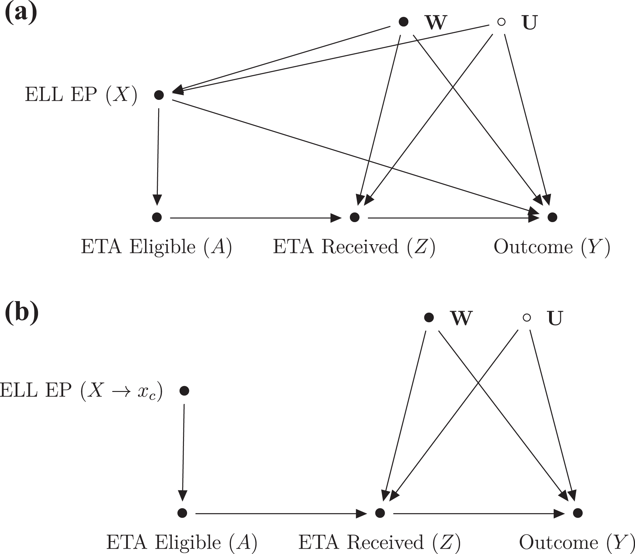
Causal directed acyclic graph (DAG) and causal graphical identification for evaluating the effects of ETA. ETA Eligible (A) represents students’ ETA eligibility status. ELL EP (X) represents ELL English proficiency. ETA Received (Z) represents whether students received ETA or not, and Outcome represents students’ math-proficiency outcome. $W$ represents measured covariates, and $U$ represents unmeasured covariates. (a) Causal DAG. (b) Causal graphical identification. Note. ETA = extended time accommodation; ELL = English-language learner.

Although the graph suggests that conditioning on ELL English proficiency (X) blocks the confounding backdoor paths between ELL eligibility (A) and students’ outcome (Y),¹ the causal effect of A on Y is nonetheless not identified because the positivity assumption is not met. That is, for each value of the running variable X, we only observe either eligible or ineligible students, but never both (i.e., there is complete lack of overlap). The causal effect of ETA receipt (Z) on the outcome (Y) would be identified conditional on $W$ and $U$ , but only if (i) all variables in $U$ were observed and (ii) positivity held, that is, within each value of $W$ and $U$ , the probability of receiving treatment is strictly between zero and one. But given the lack of overlap and the presence of unobserved $U$ , we exploit the discontinuity at the cutoff rather than matching methods to identify the causal effect of ETA on the math-proficiency outcome.

Figure 1(b) shows the causal graph for the RD design at the limiting cutoff score, $X \to x_{c}$ (Steiner et al., 2017). In the limit, the running variable (X) still determines ETA eligibility (A) but neither directly affects the outcome (Y) nor is determined by variables $W$ and $U$ . Thus, in the close vicinity of the cutoff score, ETA eligibility is independent of $W$ and $U$ (local randomization), and thus, the ITT at the cutoff (i.e., the effect transmitted along $A \to Z \to Y$ ) is identified without any covariate adjustments for $W$ and $U$ . Using A as an instrument for ETA receipt (Z) identifies the $τ_{LATE} (x_{c})$ at the cutoff (i.e., the effect $Z \to Y$ ).

3. RD Design With an Ordinal Running Variable

So far, we have assumed that the running variable X is continuous. However, in practice, many RD designs rely on a discrete metric running variable, such that the causal effects at the limiting cutoff are no longer nonparametrically identified. The identification of causal effects then requires parametric functional form assumptions to bridge the gap between the neighboring discrete values at the cutoff (Lee & Card, 2008). With ordinal running variables, as for our ETA study, causal identification is even more challenging because the ordinal categories first need to be mapped onto an appropriate numerical scale. In this section, we discuss the identification and estimation of causal effects from RD designs with an ordinal running variable. Drawing valid and reliable causal conclusions from such RD designs requires three main steps. First, researchers need to decide on a reasonable scaling function for the ordinal running variable. Second, they need to correctly specify the outcome regression with respect to the chosen scaling function and estimate standard errors that reflect specification errors due to the running variable’s discreteness. Third, given uncertainties about the appropriate scaling and correct model specification, researchers should always conduct a set of sensitivity analyses to probe the conclusions’ robustness to (i) the choice of the scaling function, (ii) the choice of the scaled cutoff score, and (iii) remaining confounding due to model misspecification. The following subsections describe these steps in detail and state the causal identifying assumptions.

3.1. Scaling Function

The scaling function $S (ω_{k})$ maps the K categories $ω_{1}, \dots, ω_{K} \in Ω$ of the ordinal running variable onto the real numbers $ℝ$ ; in classical measurement and test theory, $S (ω_{k})$ is often referred to as a scaling rule. Each category $ω_{1} {,…,ω}_{K}$ is assigned to a numerical score $S (ω_{k}) = x_{k}$ $(k = 1, \dots, K)$ , and we refer to $x_{1}, \dots, x_{K}$ as scale values. Importantly, the scaling function S preserves the rank order from the ordinal running variable (Crocker & Algina, 2006).

There are a variety of scaling functions that map ordinal categories onto real numbers. First, ordinal categories can be arranged in ascending order, and their ranks are used as scale values (Crocker & Algina, 2006). For instance, in our ETA study, ELL English proficiency has six categories ranging from No Proficiency to Never ELL. Thus, No Proficiency translates into a scale value of $S (ω_{1}) = 1$ , ELL Beginning into $S (ω_{2}) = 2$ , and Never ELL into $S (ω_{6}) = 6$ . The rank-based scaling function presumes that there are equal distances between adjacent categorical levels, and the scale values have a meaningful metric interpretation.

However, rank-based scale values might be a poor choice when equal distances between consecutive categories are not a suitable representation of the ordinal levels in the running variable. In this case, researchers should consider optimal scaling techniques that use observed variables directly related to the categories of the ordinal running variable (Bradley et al., 1962). Such a variable could be the underlying continuous variable that measures the same proficiency/skill or a close proxy thereof (e.g., a continuous composite English-proficiency score, domain scores like reading and writing, or English-proficiency scores from previous grades). Then, the optimal scale values can be determined using optimal scaling methods for categorical data like categorical regression or categorical principal components analysis. Here, optimality is often defined by maximization of variance, maximization of pairwise linear relationships, or maximization of homogeneity among variables, to name a few. Also, if multiple categories receive similar scale values, we can collapse these categories into one category (Bradley et al., 1962; Machines, 2019; Meulman, 1998; Meulman et al., 2019).

In the absence of related continuous variables that could be used for optimal scaling techniques, it is sometimes possible to infer scale values from external sources like published cut scores used to form the categories. Specifically, if there were clearly defined cut scores on the ELL English-proficiency variable, then the midpoints of the cut scores could be used as scale values. However, the midpoints of the lowest and highest category might not be meaningfully defined if the minimum or maximum of the ELL proficiency score is not known or is a very extreme value that is rarely observed. If cut scores for the ordinal running variable are not known, we can use other related classifications based on the same or similar underlying continuous variable. For example, the Wisconsin Department of Instruction defines English-language-proficiency classifications with seven ordinal levels (ELL Beginning Preproduction, ELL Beginning Production, ELL Intermediate, ELL Advanced Intermediate, ELL Advanced, Formerly ELL, and Never ELL) that are very similar to the observed ordinal categories of English proficiency in NAEP. After mapping the different ordinal categories, we could use their cut scores and corresponding midpoints to obtain scale values.

3.2. Sharp RD Designs With an Ordinal Running Variable

As mentioned before, with an ordinal running variable, nonparametric causal identification breaks down because in the close vicinity of the cutoff score (i.e., the ELL Advanced category) only students eligible for ETA are observed and there are no ineligible control students. Given the identification failure at the limiting cutoff, the limiting graph in Figure 1(b) no longer applies either. Thus, we are back to the graph in Figure 1(a), which indicates that the observed and unobserved sets of covariates $W$ and $U$ confound the causal relations of interest. But the confounding bias could be removed if the functional relation between the ordinal running variable X and the outcome Y is correctly specified, such that a valid extrapolation of the average control outcome from the ETA ineligible to the eligible students at the ELL Advanced cutoff category becomes possible.

To this end, we extend the approach suggested by Lee and Card (2008) for discrete running variables to ordinal running variables. Instead of the local continuity assumption (A1), we now assume a correctly specified outcome regression, such that the expected control outcome can be correctly inferred by extrapolating the outcome regression for control units to the cutoff category.

(A4) Outcome Regression Function:

$E [Y_{i j} | X_{i j} = x_{k}] = A_{i j} τ (x_{c}) + h_{S} (x_{k})$ with $h_{S} (x_{c}) = E [Y_{i j} (0) | X_{i j} = x_{c}]$ .

Here, $h_{S} (x_{k})$ is a continuous parametric function with respect to the chosen scaling function $S (ω_{k}) = x_{k}$ . The requirement $h_{S} (x_{c}) = E [Y_{i j} (0) | X_{i j} = x_{c}]$ guarantees that the expected potential control outcome at the cutoff score is correctly predicted by $h_{S} (x_{c})$ . The parameter $τ (x_{c})$ is the ATE at the cutoff x_c . Due to the discreteness of $X_{i j}$ , $h_{S} (\cdot)$ must be parametrized by less than K parameters; if $h_{S} (\cdot)$ uses K or more parameters, $τ (x_{c})$ is not identifiable because of multicollinearity.

In estimating and conducting inference for $τ (x_{c})$ , we follow Lee and Card (2008) and add a random specification error with a common variance component for all the observations at any given values of the discrete running variable. This specification error reflects the potential deviation between the expected value of the true outcome at the cutoff and the predicted value based on h_S . The specification error can also be reinterpreted as adding a random effects term in a mixed effects model and, hence, makes it easy to implement in practice (see Section 4.3).

3.3. Fuzzy RD Designs With an Ordinal Running Variable

For fuzzy RD designs with an ordinal running variable, the ITT at the cutoff category is identified and estimated just like the ATE in the sharp RD design, where the treatment assignment status $A_{i j}$ is used as a treatment indicator. Also, the LATE is identifiable and estimable at the cutoff if a functional form assumption analogous to (A4) is met for the expectation of $Z_{i j}$ .

(A5) Treatment Regression Function:

$E [Z_{i j} | X_{i j} = x_{k}] = A_{i j} α + g_{S} (x_{k})$ with $g_{S} (x_{c}) = E [Z_{i j} (0) | X_{i j} = x_{c}]$ .

As before, $g_{S} (x_{k})$ is a continuous parametric function with respect to the scaling function $S (ω_{k}) = x_{k}$ . The term $α$ represents the discontinuity in treatment probabilities at the cutoff and is used to obtain the LATE at the cutoff by taking the ratio between the ITT and $α$ . For Assumption (A4), like before, identifiability demands less than K parameters for $g_{S} (\cdot)$ . Also, in estimating standard errors for the LATE, we take random specification errors in the treatment regression function into account (see Section 4.3 and Supplemental Appendix B in Lee and Card [2008] for details).

3.4. Sensitivity Analyses

The discussions of the assumptions for the sharp and fuzzy RD design revealed that the causal effects at the cutoff are identified only if the scaling function and outcome (and treatment) regressions are correctly specified. Given that the correct specification of the functions is uncertain in practice, researchers should always conduct sensitivity analyses to check the conclusions’ robustness to (i) the choice of scaling functions, (ii) the choice of cutoff values, and (iii) the presence of remaining confounding resulting from a misspecified outcome or treatment regression (that leads to biased extrapolations of the control or treatment outcomes to the cutoff value).

First, in choosing different scaling functions $S (ω_{k}) = x_{k}$ $(k = 1, \dots, K)$ for the ordinal running variable, researchers can probe the robustness of effect estimates (ATE, ITT, and LATE at the cutoff) to alternative plausible choices of $S (ω_{k})$ . Specifically, we use two complementary strategies of determining the scaling functions. The first strategy is to change the distance between the two neighboring categories at the cutoff, $| x_{c} - x_{c + 1} |$ , where $x_{c + 1}$ is the neighboring category belonging to the other treatment condition, while keeping the other distances of neighboring categories unchanged. In this article, the distance $| x_{c} - x_{c + 1} |$ is referred to as a “gap.” Changing the gap as a sensitivity analysis is of particular use when the distance of neighboring categories cannot directly be derived from internal or external information and the choice of the gap is partly deliberate. This affects the distance of extrapolation from the cutoff category (x_c ) to the neighboring category ( $x_{c + 1}$ ), thus potentially producing a different effect estimate. The second strategy is to determine alternative scale values for all K categories ( $ω_{1}, \dots, ω_{c}, \dots, ω_{K}$ ); that is, the distances between all neighboring categories may be changed simultaneously. As mentioned before, the scaling function for the ordinal running variable can be determined by relevant external criteria or by optimal scaling methods with respect to the underlying continuous variable or a proxy measure thereof. If the effect estimates are robust to the choice of alternative scaling functions, researchers can be more confident in their conclusions about the presence or absence of a treatment effect.

Second, given a particular scaling function, one may evaluate the effect estimates at different cutoff value x_c between the scale value of the cutoff category $S (ω_{c})$ and the value of the neighboring category $S (ω_{c + 1})$ . Such a sensitivity analysis reflects the uncertainty about the cutoff point’s location due to the use of the ordinal running variable and provides further evidence for the robustness of the effect estimates. This type of sensitivity analysis is particularly needed if there is ambiguity about where the cutoff value of interest should be placed on the metric scale. However, a different cutoff point changes the underlying local target population because the RD design identifies the ATE for the population at the cutoff point only. Thus, variations in effect estimates from the sensitivity analysis might be due to differences in the local populations as well as potentially misspecified functional forms. But, because our sensitivity analysis only varies the cutoff between two neighboring ordinal cutoff categories (e.g., from x_c to $1 / 2 \cdot | x_{c} + x_{c + 1} |$ ), we suspect that the local populations are similar and the corresponding variations in the effect estimates will be negligibly small. Thus, in this article, estimating LATEs between the two cutoff categories is used only for the purpose of sensitivity analysis, with less concern for defining and interpreting the underlying local populations.

Finally, it is advisable to probe whether the conclusions drawn are sensitive to unblocked confounding due to model misspecification of h_S (and g_S for the LATE). The effect estimates at the cutoff are unbiased only if the extrapolations are based on a correctly specified functional form h_S (and g_S ) with respect to the chosen scaling function S. With a misspecified functional form, the extrapolation to the cutoff score may become invalid and fail to completely remove confounding bias between the outcomes of treatment subjects in the cutoff category and the outcomes of control subjects in the neighboring category. For example, suppose that we simply compare the mean outcomes of the neighboring categories Advanced ELL (treated subjects) and Formerly ELL (control subjects) in our empirical example. That is, we make no attempt to remove any confounding between the treatment and control groups. Thus, the resulting unadjusted effect estimate likely suffers from confounding bias due to group differences in ELL English-proficiency categories and in any other student characteristics like ability or the number of English-language books read per month. The RD design with an ordinal running variable tries to overcome differences between the neighboring treatment and control groups by adjusting for covariates through a correct specification of h_S (and g_S ). Since misspecified functional forms may remove a part but not all the confounding bias, researchers should conduct sensitivity analyses and evaluate the degree of effect variations obtained from the sensitivity analysis. We demonstrate all these sensitivity analyses with our empirical example in the next section.

4. Empirical Example: Testing Accommodations in NAEP

4.1. Data and Variables

NAEP is the largest nationally representative and continuing assessment of what students in the United States know and can do in various disciplines. The data have been collected by NCES within the Institute of Education Sciences. The 2017 NAEP assessments were conducted for Grades 4 and 8 in mathematics, reading, and writing. The NAEP sampling procedures ensure that the students and schools selected in NAEP are representative of the target population. The NAEP assessment strives to minimize participant burden by giving students a subset of items from the total item pool (Johnson, 1992; Oranje & Kolstad, 2019). For more details of the NAEP methods and procedures, see the NAEP page of the NCES website (https://nces.ed.gov/nationsreportcard/tdw/).

In our study, we used the NAEP Grade-4 2017 restricted-use data for mathematics. For the data analysis, we excluded (i) schools with only one student, (ii) SDs, and (iii) ELL students whose prior performance was below the grade level of performance of NAEP; here, ELL students’ prior performance was evaluated by their teachers or school staff members through an ELL questionnaire. After sample exclusion, our final analysis sample consisted of 116,910 students from 7,450 schools (78.2% of the original reporting sample).²

In the 2017 NAEP data, we used the math proficiency as the outcome $Y_{i j}$ . As mentioned earlier, ETA eligibility $A_{i j}$ is binary with $A_{i j} = 1$ denoting that a student is eligible for ETA and $A_{i j} = 0$ denoting that a student is ineligible for ETA. The eligibility status is determined by ELL English proficiency, derived from students’ prior ELL status and ELL English proficiency in reading. Specifically, ELL English proficiency was reported with six ordinal levels: No Proficiency, ELL Beginning, ELL Intermediate, ELL Advanced, Formerly ELL, and Never ELL; see survey questionnaires from the NAEP website (https://nces.ed.gov/nationsreportcard/experience/survey_questionnaires.aspx). However, in following school-specific rules and resources, school staff decided which students actually received ETA. The data indicate two-sided noncompliance; some students eligible for ETA did not receive ETA ( $A_{i j} = 1$ but $Z_{i j} = 0$ ), while some ineligible students received ETA ( $A_{i j} = 0$ but $Z_{i j} = 1$ ). For the outcome and treatment regressions, we used a set of pretreatment covariates $W_{i j}$ , including gender, race/ethnicity, free lunch status, English instruction period, U.S. school period, and primary language; these variables partially explain why some eligible students did not receive ETA. For a full list of pretreatment covariates and their distributions, see Supplemental Appendix A.

In demonstrating our proposed approach, we only used the last of the 20 plausible values in math proficiency as the outcome $Y_{i j}$ (mean = 244.05, SD = 28.25) and do not incorporate multiple plausible values. We also ignore sampling weights and the corresponding jackknife replicate weights provided by the 2017 NAEP data. This allows us to discuss the analyses without getting distracted by the more complex measurement and sampling design. But to generalize our findings, we briefly explain in Supplemental Appendix C how to analyze NAEP data with multiple plausible values and sampling weights and provide results via the EdSurvey R package (Bailey et al., 2020; R Core Team, 2020).

4.2. Choice of Scaling Function and Cutoff Score

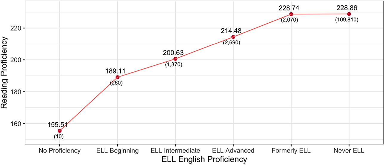
To assess the effects of ETA with an RD design, we first chose the scaling function for the ordinal ELL English categories based on their ranks, $S (ω_{k}) = k$ , assuming that the performance differences between consecutive categories are approximately equidistant. The equidistance assumption might be justified because we found that the differences in the reading proficiency scores across consecutive categories were similar except for the two extreme levels (No Proficiency and Never ELL) from the 2017 NAEP data (see Figure 2).³ Thus, we assigned 1 to No Proficiency, 2 to ELL Beginning, 3 to ELL Intermediate, 4 to ELL Advanced, 5 to Formerly ELL, and 6 to Never ELL. The cutoff score is $x_{c} = 4$ , which corresponds to the ELL Advanced category.

Figure 2.

Observed means in reading by English-language learner English proficiency. Note. Numbers in parentheses represent sample sizes and are rounded to nearest tens. Source. U.S. Department of Education, National Center for Education Statistics, National Assessment of Educational Progress (NAEP) 2017.

4.3. Parametric Model Specifications

Given two-sided noncompliance, we estimate the ITT and the LATE at the cutoff. Following Lee and Card (2008), we model the categories of the ordinal running variable as random effects in a hierarchical linear model that also accounts for the clustered data structure of students nested within schools. The reading proficiency $Y_{i j k}$ for a student i, school j, and ELL category k is modeled as follows:

Y_{i j k} = β_{0} + β_{1} A_{i j k} + β_{2} (X_{i j k} - x_{c}) + β_{3} A_{i j k} (X_{i j k} - x_{c}) + \sum β_{w} W_{i j k} + s_{j} + u_{k} + ε_{i j k},

A_{i j k} = {\begin{matrix} 1, & X_{i j k} \leq x_{c} \\ 0, & X_{i j k} > x_{c}, \end{matrix} x_{c} = 4.

In the model equation, the ITT at the cutoff is given by $β_{1} = τ (x_{c})$ , where the cutoff is set to the ELL Advanced category, that is, the average effect of ETA eligibility for the students with ELL Advanced. The term $β_{0}$ represents the estimated average control outcome at the cutoff. The term $β_{2}$ represents the slope coefficient for scale values above the cutoff value, and the term $β_{3}$ represents the slope difference between scale values below the cutoff value and those above the cutoff value. Due to the limited number of ELL categories, we did not consider a polynomial term of the running variable that could lead to overfitting. The model also includes a set of measured pre-treatment covariates (potential confounders) $W_{i j}$ , the school random effects term s_j , and the random specification error u_k . To probe whether the proposed model is correctly specified, we used a residual analysis and compared predicted outcome means of the running variable from the estimated model to the corresponding observed means (see Figure 3).

Figure 3.

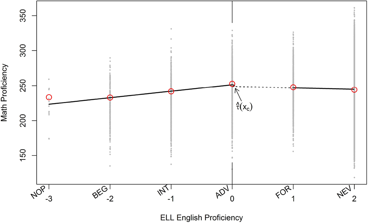
Regression discontinuity design for evaluating the effects of extended time accommodations in mathematics. Note. NOP = No Proficiency; BEG = ELL Beginning; INT = ELL Intermediate; ADV = ELL Advanced; FOR = Formerly ELL; NEV = Never ELL. The solid black lines represent the estimated regression function, and the dotted gray line represents the extrapolated line from the regression function. Gray points indicate students’ math scores, and open red points indicate covariate-adjusted observed outcome means with cell means coding. Source. U.S. Department of Education, National Center for Education Statistics, National Assessment of Educational Progress (NAEP) 2017.

For estimating the LATE effect at the cutoff, we use an instrumental variable regression or two-stage least squares (TSLS) regression. That is, we treat the model for $Z_{i j k}$ as the first-stage regression and the model for $Y_{i j k}$ as the second-stage regression, and we utilize a TSLS procedure with random effect terms to estimate the LATE. Specifically, the TSLS models for $Z_{i j k}$ and $Y_{i j k}$ are as follows:

Z_{i j k} = α_{0} + α_{1} A_{i j k} + α_{2} (X_{i j k} - x_{c}) + α_{3} A_{i j k} (X_{i j k} - x_{c}) + \sum α_{w} W_{i j k} + s_{j} + u_{k} + ε_{i j k},

Y_{i j k} = γ_{0} + γ_{1} {\hat{Z}}_{i j k} + γ_{2} (X_{i j k} - x_{c}) + γ_{3} A_{i j k} (X_{i j k} - x_{c}) + \sum γ_{w} W_{i j k} + s_{j} + u_{k} + ε_{i j k} .

In the first-stage regression (2), $α_{1}$ is the discontinuity in the treatment receipt probabilities between eligible students and noneligible students at the cutoff, and $α_{0}$ is the estimated average probability of receiving ETA for noneligible students at the cutoff. $α_{2}$ is the slope coefficient for scale values above the cutoff value, and $α_{3}$ is the slope difference between scale values below the cutoff value and those above the cutoff value. We also add measured covariates $W_{i j}$ , the school random effect term s_j , and the random specification error u_k . In the second-stage regression (3), the predicted values ${\hat{Z}}_{i j k}$ are used as a regressor instead of $A_{i j k}$ . Then, we can estimate $γ_{1} = τ_{LATE} (x_{c})$ that represents the LATE at the cutoff of ELL Advanced, that is, the effect of receiving ETA among the complier students in the ELL Advanced category. Standard errors in all models were estimated using cluster bootstrap sampling with 2,000 replicates,⁴ and all models were estimated using the lme4 R package (Bates et al., 2015).

4.4. Results

Table 1 summarizes the students’ ETA eligibility, as defined by ELL status, and whether they actually received the ETA. Overall, about 4.2% of the students (4,940 students) in our study sample were eligible for ETA; these are denoted as ELL students in the table. Among those who were eligible for ETA, about 32.5% of the ETA-eligible students (i.e., ELL) actually received ETA. Also, we saw that few students received ETA even though they were not eligible for ETA (i.e., non-ELL), likely due to test irregularities; see more details on the compliance rate by ELL English-proficiency categories in Supplemental Appendix B.

Table 1.

Compliance for Extended Time Accommodations (ETAs) by English-Language Learner (ELL) Status

Eligibility	ETA
Eligibility	Nonreceived	Received	Total
Non-ELL	111,940	30	111,970
ELL	3,340	1,610	4,940
Total	115,270	1,640	116,910

Note. Numbers are rounded to nearest tens. Details may not sum to a total due to rounding.

Source. U.S. Department of Education, National Center for Education Statistics, National Assessment of Educational Progress (NAEP) 2017.

Figure 3 provides a visual representation of the RD design, where the x-axis represents the rank-based scale values of English-proficiency categories with the cutoff point defined at ELL Advanced and the y-axis represents the math proficiency scores. For each ELL category, covariate-adjusted observed outcome means (with cell means coding) are shown by red circles. Since the observed and predicted means (from the fitted model) are very similar, except for the No Proficiency category with relatively few observations, the linear model provides good fit to the data near the cutoff. We observe that the mean math-proficiency score of Never ELL was similar to that of Formerly ELL, and the mean math-proficiency score increased when ELL English proficiency increased from No Proficiency to ELL Advanced. We can also visually see that the ITT effect at the cutoff is small.

Table 2 summarizes ITT and LATE estimates. We interpret 95% confidence intervals as “compatibility intervals” (Amrhein et al., 2019), that is, the set of possible true effects that are compatible with our data for the given model. As seen from Table 2, the ITT estimate is 2.66 points and small. Also, under the above assumptions, our data are compatible with ITT effects as small as −4.36 points and as large as 6.12 points. The interval suggests that the ITT could be (close to) zero or positive and we do not have sufficient power to reject the null hypothesis of no effect. In contrast, the LATE estimate is larger than the ITT estimate, and all values in the interval are positive; the LATE estimate is 12.99 points, and the interval indicates compatibility with effects between 7.25 and 19.53 points.

Table 2.

Intent-to-Treatment (ITT) Effect and Local Average Treatment Effect (LATE) Estimates of Extended Time Accommodations at the Cutoff

Estimand	Estimate	Standard Error	95% Confidence Intervals
ITT	2.66	2.67	[−4.36, 6.12]
LATE	12.99	3.14	[7.25, 19.53]

Source. U.S. Department of Education, National Center for Education Statistics, National Assessment of Educational Progress (NAEP) 2017.

Finally, we remark that given that we have only two categories to the left of the cutoff category, the extrapolation of the control outcomes from the Formerly ELL category to the Advanced ELL category strongly depends on the mean math proficiency of the Never ELL category. If students with Never ELL would on average score slightly higher or lower, the effect estimates at the cutoff could change their sign. Thus, the student composition of the Never ELL category is potentially influential on the ETA evaluation. In NAEP, the Never ELL category includes students who (1) are native English speakers, (2) have never been designated as ELL, or (3) were designated as ELL students more than 2 years ago. The inclusion of native English speakers in the Never ELL category is problematic because they do not belong to our target population of interest (i.e., nonnative speakers). Unfortunately, the NAEP data do not provide individual-level information about whether a student belongs to one of the three subcategories. To address potential bias concerns, we did a subgroup analysis only with Hispanic students because a smaller portion of them are native English speakers (de Brey et al., 2019). We found that the ITT effect may be slightly smaller than the ITT with the original sample, while the LATE does not differ much (see results in Supplemental Appendix D).

4.5. Sensitivity Analyses

4.5.1. Methods

We assess the sensitivity of our conclusions against (i) the choice of the scaling function, (ii) the choice of the cutoff value, and (iii) remaining confounding. To probe the results’ sensitivity to different choices of the scaling function, we first decreased or increased the gap between the two neighboring cutoff categories (i.e., ELL Advanced and Formerly ELL) on our original scale. It assesses the effect estimates’ sensitivity to uncertainties in the appropriate scaling between the two neighboring categories at the cutoff. A larger gap increases reliance on extrapolation than a smaller gap, and thus, the former might be more susceptible to model misspecification. We consider two cases, one with a reduced gap and the other with an increased gap. For the reduced gap, we used scale values (−3, −2, −1, 0, 0.5, and 1.5), and for the increased gap, we used (−3, −2, −1, 0, 1.5, and 2.5). All of the scale values were centered at the cutoff of ELL Advanced.

Next, we used a different set of scale values for all categories (and not only the neighboring cutoff categories) based on the cut scores of the proficiency categories from the ACCESS for ELLs exam in World-Class Instructional Design and Assessment (WIDA).⁵ WIDA’s (2013, 2019) English-proficiency levels consist of Entering, Emerging, Developing, Expanding, Bridging, and Reaching for ELL students and former ELL students. From the description of WIDA’s proficiency levels, we considered Entering, Emerging, Developing, Bridging, and Reaching as being aligned with No proficiency, ELL Beginning, ELL Intermediate, ELL Advanced, and Formerly ELL, respectively, and we used the cut scores from reading proficiency levels of fourth graders (WIDA, 2013) to determine the scale values. Specifically, based on the cut scores of the WIDA’s proficiency levels, we computed the mean scores (i.e., midpoints) of the first four proficiency levels and used the relative differences between consecutive proficiency levels as scale values. For noneligible students, we assigned the same scale value to the last two categories because Formerly ELL and Never ELL’s reading performance was similar from Figure 2. Ultimately, we used the scale values of (−5.6, −2.2, −1, 0, 1, and 1) for our sensitivity analysis, with 0 indicating ELL Advanced.

We also conducted a sensitivity analysis with respect to the choice of the cutoff point. Specifically, we varied the cutoff value by redefining the cutoff value as the mean between the scale values of ELL Advanced and Formerly ELL; we call the new cutoff point “Between.”

Lastly, for the sensitivity analysis against remaining confounding, we used the general bias formula from VanderWeele and Arah (2011), where the potential bias d arising from unmeasured confounders can be represented by the product $δγ$ . $δ$ characterizes a constant prevalence difference of a binary hypothetical confounder between the treatment groups and $γ$ characterizes a constant outcome difference between the levels of the hypothetical confounder.

4.5.2. Results

Figure 4 visualizes the sensitivity analysis for ITT estimates by changing the choice of the scaling functions and the choice of the cutoff values. Figure 5 displays the corresponding point estimates and confidence intervals.

Figure 4.

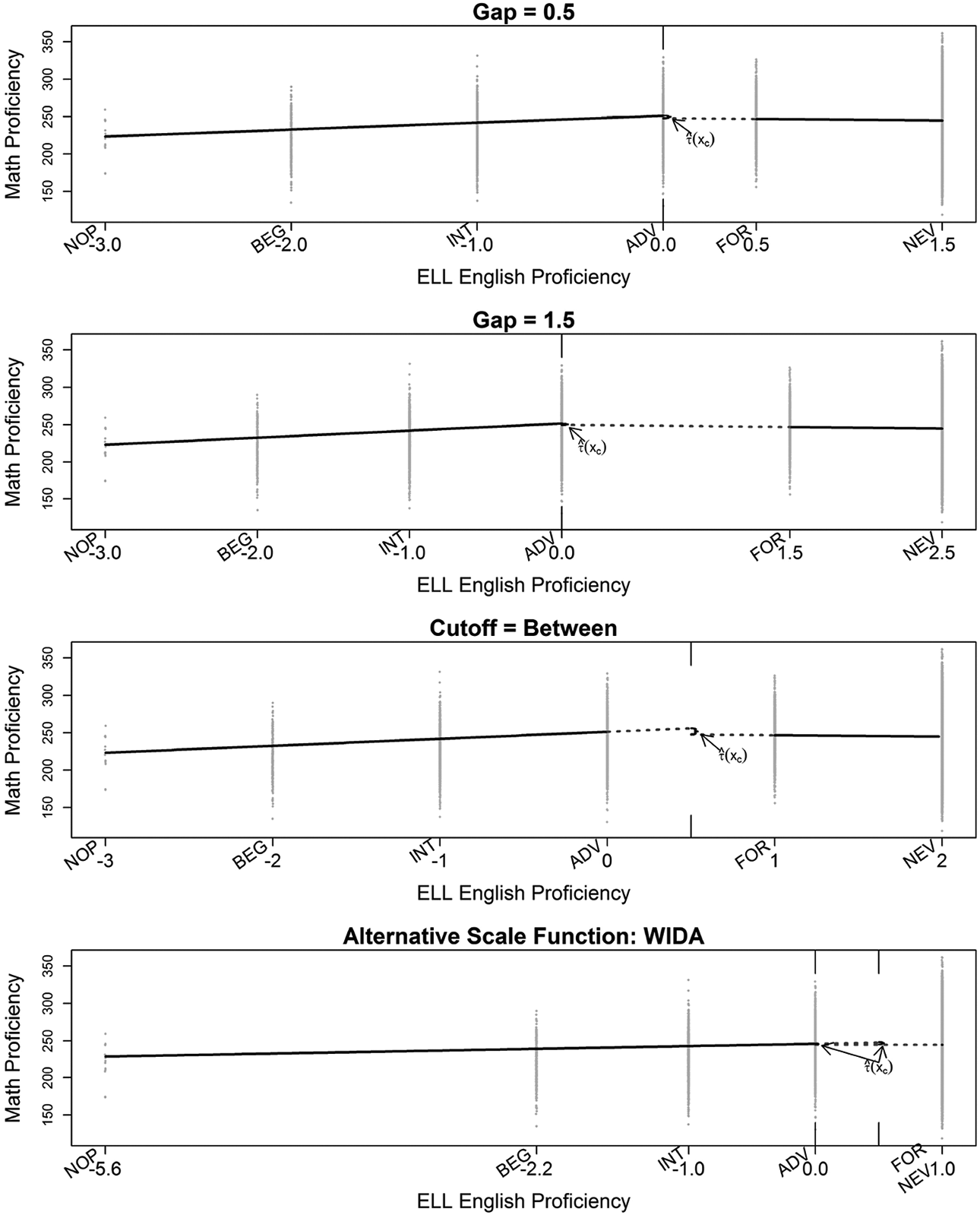
Sensitivity analysis against scaling. Note. NOP = No Proficiency; BEG = ELL Beginning; INT = ELL Intermediate; ADV = ELL Advanced; FOR = Formerly ELL; NEV = Never ELL. The solid black lines represent the estimated regression function, and the dotted gray lines represent the extrapolated line from the regression function. Gray points indicate students’ math scores. Source. U.S. Department of Education, National Center for Education Statistics, National Assessment of Educational Progress (NAEP) 2017.

Figure 5.

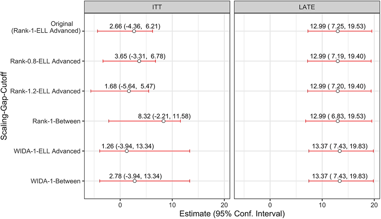
Estimates and confidence intervals of the intent-to-treatment effect and local average treatment effect from sensitivity analysis against scaling. Source. U.S. Department of Education, National Center for Education Statistics, National Assessment of Educational Progress (NAEP) 2017.

From Figures 4 and 5, we observed that all the ITTs are compatible with no effect although the confidence intervals of the ITT vary depending on the combinations of scaling, gap, and cutoff points. In contrast, the LATEs remain positive and the confidence intervals of the LATE are very similar across different choices of the scaling function.⁶ Overall, our original conclusions about the ITT and LATE are robust to different specifications of the scaling function and the cutoff value.

Next, we tested the sensitivity of our results to remaining confounding and evaluated the degree of effect variations introduced by negative and positive unmeasured confounding bias. Specifically, we estimated a new adjusted treatment effects $τ^{†}$ for the ITT and LATE based on the formula from VanderWeele and Arah (2011): $d = δγ = τ - τ^{†}$ by considering the causal graph in Figure 1(a), where $U$ is a set of unobserved confounders. Here, we use a single independent and binary confounder U to represent the $U$ -induced confounding bias after conditioning on the observed covariates $W$ . Then, $δ$ represents the magnitude of the causally reverse effect of A on U (i.e., $A \to U$ ), and $γ$ represents the causal effect of the confounder U on Y ( $U \to Y$ ). Thus, the bias induced by this hypothetical confounder is $d = δγ$ . Also, the bias-adjusted effect is $τ^{†} = τ - d = τ - δγ$ . To implement the sensitivity analysis, we first need to find reasonable values for $δ$ and $γ$ . We determined $δ$ by looking at the absolute mean differences in the measured covariates $W$ between the neighboring ELL Advanced and Formerly ELL groups. The largest difference we observed is $δ = 0.07$ (see Table E1 of Supplemental Appendix E in choosing the value of $δ$ ). For $γ$ , we use the absolute value of the largest estimated coefficient of the measured covariates in the outcome model (see Supplemental Appendix E) and set $γ = 17.16$ .

For the ITT estimate, we use a negative bias of $d = - 0.07 \times 17.16 = - 1.20$ and obtain a bias-adjusted effect $τ_{1}^{†} = 2.66 + 1.20 = 3.86$ with its corresponding 95% confidence interval [−3.16, 7.32]. For the corresponding positive bias, we obtain a new adjusted effect of $τ_{2}^{†} = 2.66 - 1.20 = 1.46$ and its confidence interval of [−5.56, 4.92]. Regardless of the direction of bias, the new adjusted effects are compatible with no effect and the new confidence intervals substantially overlap with the original confidence interval in Table 2. Thus, the conclusion about ITT does not change in the presence of unmeasured confounding (at least with regard to the magnitude of observed confounding effects). For the LATE estimate, we use a negative bias of −1.20 and obtain a bias-adjusted effect of $τ_{1}^{†} = 12.99 + 1.20 = 14.19$ and an adjusted 95% confidence interval of [8.45, 20.73]. For the corresponding positive bias, we obtain a new adjusted effect of $τ_{2}^{†} = 12.99 - 1.20$ $= 11.79$ with the confidence interval of [6.05, 18.33]. The new adjusted effects are compatible with positive effects that are clearly greater than zero, and the adjusted confidence intervals strongly overlap with the original confidence interval in Table 2. Thus, we conclude that the LATE estimate is quite robust to unmeasured confounding.

5. Conclusions

In this article, we proposed to use an RD design with an ordinal discrete running variable. We used a scale function S to convert the ordinal levels of the running variable to numeric scale values and modified Lee and Card’s (2008) framework to accommodate the ordinal running variable. We assessed the sensitivity of our results with respect to the choice of the scaling function and the cutoff value. We also assessed the sensitivity of our results to remaining confounding arising from an incorrect scaling function or an imperfect functional form. We demonstrated the proposed approach by investigating the effects of ETA on students’ math performance based on the 2017 NAEP data. Overall, we found that our ITT results of being eligible for ETA at the cutoff are compatible with slightly negative but also positive effects, whereas our LATE results of receiving ETA indicate positive effects. Our sensitivity analyses indicate that our original ITT and LATE are robust to various design-based factors for sensitivity analyses (i.e., the choice of the scaling function, the choice of the cutoff value, and remaining confounding).

Based on our findings, we provide some suggestions for future research concerning evaluation of testing accommodations based on an RD framework. First, Kolesár and Rothe (2018) showed that Lee and Card’s (2008) confidence intervals with standard errors that are clustered by a discrete running variable underestimate coverage properties. Future research would use alternative confidence intervals which guarantee accurate coverage properties, proposed by Kolesár and Rothe (2018). Second, if the NAEP assessment provides continuous ELL English proficiency that was used to determine ETA eligibility, it will enable researchers to estimate the ITT and LATE at the cutoff with less concerns about biases arising from the choice of the scaling function or the functional form of the outcome model. Third, if an ordinal running variable is present and a relevant underlying variable, such as pretest English scores in our setting, is included in the observed data, researchers could use optimal scaling techniques to choose appropriate scale values. Lastly, we did not consider whether students made use of ETA in our study. That is, even if the student received ETA, students may have not needed the extra allotted time. Based on prior works on accommodations, about 40% of the students who received ETA made use of the extra time in the NAEP assessment (Kim & Circi, 2018, 2019). Students’ actual use of ETA can be determined by process data, which are data provided by examinees’ responses to the testing devices while taking the test (Bergner & von Davier, 2018). If such data are available, we may have to use sequential compliance models and it would be interesting to incorporate them into RD designs in order to assess the effect of making use of ETA.

Supplemental Material

Supplemental Material, sj-pdf-1-jeb-10.3102_10769986221090275 - Regression Discontinuity Designs With an Ordinal Running Variable: Evaluating the Effects of Extended Time Accommodations for English-Language Learners

Supplemental Material, sj-pdf-1-jeb-10.3102_10769986221090275 for Regression Discontinuity Designs With an Ordinal Running Variable: Evaluating the Effects of Extended Time Accommodations for English-Language Learners by Youmi Suk, Peter M. Steiner, Jee-Seon Kim and Hyunseung Kang in Journal of Educational and Behavioral Statistics

Footnotes

Declaration of Conflicting Interests

The author(s) declared no potential conflicts of interest with respect to the research, authorship, and/or publication of this article.

Funding

The author(s) disclosed receipt of the following financial support for the research, authorship, and/or publication of this article: This work was supported by a grant from the American Educational Research Association Division D.

Notes

References

Amrhein

Greenland

MsShane

(2019). Retire statistical significance. Nature, 567, 305–307. https://doi.org/10.1038/d41586-019-00857-9

Bailey

Emad

Huo

Lee

Liao

Lishinski

Nguyen

Xie

Zhang

Buehle

C’deBaca

(2020). EdSurvey: Analysis of NCES education survey and assessment data [Computer software manual]. Retrieved from https://CRAN.R-project.org/package=EdSurvey (R package version 2.5.0)

Bates

Mächler

Bolker

Walker

(2015). Fitting linear mixed-effects models using lme4. Journal of Statistical Software, 67(1), 1–48. https://doi.org/10.18637/jss.v067.i01

Bergner

von Davier

A. A.

(2018). Process data in NAEP: Past, present, and future. Journal of Educational and Behavioral Statistics, 44(6), 706–732. https://doi.org/10.3102/1076998618784700

Bradley

Katti

Coons

I. J.

(1962). Optimal scaling for ordered categories. Psychometrika, 27(4), 355–374. https://doi.org/10.1007/BF02289644

Crocker

Algina

(2006). Introduction to classical and modern test theory. Cengage Learning.

de Brey

Musu

McFarland

Wilkinson-Flicker

Diliberti

Zhang

Branstetter

Wang

. (2019). Status and trends in the education of racial and ethnic groups 2018 (NCES 2019-038). National Center for Education Statistics. Retrieved from https://nces.ed.gov/pubs2019/2019038.pdf

Elwert

(2013). Graphical causal models. In Morgan

S. L.

(Ed.), Handbook of causal analysis for social research (pp. 245–273). Springer. https://doi.org/10.1007/978-94-007-6094-3_13

Gregg

Nelson

J. M.

(2012). Meta-analysis on the effectiveness of extra time as a test accommodation for transitioning adolescents with learning disabilities: More questions than answers. Journal of Learning Disabilities, 45(2), 128–138. https://doi.org/10.1177/0022219409355484

10.

Hahn

Todd

van der Klaauw

(2001). Identification and estimation of treatment effects with a regression-discontinuity design. Econometrica, 69(1), 201–209. https://doi.org/10.1111/1468-0262.00183

11.

Hong

Raudenbush

S. W.

(2006). Evaluating kindergarten retention policy: A case study of causal inference for multilevel observational data. Journal of the American Statistical Association, 101(475), 901–910. https://doi.org/10.1198/016214506000000447

12.

Imbens

G. W.

Lemieux

(2008). Regression discontinuity designs: A guide to practice. Journal of Econometrics, 142(2), 615–635. https://doi.org/10.1016/j.jeconom.2007.05.001

13.

Johnson

E. G.

(1992). The design of the National Assessment of Educational Progress. Journal of Educational Measurement, 29(2), 95–110. https://doi.org/10.1111/j.1745-3984.1992.tb00369.x

14.

Jonson

J. L.

Trantham

Usher-Tate

B. J.

(2019). An evaluative framework for reviewing fairness standards and practices in educational tests. Educational Measurement: Issues and Practice, 38(3), 6–19. https://doi.org/10.1111/emip.12259

15.

Kim

Y. Y.

Circi

(2018). The extended time accommodation (ETA) and performance of students with ETA. Paper presented at the annual meeting of the National Council on Measurement in Education, New York, USA.

16.

Kim

Y. Y.

Circi

(2019). Effects of the extended time accommodation on performance in NAEP mathematics. Paper presented at the annual meeting of the National Council on Measurement in Education, Toronto, Canada.

17.

Kolesár

Rothe

(2018). Inference in regression discontinuity designs with a discrete running variable. American Economic Review, 108(8), 2277–2304. https://doi.org/10.1257/aer.20160945

18.

Lee

D. S.

Card

(2008). Regression discontinuity inference with specification error. Journal of Econometrics, 142(2), 655–674. https://doi.org/10.1016/j.jeconom.2007.05.003

19.

Lee

D. S.

Lemieux

(2010). Regression discontinuity designs in economics. Journal of Economic Literature, 48(2), 281–355. https://doi.org/10.1257/jel.48.2.281

20.

Mercatanti

Mäkinen

Silvestrini

(2021). A regression discontinuity design for ordinal running variables: Evaluating central bank purchases of corporate bonds. The Annals of Applied Statistics, 15(1), 304–322. https://doi.org/10.1214/20-AOAS1396

21.

Machines

I. B

. (2019). IBM SPSS Categories 26. IBM Corporation. Retrieved from ftp://public.dhe.ibm.com/software/analytics/spss/documentation/statistics/26.0/en/client/Manuals/IBM_SPSS_Categories.pdf

22.

Meulman

J. J.

(1998). Optimal scaling methods for multivariate categorical data analysis. SPSS White Paper.

23.

Meulman

J. J.

van der Kooij

A. J.

Duisters

K. L. W.

(2019). ROS regression: Integrating regularization with optimal scaling regression. Statistical Science, 34(3), 361–390. https://doi.org/10.1214/19-STS697

24.

Morgan

S. L.

Winship

. (2014). Counterfactuals and causal inference: Methods and principles for social research. Cambridge University Press. https://doi.org/10.1017/CBO9781107587991

25.

National Center for Education Statistics. (2017a). 2017 Mathematics grades 4 and 8 assessment report cards: Summary data tables for national and state sample sizes, participation rates, proportions of SD and ELL students identified, and types of accommodations. Retrieved from https://www.nationsreportcard.gov/math_2017/files/2017_Technical_Appendix_Math_State.pdf

26.

National Center for Education Statistics. (2017b). 2017 Reading grades 4 and 8 assessment report cards: Summary data tables for national and state sample sizes, participation rates, proportions of SD and ELL students identified, and types of accommodations. Retrieved from https://www.nationsreportcard.gov/reading_2017/files/2017_Technical_Appendix_Reading_State.pdf

27.

National Research Council. (2002). Reporting test results for students with disabilities and English-language learners: Summary of a workshop. National Academies Press.

28.

Neyman

J. S.

(1923). On the application of probability theory to agricultural experiments: essay on principles. Section 9 (with discussion). Statistical Science, 4, 465–480.

29.

Oranje

Kolstad

(2019). Research on psychometric modeling, analysis, and reporting of the National Assessment of Educational Progress. Journal of Educational and Behavioral Statistics, 44(6), 648–670. https://doi.org/10.3102/1076998619867105

30.

Pearl

. (1988). Probabilistic reasoning in intelligent systems. Morgan Kaufmann. https://doi.org/10.1016/C2009-0-27609-4

31.

Pearl

(1995). Causal diagrams for empirical research. Biometrika, 82(4), 669–688. https://doi.org/10.1093/biomet/82.4.669

32.

Pearl

. (2009). Causality: Models, reasoning, and inference. Cambridge University Press. https://doi.org/10.1017/CBO9780511803161

33.

R Core Team. (2020). R: A language and environment for statistical computing [Computer software manual]. Vienna, Austria. Retrieved from https://www.R-project.org/

34.

Rubin

D. B.

(1974). Estimating causal effects of treatments in randomized and nonrandomized studies. Journal of Educational Psychology, 66(5), 688–701. https://doi.org/10.1080/01621459.1986.10478355

35.

Rubin

D. B.

(1986). Comment: Which ifs have causal answers. Journal of the American Statistical Association, 81(396), 961–962. https://doi.org/10.2307/2289065

36.

Sales

A. C.

Hansen

B. B.

(2020). Limitless regression discontinuity. Journal of Educational and Behavioral Statistics, 45(2), 143–174.

37.

Steiner

P. M.

Kim

Hall

C. E.

(2017). Graphical models for quasi-experimental designs. Sociological Methods & Research, 46(2), 155–188. https://doi.org/10.1177/0049124115582272

38.

VanderWeele

T. J.

Arah

O. A.

(2011). Unmeasured confounding for general outcomes, treatments, and confounders: Bias formulas for sensitivity analysis. Epidemiology, 22(1), 42–52. https://doi.org/10.1097/EDE.0b013e3181f74493

39.

World-Class Instructional Design and Assessment. (2013). ACCESS for ELLs: Interpretive guide for score reports, spring 2013. Retrieved from http://www.wrsdcurriculum.net/ACCESSInterpretiveGuide2013_1_.pdf

40.

World-Class Instructional Design and Assessment. (2019). ACCESS for ELLs: Interpretive guide for score reports, grades k–12 spring 2020. Retrieved from https://wida.wisc.edu/sites/default/files/resource/Interpretive-Guide.pdf

Supplementary Material

Please find the following supplemental material available below.

For Open Access articles published under a Creative Commons License, all supplemental material carries the same license as the article it is associated with.

For non-Open Access articles published, all supplemental material carries a non-exclusive license, and permission requests for re-use of supplemental material or any part of supplemental material shall be sent directly to the copyright owner as specified in the copyright notice associated with the article.

0.00 MB

0.56 MB